Dynamic Programming on Clusters for Solving Control Problems S. D. Canto, A. P. de Madrid, S. Dormido Dpto. de Informática y Automática (UNED) Senda del Rey, 9, 28040 Madrid - Spain E-mail:
[email protected]
Abstract The objective of this work is the parallel processing of dynamic programming on a general-purpose architecture (Clusters Of Workstations, COWs), programmed with a simple and very well-known technique such as message passing. The viability of parallel dynamic programming to solve control problems is shown, especially in those cases where there are constraints. The study has been carried out in a Linux cluster of 16 PCs with distributed memory, which is briefly described.
1 Introduction Since modern control theory first emerged, interest in optimization methods has been constant. Minimization of a cost function is fundamental for obtaining an optimal control policy to achieve the desired specifications. Furthermore, in real control problems it is generally necessary to consider constraints, so that states and control signals are limited. This fact makes the problem of optimization considerably complex. Dynamic programming [1] is a classical, powerful and well-known technique for solving large kinds of optimization problems under very general conditions. Its applications are many and well known [2]: scheduling, automatic control, artificial intelligence, economics, etc. Constraints are also incorporated in a direct and natural way to define and solve the problem. However, this method has not been widely used due to the combinatorial explosion in the calculation of the function cost. Although for some applications dynamic programming can be applied analytically, in general the solution has to be found numerically and here the problem of dimension plays a very important role: the CPU time and storage requirements can be so high that, in practice, conventional dynamic programming cannot be used numerically except for some trivial problems. For this reason, several techniques have been developed to reduce the computational cost [2], [3], [4], [5], [6], [7], [8], [9], [10], [11], [12]. These techniques reduce the great disadvantage of dynamic programming, its great computational cost, but they do not solve it completely. The computational time is still very high in most of the cases of practical interest, and even on present-day serial machines the method is somewhat limited from a computational point of view. However, in recent years the decreasing cost of computers
and the technological advances have allowed to carry out parallel processing in a simple and inexpensive way. The parallel processing computer could greatly reduce the computer time for solving large-scale dynamic programming problems, since there are a number of parallel operations that occur in the evaluation of the dynamic programming recursive formula. The computational theory of dynamic programming from the viewpoint of parallel computation was examined by Larson [13], although the resulting algorithms are applicable to a very specific and expensive range of parallel computer architectures. Nowadays, Clusters Of Workstations (COWs) are being considered as a good alternative to parallel computers. This is due to the fact that there are high performance workstations with microprocessors that challenge custom-made architectures. These kinds of workstations are widely available at relatively low cost. Furthermore, these networks provide the wiring flexibility, scalability and incremental expansion capability required in this environment. Following the principle allowing the production of portable software, COWs are programmed using conventional imperative languages, enhanced with libraries such as PVM (Parallel Virtual Machine) or MPI (Message Passing Interface) to implement message passing and synchronization among processes [14]. In this environment, the efficiency of parallel applications is maximized when the workload is evenly distributed among workstations and the overhead introduced in the parallel processing is minimized: the cost of communication and synchronization operations must be kept as low as possible. In order to achieve this, the interconnection subsystem used to support the interchange of messages must be fast enough to avoid becoming a bottleneck. The rest of the paper is organized as follows: Section 2 discusses the optimal control problem using dynamic programming. In Section 3 the classical algorithms of dynamic programming are shown. Section 4 describes the parallel implementation of dynamic programming via COWs using message passing. Section 5 describes the cluster and software used briefly. Section 6 analyses with an illustrative example the parallel performance, with a study of scalability and the effects of constraints. Finally, in Section 7 the contributions of this paper are
it is possible to prove, using Bellman’s Principle of Optimality [1], [15], that
Table 1: Notation and conventions.
Notation
Meaning
k
index of stage
m
index of processor
M
number of slave processors
∆x
partition size in the space of states
∆u
partition size in the space of controls
(⋅) *
optimal value of (⋅)
(⋅) i
i-th component of vector (⋅)
(⋅) i
i-th quantized value of (⋅)
[(⋅) i ]m
i-th quantized value of (⋅) computed by the processor m
[(⋅)]m
quantized values of (⋅) computed by the processor m
[(⋅)]mstart
initial value in the processor m of the quantized values of (⋅)
m [(⋅)]end
final value in the processor m of the quantized values of (⋅)
I( x, k ) = min { L( x, u, k ) + I [ g( x, u, k ), k + 1] } (5) u
I( x, k ) = min { L( x, u ( N ), N )}
In some cases the iterative functional equation (5), referred to as Bellman’s equation or the dynamic programming formula, can be solved analytically. For example, in the field of automatic control, when the system is linear, the objective function is quadratic, the stochastic variables are Gaussian and there are no constraints is an interesting problem that is solved analytically making use of dynamic programming [9], [16], [17]. But for most applications (5) has to be solved numerically.
3 Classical Algorithms of Dynamic Programming In order to solve (5) numerically, the sets X and U are quantized defining a computational grid:
{ x1 , x 2 , ....., x M U ( x(k ), k ) = { u 1 , u 2 , ....., u M X (k ) =
summarized. Table 1 summarizes the notations and conventions used throughout the paper.
2 Optimal Control and Dynamic Programming The optimization problem can be stated as a N-stage decision problem defined as follows: Find a policy (u (1), ....., u ( N )) and the corresponding trajectory
( x(1), ....., x( N )) which minimize: N
J = ∑ L( x (k ), u( k ), k )
(1)
x(k + 1) = g( x(k ), u (k ), k )
(2)
x ∈ X (k ) ⊂ ℜ n , u ∈ U ( x(k ), k ) ⊂ ℜ m
(3)
k =1
where
and subject to
In this problem x is the state variable, X is the allowable state set, u is the control variable, U is the set of admissible controls, k is the stage and J is the cost or objective function; L represents the cost of a single stage. If the minimum cost function from stage k to the end of the decision problem, I, is defined I( x, k ) =
min
u ( k ), u ( k +1), ....., u ( N )
N L( x( j ), u ( j ), j ) (4) j = k
∑
(6)
u( N )
X
(k )
}
U ( x ( k ), k )
}
(7)
Consequently, if the state is a vector and each component has the same number of quantized values ( M X ) , then the total number of quantized states at a given stage is ( M X ) n , where n is the dimension of the vector. Likewise for controls, assuming equal quantization for all components, the total number of quantized controls at a state is ( M U ) m , where M U is the number of quantized values of each component and m is the dimension of the control vector. The computational method is shown in Figure 1 [3]. In this algorithm, called sequential backward dynamic programming with interpolation, u * ( x i , k ) stands for the optimal control at the state xi at the stage k. It must be taken into account that if g( x i , u j , k ) is not a quantized state then I ( g( x i , u j , k ), k + 1) has to be interpolated. Low order interpolation polynomials are usually used. It has been proved [18] that higher order interpolation procedures do not always lead to a more accurate solution. The interpolation errors tend to increase almost linearly with ( N − k ) . For this reason, the controls at the first stages are not so good as in the final stages and the solution is corrupted, a not desirable situation. The only way to be more accurate is the use of more quantized states and controls, with a higher computational load. If the inverse function g −1 exists,
(
)
g x(k ), g −1 [ x(k + 1), x(k ) ] , k = x(k + 1)
(8)
control choices per component at stage k, and M X k is the
initialize I( x, k ) = ∞, ∀x ∈ X (k ), ∀k evaluate I( x, N ), ∀x ∈ X ( N )
number of quantized state values per component at stage k.
for all the stages from k = N − 1 to 1 for all the quantized states x i (k ) ∈ X (k )
Note the exponential growth of the computing time with both the number of states and number of controls. Consequently, for solving many optimization problems with dynamic programming it will be necessary to resort to parallel processing. The parallel computation schemes will be discussed in the following section.
for all the admissible controls u j (k ) ∈ U ( x i (k ), k ) evaluate g( x i , u j , k ) if g( x i , u j , k ) ∈ X (k + 1)
4 Parallel Dynamic Programming Algorithms
interpolate I ( g( x i , u j , k ), k + 1) if L ( x i , u j , k ) + I ( g( x i , u j , k ), k + 1) < I ( x i , k )
I ( x i , k ) = L ( x i , u j , k ) + I ( g( x i , u j , k ), k + 1) u* (xi , k) = u j endif; endif; endfor; endfor; endfor Figure 1: Sequential backward dynamic programming with interpolation. initialize I( x, k ) = ∞, ∀x ∈ X (k ), ∀k evaluate I( x, N ), ∀x ∈ X ( N ) for all the stages from k = N − 1 to 1 for all the quantized states x i (k ) ∈ X (k )
for all the quantized states x j (k + 1) ∈ X ( k + 1) u = g -1 ( x j (k + 1), x i (k )) if u ∈ U ( x(k ), k ) if L ( x i , u, k ) + I ( x j , k + 1) < I ( x i , k )
I ( x i , k ) = L ( x i , u, k ) + I ( x j , k + 1) u* (xi , k) = u j endif; endif; endfor; endfor; endfor Figure 2: Sequential backward dynamic programming with no interpolation.
an alternative sequential backward dynamic programming computational procedure with no interpolation can be used (Figure 2) [3]. As there are no errors due to interpolation it is clear that the only way to obtain an accurate solution is a dense computational grid. The solution of (5) is by far the most time-consuming part of the dynamic programming computations. The approximate computation time τ is: N
τ=
∑ (∆t )(M k =1
Uk
) mk ( M X k ) nk
(9)
where ∆t is the time to solve (5) once (at one state using one control choice), m k is the number of components in control vector at stage k, n k is the number of components in state vector at stage k, M U k is the number of quantized
In order to parallelize the dynamic programming algorithms effectively, we need to understand which stages are computation intensive and can be subdivided for parallelism. Firstly, it is noted that the evaluation of the optimal return function at all stages generally involves three nested iterative loops. As described in Figures 1 and 2, the internal loop varies depending on algorithms with or without interpolation. Several approaches are possible to parallelize the dynamic programming algorithms [20]. In the following dynamic programming parallel procedures on clusters using message passing for solving optimal control problems are proposed. The Master/Slave paradigm has been used as programming paradigm to develop the parallel algorithms. The master is responsible for dividing the problem into small tasks, distributes these tasks among a farm of slave processors and gathers the partial results in order to produce the final result of the computation. The slave processors execute a very simple cycle: get a message with the task, process the task and send the result to the master. This paradigm can achieve high computational speedups and an interesting degree of scalability. However, for a large number of processors the centralized control of the master processor can become a bottleneck to the applications. It is possible to enhance the scalability of the paradigm by extending the single master to a set of masters, each of them controlling a different group of slaves processors [21]. In the following sections the classical algorithms of dynamic programming —with and without interpolation— are parallelized. 4.1 Parallel algorithms with no interpolation
In sequential dynamic programming without interpolation (Figure 2) the control variables are not quantized, as they can take any value such that for any quantized state at the current stage the state at the following stage is also a quantized state. For this reason the computational grid is only defined in the set X. When this algorithm is parallelized the parallel processing can be carried out only in the loop of the states of the stage k. The pseudocodes executed by the master processor and the slave processors are shown in Figures 3 and 4, respectively. 4.2 Parallel algorithms with interpolation
In sequential dynamic programming with interpolation it is necessary to define a quantized computational grid in the sets X and U (Figure 1). The parallel processing can be
MASTER
MATLAB Application
PVM Application
start up the parallel virtual machine:
PVMTB
pvm_start_pvmd( ); pvm_spawn( );
start up the slave tasks: initialize I(x, k) = ∞ ∀x ∈ X(k) ∀k evaluate I(x, N) ∀x ∈ X(N) send constant data to all slave processors:
PVM
Operating System Network
pvm_mcast( );
for k = N − 1 to 1 for m = 1 to M
Figure 5: High level overview of PVMTB.
m compute [x(k )]m start , [x ( k ) ]end
send to each slave processor: I( x, k ), u ( x, k ) ∀x ∀k m [x(k )]mstart , [x(k )]end :
pvm_send( );
endfor receive the result from each slave processor:
I([x ]m , k ), u * ([x ]m , k ) : pvm_recv( ); I( x, k ), u ( x, k ) ∀x ∀k
compute and update endfor
Figure 3: Master computational procedure for conventional backward dynamic programming with no interpolation. SLAVES receive constant data from master processor: pvm_recv( );
receive I( x, k ), u ( x, k ) ∀x ∀k
[
for x i (k )
]m ∈
MATLAB
m [x(k )]mstart , [x(k )]end :
pvm_recv( );
X m (k )
for x j (k + 1) ∈ X (k + 1)
[
u m = g −1 ( x j (k + 1), x i (k )
]m )
if u m ∈ U ( x(k ), k )
[ ]m , u m , k ) + I ( x j , k + 1) < I ([x i ]m , k ) m m I ([x i ] , k ) = L ([x i ] , u m , k ) + I ( x j , k + 1) m u * ([x i ] , k ) = u m
if L ( x i
endif; endif; endfor; endfor
send the result to master: I([x ] , k ), u * ([x ] , k ) : m
m
pvm_send( );
two parts: in the first one each slave processor carries out the optimization within its admissible controls, and then each slave sends its result to the master, that finalizes the optimization procedure using all the results received.
5 Cluster and Software Description The cluster used in this study has 16 AMD K7 processors (nodes) running at 500MHz, with 384MB of RAM and a 7GB disk each. The nodes (1 Master + 15 Slaves) are connected by a Fast-Ethernet switch. The Operating System is Linux (Red-Hat 6.1). To carry out this work it has been used a parallel processing toolbox developed in Matlab [19]: PVMTB (Parallel Virtual Machine ToolBox), based on the standard library of PVM. With PVMTB the users of a scientific computing environment like Matlab in a COW with a message passing system like PVM can now benefit from the rapid prototyping nature of the environment and the clustered computing power in order to prototype High Performance Computing (HPC) applications. The user maintains all the interactive, debugging and graphics capabilities, and can now reduce execution time by taking advantage of the available processors. The interactive capability can be regarded as a powerful didactical and debugging tool. Figure 5 shows a high level overview diagram of PVMTB. The Toolbox makes PVM and Matlab-API (Application Program Interface) calls to enable messages between Matlab processes.
6 Performance Results and Analysis To illustrate the parallel dynamic programming algorithms described above and the results obtained, in the following we shall analyse an example from [20]: Minimize
Figure 4: Slave computational procedure for conventional backward dynamic programming with no interpolation.
N −1
J = ∑ ( x1 (k )2 + x2 (k )2 + x3 (k )2 + u1 (k )2 + u2 (k )2 + u3 (k )2 )∆t (10) k =0
carried out in the loop of the states of the stage k or in the loop of the controls of the stage k. In both cases, it will be necessary to use an interpolation procedure for computing (5). Both parallel codes can be found in [20]. In the parallel processing of the states, each slave processor has to check all the quantized controls in the stage k within its set of quantized states. On the other hand, in the parallel processing of the controls the optimization procedure has
with ∆t = 1 , N = 10 , where x (k + 1) = A ⋅ x (k ) + B ⋅ u (k )
with
(11)
750
1 0.632 0.309 0.116 0.367 1 A = 0 0.367 0.477 ; B = 0.309 0.632 0 0 0.606 0 0 0 0.786
P_DP with control constraints
700 650
P_DP without control constraints
600 550 500
tp (seconds)
and subject to 0 ≤ x1 ≤ 2 ; 0 ≤ x2 ≤ 2; 0 ≤ x3 ≤ 2 −1 ≤ u1 ≤ 2; −1 ≤ u2 ≤ 2; −1 ≤ u3 ≤ 2
450 400 350 300 250
(12)
200
1 1 x(0) = x0 = 1 ; x (10) = x10 = 0 1 1
150 100 50 0 0
1
2
3
4
5
6
7
8
9
10
11 12 13
14 15
Number of processors (M)
This is a linear time invariant (LTI) system whose inverse function is defined and easy to compute: u(k ) = B−1 ⋅ [ x (k + 1) − A ⋅ x (k ) ]
Figure 6: Parallel execution time (P_DP: parallel dynamic programming with no interpolation), ∆xi = 0.25, i = 1, 2, 3.
(13)
Hence dynamic programming without interpolation can be used.
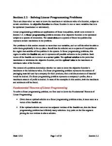
In a message-passing system, the time to send messages must be considered in the overall execution time of a problem. The parallel execution time (tp) is composed of two parts, a computation part (tcomp) and a communication part (tcomm): tp = tcomp + tcomm. Firstly, we shall consider the resolution of the example using parallel dynamic programming with no interpolation (the partition of the set U is not necessary) in two cases: with and without the constraints in the control variables defined in (12). Figures 6 and 7 show the speedup obtained as the number of processors is increased. Constraints reduce the absolute computational burden as they reduce the number of quantized states and controls to consider [3]. However, it is impossible to know in advance what constraints will activate (only active constraints actually reduce the computational load). For this reason, it is not possible to send the same amount of work to each processor: there exists imperfect load balancing between slaves (Figure 8). Even though the parallel execution time is greater without constraints (there is no reduction in the number of controls or states), the speedup is much better, almost linear, as the load balancing is almost perfect (Figure 9). The behaviour of the parallel algorithms with interpolation is similar (Figure 10). After analyzing both implementations (P_DP_I_S and P_DP_I_C), it is shown and proven [20] how parallel processing in the controls presents a smaller parallel execution time than parallel processing in the states.
P_DP with control constraints
14
P_DP without control constraints
13
Lineal speedup
12
S(M), speedup factor
A measure of the relative performance between a multiprocessor system and a single processor system is the speedup factor, S(M) = ts / tp, where ts is the execution time using one processor and tp is the execution time using a multiprocessor with M processors.
15
11 10 9 8 7 6 5 4 3 2 1 0 1
2
3
4
5
6
7
8
9
10
11
12
13
14
15
Number of processors (M)
Figure 7: Speedup factor (P_DP: parallel dynamic programming with no interpolation), ∆xi = 0.25, i = 1, 2, 3.
7 Conclusions This paper has shown how the great disadvantage of the dynamic programming techniques, its great computational complexity, can be reduced with parallel processing on clusters of PCs. Parallel algorithms have been proposed and it has been shown how constraints, even they reduce the global computational burden, contribute to an imperfect load balancing.
References [1] R. E. Bellman, “Dynamic Programming”, Princeton University Press, New Jersey, 1957.
[2] R. E. Bellman and S. E. Dreyfus, “Applied Dynamic Programming”, Princeton University Press, New Jersey, 1962. [3] A. P. de Madrid, S. Dormido, F. Morilla. “Reduction of the Dimensionality of Dynamic Programming: A Case Study”, American Control Conference ACC99. San Diego, USA, 1999. [4] R. E. Larson, “State Increment Dynamic Programming”, American Elsevier Publishing Company, INC, New York, 1968.
550
P_DP_I_S with control constraints
500
P_DP_I_C with control constraints
450 400
tp (seconds)
350 300 250 200 150 100 50 0 0
Figure 8: Communications with control constraints.
1
2
3
4
5
6
7
8
9
10 11
12 13 14
15
Number of processors (M)
Figure 10: Parallel execution time (P_DP_I_S: parallel dynamic programming with interpolation and paralelization in the states; P_DP_I_C: parallel dynamic programming with interpolation and paralelization in the controls), ∆xi = 0.5, ∆u i = 0.25, i = 1, 2, 3.
[13] R. E. Larson and E. Tse, “Parallel Processing
[14] Figure 9: Communications without control constraints.
[5] S. Dormido, M. Mellado and J. M. Guillen,
[6]
[7]
[8] [9] [10]
[11] [12]
“Consideraciones sobre la regulación de Sistemas Mediante Técnicas de Programación Dinámica”, Revista Automática, 10, pp. 29-34, 1970. R. E. Larson and A. J. Korsak, “A Dynamic Programming Succesive Approximations Technique with Convergence Proofs”, Part I, Automatica, 6, pp. 245-252, 1970. A. J. Korsak and R. E. Larson, “A Dynamic Programming Succesive Approximations Technique with Convergence Proofs”, Part II, Automatica, 6, pp. 253-260, 1970. L. Cooper and M. W. COOPER, “Introduction to Dynamic Programming”, Pergamon Press, 1981. R. E. Larson and J. L. Casti, “Principles of Dynamic Programming. Part II: Advanced Theory and Applications”, Marcel Dekker, Inc., New York, 1982. L. Moreno, L. Acosta and J. L. Sánchez, “Design of Algorithms for Spacial-time Reduction Complexity of Dynamic Programming”, IEE Proc.-D, 139, 2, pp. 172-180, 1992. M. Sniedovich, “Dynamic Programming”, Marcel Dekker, Inc., New York, 1992. A. P. de Madrid, S. Dormido, F. Morilla and L. Grau, “Dynamic Programming Predictive Control”. IFAC, 13th Triennial World Congress, 2c-02, pp. 279-284, San Francisco, USA, 1996.
[15]
[16] [17] [18] [19]
[20]
[21]
Algorithms for the Optimal Control of Nonlinear Dynamic Systems”, IEEE Transactions on Computers, C-22, 8, pp. 777-786, 1973. A. Geist, A. Beguelin, J. Dongarra, W. Jiang, R. Mancher and V. Sunderam, “PVM: Parallel Virtual Machine. A Users’ Guide and Tutorial for Networked Parallel Computing”, The MIT Press, Cambridge, Massachussetts, 1994. R. E. Larson and J. L. Casti, “Principles of Dynamic Programming. Part I: Basic Analytic and Computational Methods”, Marcel Dekker, Inc., New York, 1978. D. A. Pierre, “Optimization Theory with Applications”, Dover Publications, Inc., New York, 1986. E. Mosca, “Optimal, Predictive and Adaptive Control”, Prentice Hall, New Jersey, 1995. J. J. G. Guignabodet, “Analysis of some Process Aspects of Dynamic Programming”, Ph.D. Thesis, Washington University, 1961. J. F. Baldomero, “PVMTB: Parallel Virtual Machine ToolBox”, II Congreso de Usuarios Matlab’99, Dpto. Informática y Automática, UNED, pp. 523532, Madrid, 1999. S. D. Canto, “Programación Dinámica Paralela: Aplicación a Problemas de Control”, Ph.D. Thesis, Dpto. Informática y Automática (UNED), Madrid, 2002. B. Wilkinson and M. Allen, “Parallel Programming: Techniques and Applications Using Networked Workstations and Parallel Computers”, Prentice Hall, 1999.