N. de Freitas, âSample efficient actor-critic with experience replay,â in. International Conference on Learning Representations (ICLR), 2017. [26] S. Gu, T. Lillicrap ...
Deep Dynamic Policy Programming for Robot Control with Raw Images Yoshihisa Tsurumine1 , Yunduan Cui1 , Eiji Uchibe2 and Takamitsu Matsubara1
Abstract— Deep reinforcement learning has drawn much attention in robot control since it enables agents to learn control policies from very high dimensional states such as raw images. On the other hand, its dependency upon the availability of a significant quantity of training samples and its fragility in learning makes it difficult to apply for real world robot tasks. To alleviate these issues we propose Deep Dynamic Policy Programming (DDPP), which combines the sample efficiency and smooth policy updates of dynamic policy programming with the contemporary deep reinforcement learning framework. The effectiveness of the proposed method is first demonstrated in a simulation of the robot arm control problem, with comparison to Deep Q-Networks. As validation on a real robot system, DDPP also successfully learned the flipping of a handkerchief with a NEXTAGE humanoid robot using a reduced number of learning samples, whereas Deep Q-Networks failed to learn the task.
I. I NTRODUCTION With the capability of searching for optimal policies by interacting with their environments without any prior knowledge, Reinforcement Learning (RL) [1] has been successfully applied to a broad range of robot control tasks. However, its application towards real-world robots still suffers from the intractable computational complexity of high-dimensional state spaces (usually raw data from devices such as cameras), and the learning divergence caused by insufficient samples from real-world systems due to the significant effort required for accumulating adequate data; respectively the curses of dimensionality and issue of limited samples [2, 3]. Owing to recent advances in Deep Learning (DL), improved extraction of high-level features from raw sensory data rather than the traditional usage of handcrafted features has become possible for computer vision [4]–[6] and speech recognition [7, 8] problems. On the other hand, the direct application of DL to robot control is challenging primarily due to the difficulties in accumulating the requisite amounts of training data. A significant progress has been made by combining DL with RL, resulting in the Deep Q-Network (DQN) [9]. By approximating the value function by a deep neural network, the resultant control policy achieved humanlevel performance on various Atari video games given raw images as input. The DL part in DQN provides a good solution to the curse of dimensionality in RL by automatically abstracting good high level features from raw and high dimensional data. Although several extensions of DQN [10, 11] have since been documented with better learning 1 Y. Tsurumine, Y. Cui and T. Matsubara are with the Graduate School of Information Science, Nara Institute of Science and Technology (NAIST), Nara, Japan 2 E. Uchibe is with the Advanced Telecommunications Research Institute International (ATR), Kyoto, Japan.
Fig. 1: The NEXTAGE humanoid robot flipping a handkerchief.
performance in simulations and video games, the application of DQN-like algorithms to real robot control remains limited because the generation of sufficient training samples is still too arduous for physical robot systems. The motivation of this research is to develop DQN-like algorithms with fast convergence and sample efficiency that are applicable to real-world robot tasks. As a RL algorithm that stabilizes the learning of the value function with a limited number of samples, Dynamic Policy Programming (DPP) [12, 13] exploits the nature of the smooth policy update by considering the Kullback-Leibler divergence between current and new policies as a regularization term. In this work Deep Dynamic Policy Programming (DDPP) is proposed, which abstracts features from high-dimensional raw sensory data, approximates its value function by DL with both common and duel network architectures [11], and inherits DPP’s sample usage efficiency. After investigating the scalability of DDPP by comparing it with DQN and duel DQN in a simulated n DOF manipulator reaching task (n = 6, 15), we apply DDPP to control a NEXTAGE humanoid robot to learn the flipping of a handkerchief (shown in Fig. 1) with a limited number of samples as a real-world validation exercise. The remainder of this paper is organized as follows. The introduction of RL and DPP are presented in Section II-A and II-B, we detail DDPP and its duel network structure in Section II-C and II-D. Section III presents the simulation results, with the results of real robot experimentation presented in Section IV. Conclusions and discussions follow in Section V.
II. A PPROACH A. Reinforcement Learning RL [1, 2] usually solves a Markov decision process (MDP) defined by the 5-tuple (S, A, T , R, γ). S = {s1, s2, ..., s n } is a finite set of states. A = {a1, a2, ..., a m } is a finite set of actions. Tssa0 is the probability of transitioning from state s to state s 0 under action a. When transitioning from state s to a from state s 0 under the action a, the agent gets the reward r ss 0 reward function R. γ ∈ (0, 1) is the discount parameter. The policy π(a| s) represents the probability of action a being taken under state s. The value function is defined as the expected discounted total reward in state s: Vπ (s) = Eπ, T where r s t =
P
a ∈A s 0 ∈S
∞ �X
� γ t r s t s0 = s t=0
(1)
π(a| st )Ts tas0 r sat s0 is the expected reward
from state st . The aim of RL is to find an optimal policy π ∗ that maximizes the value function that satisfies the following Bellman equation: X a 0 � Vπ (s) = π(a| s)Tssa0 r ss 0 + γVπ (s ) , (2) a ∈A s 0 ∈S
0
s 0 ∈S
exp ηVπ¯t+1 (s)
�
.
(6)
The action preferences function [1] at the (t + 1)-iteration for all state-action pairs (s, a) is defined following [13] to obtain the optimal policy that maximizes the value function above: X 1 a t 0 � Tssa0 r ss Pt+1 (s, a) = log π¯ t (a| s) + 0 + γVπ ¯ (s ) . (7) η 0 s ∈S
Combining Eq. (7) with Eqs. (5) and (6), a simple form is obtained: X � 1 Vπ¯t (s) = log exp ηPt (s, a) (8) η a ∈A � exp ηPt (s, a) π¯ (a| s) = P �. 0 a 0 ∈A exp ηPt (s, a ) t
(9)
The TD error of action preference function, Pt+1 (s, a) = OPt (s, a), is calculated by plugging Eqs. (8) and (9) into Eq. (7): X a 0 � Tssa0 r ss Pt (s, a) − Lη Pt (s) + 0 + γL η Pt (s ) (10) s 0 ∈S
or a Q function for state-action pairs (s, a): X X 0 0 0 0 � a Q π (s, a) = Tssa0 r ss π(a | s )Q π (s , a ) . 0 +γ s ∈S
π¯ t+1 (a| s) =
f P g a + γV t (s 0 ) � π¯ t (a| s) exp η Tssa0 r ss 0 π¯
0
(3)
a ∈A
The value based RL algorithms, e.g., Q-learning [14], SARSA [15] and LSPI [16], attempt to approximate the value (or Q) function according to the Temporal Difference (TD) error of samples in model free without knowledge of the state transition models and reward function. In Q-learning, the TD update rule follows Q(st , at ) ← Q(st , at )+α[r satts t +1 + γ maxa t +1 Q(st+1, at+1 ) − Q(st , at )] with learning rate α. B. Dynamic Policy Programming
where Lη P(s) , η1 log a ∈A exp(ηP(s, a)) = Vπ¯ (s). The original DPP is only applicable to problems with discrete states and prior knowledge about the underlying model. Sampling-based Approximate Dynamic Policy Programming (SADPP) [12] extends it to model-free learning with continuous states. For N training samples, [s n, a n ]n=1:N , SADPP approximates P(s, a) via Linear Function Approximation ˆ n, a n ; θ) = φ(x n ) T θ where φ(x n ) denotes the (LFA): P(s output vector of basis functions, and θ is the corresponding weight vector. The weight vector is updated by minimizing ˆ , kΦθ − O Pk ˆ 2 where the empirical loss function J(θ; P) 2 ˆ ˆ O P is N × 1 matrix with elements O P(s, a; θ) following Eq. (10) where Lη P(s) is translated into a Boltzmann softmax operator for more analytically tractable recursion. DPP has been applied to real robot control problems [18, 19] with sample efficiency. However, due to the exponentially growing size of basis functions with increasing input dimensionality and the corresponding intractability it brings, the application of DPP to raw data such as images remains prohibitive. P
In order to exploit the nature of the smooth policy update, DPP [12, 13] considers the Kullback-Leibler divergence between the current policy π and the baseline policy π¯ in its value function, to minimize the difference between the current and baseline policy while maximizing the expected reward: � X � π(a| s)�� C. Deep Dynamic Policy Programming a ∗ 0� 1 log . (s ) − Vπ¯∗ (s) =max π(a| s) Tssa0 r ss 0+γVπ ¯ (4) π η π(a| ¯ s) Following DQN’s approximation of the Q function by a ∈A s 0 ∈S Convolutional Neural Networks (CNNs), we propose DDPP ˆ a; θ) The balance of the Kullback-Leibler divergence is controlled to approximate the action preferences function P(s, by deep neural networks with parameter θ in this section. by inverse temperature η. Following [12, 17], we let η be a ∗ DDPP’s network structure is defined following Fig. 2. The positive constant. The optimal value function Vπ¯ (s) for all ∗ initial input state s is raw image (with RGB or grayscale) that s ∈ S, and the optimal policy π¯ (a| s) for all (s, a), both usually has very high dimensionality. Preprocessing the raw satisfy a double-loop with fixed point iterations: image by a CNN abstracts the image to a lower-dimensional f X g 1 X a t 0 � high-level feature set. These features are in turn processed Vπ¯t+1 (s) = log π¯ t(a| s)exp η Tssa0 r ss 0 +γVπ (5) ¯ (s ) η a ∈A by Fully Connected Networks (FCNs), the final layer having 0 s ∈S
Raw Image Data
Abstracted Features
Convolutional Neural Networks
Fully Connected Networks
Fig. 2: Network architectures of Deep Dynamic Policy Programming.
m nodes, where m is the number of actions in A, the i-th ˆ ai ; θ). node’s output being the approximated value P(s, According to [9], DQN defines a target network as Q(s, ˆa, θ − ) to stabilize learning. While θ − is updated every C steps by θ − = θ, DQN’s parameters θ are updated every a step with sample (s j , a j , r s jjs j+1 , s j+1 ) from a global memory storing all generated samples by performing a gradient descent step on the TD error: a
ˆ j+1, a 0; θ − )− Q(s ˆ j , a j ; θ)) 2 . (11) J(θ; Qˆ ) , (r s jjs j+1+γ max Q(s a0 Without avoiding excessively large policy update via Kullback- Leibler divergence, the gradient descent step above may be too large to smoothly update θ − , therefore slows down the learning and cripples sample efficiency. On the other hand, thanks to the nature of smooth policy update, DDPP is capable to have a more efficient learning with stability following Algorithm 1 Compared with DQN, it achieves: 1) a local memory D with the current E iteration’s samples is applied to store less samples and focuses more on new samples. 2) update θ every episode with T steps rather than every step. 3) the update in each episode is divided to N sub problems that continuously update θ until reaching a given threshold. In DDPP, each iteration i has M episodes with a total M × T samples. A local memory D is maintained to store the current E iterations’ samples for experience feedback. The updating of networks is operated every episode. The current parameters as θ − is saved to build target network ˆ a; θ − ). The update is divided into N sub problems. P(s, In each one, the agent repeatedly collects mini-batches of a samples (s j , a j , r s jjs j+1 , s j+1 ) is from D and calculates the teaching signal y j following Eq. (10):
Algorithm 1: Deep Dynamic Policy Programming Initialize local memory D and its size E Initialize network weights θ Initialize target network weights θ − = θ Initialize threshold, ratio for i = 1, 2, ..., I do for episode = 1, 2, ..., M do for t = 1, 2, ..., T do Take action at with softmax policy based on ˆ t , at ; θ) and Eq. (9) π¯ t (at | st ) following P(s Receive new state st+1 and reward r satts t +1 Store transition (st , at , r satts t +1 , st+1 ) in D for n = 1, 2, ..., N do Set average = 0 repeat Sample random minibatch of transition a (s j , a j , r s jjs j+1 , s j+1 ) in D Calculate the teaching signal: ˆ j , a j ; θ − )−Lη P(s ˆ j ; θ − )+r sa js + y j = P(s j j+1 − ˆ j+1 ; θ ) γLη P(s Get loss and update θ by performing a ˆ j , a j ; θ)) 2 gradient descent step on (y j − P(s average = ratio × average + (1 − ratio) × loss until average < threshold; Update the target network θ − = θ if i > (E − 1) then Update D to store the current (E − 1) iterations’ samples
The loss of gradient descent’s is added to the average loss. When the average loss is less than a threshold, the current sub-update is terminated and the target networks are updated after processing N minibatch by θ − = θ. The N time sub-updating efficiently utilizes samples to accelerate training. By limiting overly large updates, it reduces the average loss between current and target networks to a threshold while avoiding divergence. D. Duel DDPP
The Duel DQN has a new neural network architecture with two parts to automatically produces separate estimates of the value function V (s) and advantage function A(s, a) that fulfills A(s, a) = Q(s, a) − V (s), without any extra supervision. It leads to dramatic improvements over existing approaches for deep RL according to [11]. However, to our best knowledge, Duel DQN was mainly applied to Atari games with tediously long training, which would limit application to real-world robot control due to the same reason for DQN. aj We propose how DDPP can be naturally extended to a − − − ˆ ˆ ˆ y j = P(s j , a j ; θ )−Lη P(s j ; θ )+r s j s j+1+γLη P(s j+1 ; θ ). (12) duel network (Fig. 3) in this subsection. Plugging Lη P(s) , P 1 The networks parameters are updated by running gradient η log a ∈A exp(ηP(s, a)) = Vπ¯ (s) into Eq. (10), we obtain: X descent algorithms to minimize the loss function: � a t Pt+1 (s, a) = Pt (s, a) − Vπ¯t (s) + Tssa0 r ss 0 + γVπ ¯ (s) . (14) 2 ˆ , (y j − P(s ˆ j , a j ; θ)) . (13) J(θ; P) s 0 ∈S
Raw Image Data
Abstracted Features
Convolutional Neural Networks
Fully Connected Networks
Fig. 3: Network architectures of Duel Deep Dynamic Policy Programming. Fig. 5: Learning curves for 6 DOF manipulator reaching task.
Fig. 4: The input image of N = 6 DOF manipulator reaching task in simulation, different colors represent the manipulator in different steps.
Combine Eq. (14) with Eq. (7), the action preference function can be represented as: Pt (s, a) =
1 log π¯ t (a| s) + Vπ¯t (s). η
(15)
It naturally divides the action preference function into two parts: η1 log π¯ t (a| s) that can be treated as advantage function A(s, a) and Vπ¯t (s) is the value function. Figure 3 shows the network architecture of Duel DDPP that consists of two streams that represent the value and advantage functions respectively while sharing a same convolutional feature abstraction module. III. S IMULATION R ESULT In this section, the learning performance of DDPP and Duel DDPP is investigated in a simulated n DOF manipulator reaching task (n = 6, 15) with comparison of DQN and Duel DQN. The state is the entirety of a grayscale 84 × 84 px image where the n DOF manipulator is drawn following Fig. 4. Each joint has five discrete actions [−0.0875, −0.0175, 0, 0.0175, 0.0875] (rad) to increment the joint with the respective angle. We define an action at each time step as one move per joint so the total number of actions is reduced to (n × 5). The first joint is set to position [0, 0]. The length of each limb between two joints is set to 1 n m. All angles are initialized to 0 rad at the start of the simulation. The target position to reach in two dimensional
Fig. 6: Learning curves for 15 DOF manipulator reaching task.
axes is set as Xtarget = 0.6830, Ytarget = 0, and the reward � function is set as r = − |Xtarget − X | + |Ytarget − Y | where X, Y is the current position of the manipulator’s end-effector. Each iteration operates M = 5 episodes with T = 30 steps. The local memory is set for E = 3 iteration. The policy of DDPP and Duel DDPP is calculated by Eq. (9) while DQNs use an ε-greedy policy. All the results are derived from five repetitions of the same experiment. We used a computer with Intel Core i7-5960 CPU, Nvidia GTX 1080 GPU and 64 GB memory. The experimental platform is built in Tensorflow [20] and Keras [21]. For the network architecture of DDPP and DQN, the input layer has 84×84×1 nodes for each pixel of the state image. It is processed by a three layered CNN: the first layer convolves 32 8 × 8 filters with stride 4, the second convolves 64 4 × 4 filters with stride 2 and the third convolves 64 3 × 3 filters with stride 1. The final hidden layer is a FCN consisting of 512 rectifier units. The activation function of both CNNs and FCN employs ReLU (Rectified Linear Unit). For the Duel
Observe State from raw image data
Take action & get reward
6 points for picking up
Fig. 8: Four selected features of 1st CNN layer learned by Duel DDPP in real robot experiment, the color of grid indicates the weight of RGB in the current filter. 6 points for dropping down
Reward = ratio of red area over the whole image
Fig. 7: The experimental setting of NEXTAGE robot on the task of flipping a handkerchief.
DDPP and DQN, FCN is divided by two parts: 256 units for approximating the value function V (s), and 256 units for η1 log π¯ (a| s). RMSprop is used as the gradient descent method to update the neural networks’ parameters. According to Figs. 5 and 6, both DDPP and Duel DDPP performed well as expected in simulations: they stably improved their performance with only around 2000 samples (14 iterations) while DQN and Duel DQN could not. Moreover, by separately learning the action preference function, Duel DDPP outperformed DDPP in all simulations. These results indicate DDPP’s sample efficiency and show its potential to be applied in real-world robot control. IV. R EAL ROBOT E XPERIMENT In this section, Duel DDPP is applied to control the NEXTAGE robot (www.nextage.kawada.jp/en/), a 15 DOF humanoid robot with sufficient precision for manufacturing tasks, to learn the flipping of a handkerchief from its green side over to its red side. As shown in Fig. 7, the input state is a 84 × 84 px RGB image from the NEXTAGE’s integrated camera. 6 × 6 = 36 grippers’ actions are defined as picking up the handkerchief from a 2 × 3 points over the current handkerchief’s area and dropping it down to 2×3 points over the table. The reward is r = 5 × Ar ed where Ar ed is the ratio of the red area over the whole image in the current state. In each episode, the handkerchief is initially placed green side up by a human, and processed by the NEXTAGE with 30 actions. All parameters are updated every five episodes, i.e., one iteration. Both the network architecture and computing setup are identical to that in Section II-D, whereas now the input layer has 84 × 84 × 3 nodes for each pixel of the state image. To optimize the learning results, both Duel DPP and Duel DQN’s parameters are manually tuned. According to the learning results shown in Fig. 9, Duel DDPP outperformed Duel DQN by total reward with only 2400 samples (= 16 iterations). The whole training period took approx. four hours including 40 minutes for manually
initializing the handkerchief (≈ 30 seconds per episode). The best states (i.e., the best result over some samples) indicate that the NEXTAGE robot improves its flipping skill during the training using Duel DDPP. It took meaningful actions according to meaningful features abstracted by CNNs (Fig. 8), learned from a limited number of samples clearly displaying the green and red areas. V. C ONCLUSIONS AND D ISCUSSIONS The contribution of this paper is twofold. Algorithmically we propose a new deep reinforcement learning algorithm, DDPP to achieve better sample efficiency by combing smooth policy updates with DQN since the learning of deep networks with limited number of samples is stabilized by the Kullback-Leibler divergence between the current and baseline policies. For novel robot control, DDPP was successfully applied to a NEXTAGE humanoid robot to learn the flipping of a handkerchief from raw image data without a tediously long training period. Another work having a close concept to ours is the Policy Gradient and Q-learning (PGQ) [22] that augments deep reinforcement learning with an entropy regularized policy gradient, which outperformed DQN and Asynchronous Advantage Actor-critic (A3C) [23] in some Atari games. Compared with PGQ, DDPP adds an entropy regularization term in its value function and results in the action preference function P to naturally replace the Q-function. Moreover, its aim is to be applicable to real robot control that requires sample efficiency while PGQ is designed for training over a significantly longer baseline. The extension of current works can be divided into two parts. The first is to design challenging tasks to utilize the feature abstraction of DL further, e.g., driving the robot to handle complex deformable objects such as clothing. Another is extending DDPP, with emphasis on Duel DDPP, to a continuous action domain based on [24]–[26] where the nature of smooth policy update is expected to improve learning performance. VI. ACKNOWLEDGMENT We gratefully acknowledge the support from the New Energy and Industrial Technology Development Organization (NEDO) for this research. We also thank Mr. James Poon for proofreading.
Fig. 9: The experimental results of NEXTAGE humanoids robot on the task of flipping a handkerchief over three repetitions. The left side is the average learning line of the total reward with exponential smoothing and the baseline of random actions. The right side is Duel DDPP’s best state over the 600, 1200, 1800, 2400 samples during learning.
R EFERENCES [1] R. S. Sutton and A. G. Barto, Reinforcement learning: An introduction. MIT press Cambridge, 1998. [2] J. Kober, J. A. Bagnell, and J. Peters, “Reinforcement learning in robotics: A survey,” The International Journal of Robotics Research, vol. 32, no. 11, pp. 1238–1274, 2013. [3] S. Schaal and C. G. Atkeson, “Learning control in robotics,” IEEE Robotics & Automation Magazine, vol. 17, no. 2, pp. 20–29, 2010. [4] A. Krizhevsky, I. Sutskever, and G. E. Hinton, “Imagenet classification with deep convolutional neural networks,” in Advances in neural information processing systems (NIPS), pp. 1097–1105, 2012. [5] V. Mnih, Machine learning for aerial image labeling. PhD thesis, University of Toronto, 2013. [6] C. Szegedy, W. Liu, Y. Jia, P. Sermanet, S. Reed, D. Anguelov, D. Erhan, V. Vanhoucke, and A. Rabinovich, “Going deeper with convolutions,” in IEEE Conference on Computer Vision and Pattern Recognition (CVPR), pp. 1–9, 2015. [7] G. E. Dahl, D. Yu, L. Deng, and A. Acero, “Context-dependent pretrained deep neural networks for large-vocabulary speech recognition,” IEEE Transactions on Audio, Speech, and Language Processing, vol. 20, no. 1, pp. 30–42, 2012. [8] A. Graves, A.-r. Mohamed, and G. Hinton, “Speech recognition with deep recurrent neural networks,” in IEEE international conference on acoustics, speech and signal processing (ICASSP), pp. 6645–6649, 2013. [9] V. Mnih, K. Kavukcuoglu, D. Silver, A. A. Rusu, J. Veness, M. G. Bellemare, A. Graves, M. Riedmiller, A. K. Fidjeland, G. Ostrovski, et al., “Human-level control through deep reinforcement learning,” Nature, vol. 518, no. 7540, pp. 529–533, 2015. [10] H. Van Hasselt, A. Guez, and D. Silver, “Deep reinforcement learning with double Q-learning.,” in Association for the Advancement of Artificial Intelligence (AAAI), pp. 2094–2100, 2016. [11] Z. Wang, T. Schaul, M. Hessel, H. Van Hasselt, M. Lanctot, and N. De Freitas, “Dueling network architectures for deep reinforcement learning,” in International Conference on Machine Learning (ICML), ICML’16, pp. 1995–2003, 2016. [12] M. G. Azar, V. Gómez, and H. J. Kappen, “Dynamic policy programming with function approximation,” in International Conference on Artificial Intelligence and Statistics (AISTATS), pp. 119–127, 2011. [13] M. G. Azar, V. Gómez, and H. J. Kappen, “Dynamic policy programming,” The Journal of Machine Learning Research, vol. 13, no. 1, pp. 3207–3245, 2012.
[14] C. J. Watkins and P. Dayan, “Q-learning,” Machine learning, vol. 8, no. 3-4, pp. 279–292, 1992. [15] R. S. Sutton, “Generalization in reinforcement learning: Successful examples using sparse coarse coding,” Advances in neural information processing systems (NIPS), pp. 1038–1044, 1996. [16] M. G. Lagoudakis and R. Parr, “Least-squares policy iteration,” The Journal of Machine Learning Research, vol. 4, no. 44, pp. 1107–1149, 2003. [17] E. Todorov, “Linearly-solvable markov decision problems,” in Advances in neural information processing systems (NIPS), pp. 1369– 1376, 2006. [18] Y. Cui, T. Matsubara, and K. Sugimoto, “Pneumatic artificial muscledriven robot control using local update reinforcement learning,” Advanced Robotics, pp. 1–16, 2017. [19] Y. Cui, T. Matsubara, and K. Sugimoto, “Kernel dynamic policy programming: Practical reinforcement learning for high-dimensional robots,” in IEEE-RAS International Conference on Humanoid Robots (Humanoids), pp. 662–667, 2016. [20] M. Abadi, A. Agarwal, P. Barham, E. Brevdo, Z. Chen, C. Citro, G. S. Corrado, A. Davis, J. Dean, M. Devin, et al., “Tensorflow: Largescale machine learning on heterogeneous distributed systems,” arXiv preprint arXiv:1603.04467, 2016. [21] F. Chollet et al., “Keras.” https://github.com/fchollet/ keras, 2015. [22] B. O’Donoghue, R. Munos, K. Kavukcuoglu, and V. Mnih, “PGQ: Combining policy gradient and Q-learning,” arXiv preprint arXiv:1611.01626, 2016. [23] V. Mnih, A. P. Badia, M. Mirza, A. Graves, T. P. Lillicrap, T. Harley, D. Silver, and K. Kavukcuoglu, “Asynchronous methods for deep reinforcement learning,” in International Conference on Machine Learning (ICML), pp. 1928–1937, 2016. [24] T. P. Lillicrap, J. J. Hunt, A. Pritzel, N. Heess, T. Erez, Y. Tassa, D. Silver, and D. Wierstra, “Continuous control with deep reinforcement learning,” arXiv preprint arXiv:1509.02971, 2015. [25] Z. Wang, V. Bapst, N. Heess, V. Mnih, R. Munos, K. Kavukcuoglu, and N. de Freitas, “Sample efficient actor-critic with experience replay,” in International Conference on Learning Representations (ICLR), 2017. [26] S. Gu, T. Lillicrap, Z. Ghahramani, R. E. Turner, and S. Levine, “Qprop: Sample-efficient policy gradient with an off-policy critic,” in International Conference on Learning Representations (ICLR), 2017.