Dynamic, Real-time Forecasting of Online Auctions via Functional Models Wolfgang Jank
Galit Shmueli
Shanshan Wang
Department of Decision and Information Technologies Robert H. Smith School of Business University of Maryland
Department of Decision and Information Technologies Robert H. Smith School of Business University of Maryland
Statistics Program Department of Mathematics University of Maryland
[email protected]
[email protected]
[email protected]
ABSTRACT
which of these numerous auctions to participate and to place a bid. The decision making process of an eBay bidder can be supported by information on price forecasts. If one had a method to predict the outcome of an auction ahead of time, then one could use these predictions to create an auctionranking (from lowest predicted price to highest) and select those auctions with the lowest predicted price. One of the difficulties with such an approach is that information in the online environment changes at every moment: new auctions enter the market, old (i.e. closed) auctions drop out, and even within the same auction the price changes constantly with every new incoming bid. Thus, a well-functioning forecasting system has to be adaptive to accommodate ever occurring change. We propose a dynamic forecasting model that can adapt to change. In general, price forecasts can be done in two different ways, in a static and in a dynamic way. The static model relates information that is known before the start of the auction to information that becomes available after the auction closes. This is the basic principle of some of the existing proposed models [Ghani and Simmons, 2004, Ghani, 2005, Lucking-Reiley et al., 2000, Bajari and Hortacsu, 2003]. For instance, one could relate the opening bid, the auction length and a seller’s reputation to the final price. Notice that opening bid, auction length, and seller reputation are all known at the auction start. Training a model on a suitable set of past auctions, one can get static forecasts of the final price in that fashion. However, this approach does not take into account important information that arrives during the auction. The number of competing bidders right now or the current price level are factors that are only revealed during the ongoing auction and that are important in determining the future price. Moreover, the current change in price could also have a huge impact on the future price. If, for instance, the price had increased at an extremely fast rate over the last several hours, causing bidders to drop out of the bidding process or to revise their bidding strategies, then this could have an immense impact on the evolution of price in the next few hours and, subsequently, on the final price. We refer to models that account for newly arriving information and for the rate at which this information changes as dynamic models. Forecasting price in online auctions dynamically is challenging for a variety of reasons. Traditional methods for
We propose a dynamic model for forecasting price in online auctions. One of the key features of our model is that it operates during the live-auction, which makes it different from previous approaches that only consider static models. Our model is also different with respect to how information about price is incorporated. While one part of the model is based on the more traditional notion of an auction’s pricelevel, another part incorporates its dynamics in the form of a price’s velocity and acceleration. In that sense, it incorporates key features of a dynamic environment such as an online auction. The use of novel functional data methodology allows us to measure, and subsequently include, dynamic price characteristics. We illustrate our model on a diverse set of eBay auctions across many different book categories. We find significantly higher prediction accuracy compared to standard approaches.
1. INTRODUCTION eBay (www.eBay.com) is the the world’s largest Consumerto-Consumer (C2C) online auction house. In 2005, eBay had about 135 million registered users. There are approximately 44 million items available worldwide on eBay at any given time and approximately 4 million new items are added every day in over 50,000 categories. On eBay.com, an identical (or near-identical) product is often sold in numerous, often simultaneous auctions. For instance, a simple search under the key words “iPod shuffle 512MB MP3 player” returns over 300 hits for auctions that close within the next 7 days. A more general search under the less restrictive key words “iPod MP3 player” returns over 3,000 hits. Clearly, it would be challenging, even for a very dedicated eBay user, to inspect and simultaneously monitor all of these 300 (or 3,000) auctions, while being on the look-out for newly added auctions for the same product, and subsequently deciding in
Permission to make digital or hard copies of all or part of this work for personal or classroom use is granted without fee provided that copies are not made or distributed for profit or commercial advantage and that copies bear this notice and the full citation on the first page. To copy otherwise, to republish, to post on servers or to redistribute to lists, requires prior specific permission and/or a fee. KDD’06, August 20–23, 2006, Philadelphia, Pennsylvania, USA. Copyright 2006 ACM 1-59593-339-5/06/0008 ...$5.00.
1
2.1
forecasting time-series, such as exponential smoothing or moving averages, cannot be applied in the auction context, at least not directly, due to the special data structure. Traditional forecasting methods assume that data arrive in evenlyspaced time intervals such as every quarter or every month. In such a setting, one trains the model on data up to the current time period t, and then uses this model to predict at time t + 1. Implied in this process is the important assumption that the distance between two adjacent time periods is the same, which is the case for quarterly or monthly data. Now consider the case of online auctions. Bids arrive in very unevenly-spaced time intervals, determined by the bidders and their bidding strategies, and the number of bids within a short period of time can sometimes be very sparse, othertimes extremely dense. In this setting, the distance between t and t+1 can sometimes be more than a day, while at other times it may only be a few seconds. Traditional forecasting methods also assume that the time-series continues, at least in theory, for an infinite amount of time and does not stop at a point in the near future. This is clearly not the case in a 5- or 7-day online auction. The implication of this is a discrepancy in the estimated forecasting uncertainty. And lastly, online auctions, even for the same product, can experience price paths with very heterogeneous price dynamics [Jank and Shmueli, 2005, Shmueli and Jank, 2006]. By price dynamics we mean the speed at which price travels during the auction and the rate at which this speed changes. Traditional models do not account for instantaneous change and its effect on the price forecast. This calls for new methods that can measure and incorporate this important information. In this work we propose a new approach for forecasting price in online auctions. The approach allows for dynamic forecasts in that it incorporates information from the ongoing auction. It overcomes the unevenly spacing of data, and also incorporates change in the price dynamics. Our forecasting approach is housed within the principles of functional data analysis [Ramsay and Silverman, 2005]. In Section 2 we explain the principles of functional data analysis and derive our functional forecasting model in Section 3. We apply our model to a set of bidding data for a variety of book auctions in Section 4. We conclude with further remarks in Section 5.
The Price Curve and its Dynamics
A functional data set consists of a collection of continuous functional objects such as the price increases in an online auction. Despite their continuous nature, limitations in human perception and measurement capabilities allow us to observe these curves only at discrete time points. Thus, the first step in a typical functional data analysis is to recover, from the observed data, the underlying continuous functional object [Ramsay and Silverman, 2005]. This is usually done with the help of smoothers. A variety of different smoothers exist. One very flexible and computational efficient choice is the penalized smoothing spline [Ruppert et al., 2003]. Let τ1 , . . . , τL be a set of knots. Then, a polynomial spline of order p is given by f (t) = β0 + β1 t + · · · + βp tp +
L X
βpl (t − τl )p+ ,
(1)
l=1
where u+ = uI[u≥0] denotes the positive part of the function u. Define the roughness penalty Z PENm (t) = {Dm f (t)}2 dt, (2) where Dm f , m = 1, 2, 3, . . . , denotes the mth derivative of the function f . The penalized smoothing spline f minimizes the penalized squared error Z PENSSλ,m = {y(t) − f (t)}2 dt + λPENm (t), (3) where y(t) denotes the observed data at time t and the smoothing parameter λ controls the trade-off between datafit and smoothness of the function f . Using m = 2 in (3) leads to the commonly encountered cubic smoothing spline. Other possible smoothers include the use of B-splines or radial basis functions [Ruppert et al., 2003]. The choice of the knots influences the resulting smoothing spline. Our goal is to obtain smoothing splines that represent, as much as possible, the price formation process. To that end, our selection of knots mirrors the distribution of bid arrivals [Shmueli et al., 2005]. We also pick the smoothing parameter λ to balance data-fit and smoothness [Wang et al., 2006]. The process of going from observed data to functional data is now as follows. For a set of n functional objects, let tij denote the time of the jth observation (1 ≤ j ≤ ni ) on the ith object (1 ≤ i ≤ n), and let yij = y(tij ) denote the corresponding measurements. Let fi (t) denote the penalized smoothing spline fitted to the observations yi1 , . . . , yini . Then, functional data analysis is performed on the continuous curves fi (t) rather than on the noisy observations yi1 , . . . , yini . For ease of notation we will suppress the subscript i and write yt = f (t) for the functional object and D(m) yt = f (m) (t) for its mth derivative. Consider Figure 1 for illustration. The circles in the top panel of Figure 1 correspond to a scatterplot of the bids (on log-scale) versus their timing. The continuous curve in the top panel shows a smoothing spline of order m = 4 using a smoothing parameter λ = 50. One of our modeling goals is to capture the dynamics of an auction. While yt describes the magnitude of the current price, it does not reveal the dynamics of how fast the price is changing or moving. Attributes that we typically associate with a moving object are its velocity (or its speed )
2. FUNCTIONAL DATA MODELS The technological advancements in measurement, collection, and storage of data have led to more and more complex data-structures. Examples include measurements of individuals’ behavior over time, digitized 2- or 3-dimensional images of the brain, and recordings of 3- or even 4-dimensional movements of objects travelling through space and time. Such data, although recorded in a discrete fashion, are usually thought of as continuous objects represented by functional relationships. This gives rise to functional data analysis (FDA) where the center of interest is a set of curves, shapes, objects, or, more generally, a set of functional observations. This is in contrast to classical statistics where the interest centers around a set of data vectors. In that sense, functional data are not only different from the datastructure studied in classical statistics, but actually generalize it. Many of these new data-structures call for new statistical methods in order to unveil the information that they carry. 2
relatively small, the price acceleration is only moderate. A more systematic investigation of auction dynamics has been done in other places [Jank and Shmueli, 2005, Shmueli and Jank, 2006].
3.5 3.3
Log−Price
3.7
Current Price
0
1
2
3
4
5
6
3.
7
DYNAMIC FORECASTING MODEL
Price Velocity
B Predicted Price Path 0
1
2
3
4
5
6
7
P r i c e
Day of Auction
0.00 0.04
Price Acceleration
A
$50 -
Observed Price Path
−0.06
Second Derivative of Log−Price
C
$100 -
0.00 0.05 0.10 0.15
First Derivative of Log−Price
Day of Auction
0
1
2
3
4
5
6
7
Day of Auction
$0 1
Figure 1: Current price, price velocity (first derivative) and price acceleration (second derivative) for a selected auction. The first graph shows the actual bids together with the fitted curve.
2
3
4
Day
5
t
6
7
Figure 2: Schematic of the dynamic forecasting model of an ongoing auction. As pointed out earlier, the goal is to develop a dynamic forecasting model. By dynamic we mean a model that operates in the live-auction and forecasts price at a future time point of the ongoing auction. This is in contrast to a static forecasting model which makes prediction only about the final price, and which takes into consideration only information available before the start of the auction. Consider Figure 2 for illustration. Assume that we observe the price path from the start of the auction until time t (solid black line). We now want to forecast the continuation of this price path (broken grey lines, labelled “A”, “B”, and “C”). The difficulty in producing this forecast is the uncertainty about the price dynamics in the future. If the dynamics leveloff, then the price increase slows down and we might see a price path similar to A. If the dynamics remain steady, the price path might look like the one in B. Or, if the dynamics sharply increase, then a path like the one in C could be the consequence. Either way, knowledge of the future price dynamics appears to be a key factor! Our dynamic forecasting model consequently consists of two parts: First, we develop a model for the price dynamics. Then, using estimated dynamics, together with other relevant covariates, we derive an econometric model of the final price and use it to forecast the outcome of an auction.
as well as its acceleration. Notice that we can compute the price velocity and price acceleration via the first and second derivatives, D(1) yt and D(2) yt , respectively. Consider again Figure 1. The middle panel corresponds to the price velocity, D(1) yt . Similarly, the bottom panel shows the price acceleration, D(2) yt . The price velocity has several interesting features. It starts out at a relatively high mark which is due to the starting price that the first bid has to overcome. After the initial high speed, the price increase slows down over the next several days, reaching a value close to zero mid-way through the auction. A close-to-zero price velocity means that the price increase is extremely slow. In fact, there are no bids between the beginning of day 2 and the end of day 4 and the price velocity reflects that. This is in stark contrast to the price increase on the last day where the price velocity picks up pace and the price jumps up! The bottom panel in Figure 1 represents price acceleration. Acceleration is an important indicator of dynamics since a change in velocity is preceded by a change in acceleration. In other words, a positive acceleration today will result in an increase of velocity tomorrow. Conversely, a decrease in velocity must be preceded by a negative acceleration (or deceleration). The bottom panel in Figure 1 shows that the price acceleration is increasing over the entire auction duration. This implies that the auction is constantly experiencing forces that change its price velocity. The price acceleration is flat during the middle of the auction where no bids are placed. With every new bid, the auction experiences new forces. The magnitude of the force depends on the size of the price-increment. Smaller price-increments will result in a smaller force. On the other hand, a large number of small consecutive price-increments will result in a large force. For instance, the last 2 bids in Figure 1 arrive during the final moments of the auction. Since the increments are
3.1
Modeling and Forecasting Dynamics
We pointed out earlier that one of the main characteristics of online auctions is their rapid change in dynamics. Since change in the p + 1st derivative precedes change in the pth derivative (e.g. change in acceleration precedes change in velocity), we make use of derivative information for forecasting. In the following, we develop a model to estimate and forecast an auction’s price dynamics. Let again D(m) yt denote the mth derivative of the price yt at time t. We model the derivative curve as a polynomial 3
in time t with autoregressive (AR) residuals, D(m) yt = a0 + a1 t + · · · + ak tk + αx(t) + ut ,
Table 1: Categories of 768 book auctions. The second column gives the number of auctions per category. The third and fourth column show average and standard deviation of price per category.
(4)
where x(t) is a vector of covariates, α is a corresponding vector of parameters, and ut follows an autoregressive model of order p: ut = φ1 ut−1 + φ2 ut−2 + · · · + φp ut−p + εt , εt ∼ N (0, σ 2 ).
Book Category Antiquarian & Collect. Audiobooks Children’s Books Fiction Books Magazines Nonfiction Books Textbooks & Educ. Other
(5)
We allow (4) to depend on the vector x(t), which results in a very flexible model that can accommodate different dynamics due to differences in the auction format or the product category. We estimate model (4) from the training sample. Estimation is done in two steps: First, we estimate the parameters a1 , . . . , ak and α. Then, using the estimated residuals u ˆt , we estimate the values of φ1 , . . . , φp . Forecasting is also done in two steps. Let 1 ≤ t ≤ T denote the observed time periods and let T + 1, T + 2, T + 3, . . . denote time periods we wish to forecast. We first forecast the next residual via u ˜T +1|T = φ˜1 uT + φ˜2 uT −1 + · · · + φ˜p uT −p+1 .
4.1
(6)
4.2
(7)
In a similar fashion, we can predict the derivative l steps ahead: (8) k
a ˆ0 + a ˆ1 (T + l) + · · · + a ˆk (T + l) + ˆ αx(T + l) + u ˜ T +l|T
3.2 Modeling and Forecasting Price After forecasting the price dynamics, we use these forecasts to predict the auction price over the next time periods up to the auction end. Many factors can affect the price in an auction such as information about the auction format, the product, the bidders and the seller. Let x(t) denote the vector of all such factors. Let d(t) = (D(1) yt , D(2) yt , . . . , D(p) yt ) denote the vector of price dynamics, i.e. the vector of the first p derivatives of y at time t. The price at t can be affected by the price at t − 1 and potentially also by its values at times t − 2, t − 3, etc. Let l(t) = (yt−1 , yt−2 , . . . , yt−q ) denote the vector of the first q lags of yt . We then write the general dynamic forecasting model as follows: yt = βx(t) + γd(t) + δl(t) + ǫ t
(9)
where β, γ and δ denote the parameter vectors and ǫ t ∼ N (0, σ 2 ). We use the estimated model (9) to predict the price at T + l as ˆ ˆ ˆ d(T + l) + δl(T y˜T +l|T = βx(T + l) + γ + l)
StDev $165.82 $22.48 $18.03 $9.34 $9.43 $52.83 $37.46 $80.31
Data
Estimated Model
Our model building investigations suggest that among all price dynamics only velocity f ′ (t) is significant for forecasting price in our data. We thus estimate model D(m) yt in (4) only for m = 1. We do so in the following way. Using a quadratic polynomial (k = 2) in time t and influenceweighted predictor variables for book-category (˜ x1 (t)) and shipping costs (˜ x2 (t)) results in an AR(1) process for the residuals ut (i.e. p = 1 in (5)). The rationale behind using book-category and shipping costs in model (4) is that we would expect the dynamics to depend heavily on these two variables. For instance, the category of antiquarian and collectible books typically contains items that are of rare nature and that appeal to a market not as price sensitive and with a strong interest in obtaining the item. This is also reflected in the large average price and even larger variability for items in this category (Table 1). The result of these market differences may well be a different price evolution and thus a difference in price dynamics. A similar argument applies to the shipping costs. Shipping costs are determined by the seller and act as a “hidden” price premium. Bidders are often deterred by excessively high shipping costs and as a consequence auctions may experience differences in the price dynamics. Table 2 summarizes the estimated coefficients averaged across all auctions from the training set. We can see that both book-category and shipping costs result in significantly different price dynamics. After modeling the price dynamics we estimate the price forecasting model (9). Recall that (9) contains three model components, x(t), d(t) and l(t). Among all reasonable pricelags only the first lag is influential, so we have l(t) = yt−1 . Also, as mentioned earlier, among the different price dynamics we only find the velocity to be important, so d(t) = D(1) yt . The first two rows of Table 3 display the correspond-
a ˆ0 + a ˆ1 (T + 1) + · · · + a ˆk (T + 1)k + ˆ αx(T + 1) + u ˜ T +1|T .
D(m) y˜T +l|T =
Mean $89.90 $18.57 $12.89 $7.90 $11.87 $15.63 $19.62 $36.48
Our data set is diverse and contains 768 eBay book auctions from October 2004. All auctions are 7 days long and span a variety of categories (see Table 1). Prices range from $0.10 to $999 and are, not unexpectedly, highly skewed. Prices also vary significantly across the different book categories. This data set is challenging due to its diversity in products and price. We use 70% of these auctions (or 538 auctions) for training purposes. The remaining 30% (or 230 auctions) are kept in the validation sample.
Using this forecast, we can predict the derivative at the next time point T + 1 via D(m) y˜T +1|T =
Count 84 46 102 162 58 239 36 41
(10)
4. EMPIRICAL RESULTS 4
Table 3: Estimates for the price forecasting model (9). The first column indicates the part of the model design that the predictor is associated with. The third column reports the estimated parameter values and the fourth column reports the associated significance levels. Values are again averaged across the training set.
Table 2: Estimates for the velocity model D(1) yt in (4). The second column reports the estimated parameter values and the third column reports the associated significance levels. Values are averaged across the training set. Predictor Intercept t t2 Book Category x ˜1 (t) Shipping Costs x ˜2 (t) ut
Coeff 0.041 -0.012 0.004 1.418 1.684 1.442
P-Val 0.004 0.055 0.041 0.038 0.036 -
Des d(t) l(t) x(t) x(t) x(t) x(t) x(t) x(t) x(t) x(t) x(t)
ing estimated coefficients. Notice that both l(t) and d(t) are predictor variables derived from price, either from its lag or from its dynamics. We also use 8 non-price related predictor variables x(t) = (x1 (t), x2 (t), x3 (t), x ˜4 (t), x ˜5 (t), x ˜6 (t), x ˜7 (t), x ˜8 (t))T . Specifically, the 8 predictor variables correspond to the average rating of all bidders until time t (which we refer to as the current average bidder rating at time t and denote as x1 (t)), the current number of bids at time t (x2 (t)), and the current winner rating at time t (x3 (t)). These first 3 predictor variables are time-varying. We also consider 5 time-constant predictors: the opening bid (˜ x4 (t)), the seller rating (˜ x5 (t)), the seller’s positive ratings only (˜ x6 (t)), the shipping costs (˜ x7 (t)), and the book category (˜ x8 (t)), where x ˜i (t) again denotes the influence-weighted variables. Table 3 shows the estimated parameter values for the full forecasting model. It is interesting to note that bookcategory and shipping costs have low statistical significance. The reason for this is that their effects have likely already been captured satisfactorily in the model for the price velocity. Also notice that the model is estimated on the log-scale for better model fit. That is, the response yt and all numeric predictors (˜ x1 (t), . . . , x ˜7 (t)) are log-transformed. The implication of this lies in the interpretation of the coefficients. For instance, the value 0.051 implies that for every 1% increase in opening bid, the price increases by about 0.05%, on average.
Predictor Price Velocity D(1) yt Price Lag yt−1 Intercept Cur.Avg.Bid.Rating x1 (t) Cur.Numb.Bids x2 (t) Cur.Win.Rating x3 (t) Opening Bid x ˜4 (t) Seller Rating x ˜5 (t) Pos Seller Rating x ˜6 (t) Shipping Cost x ˜7 (t) Book Category x ˜8 (t)
Coeff 0.592 4.824 5.909 0.414 -0.008 0.197 0.051 -11.534 1.518 0.008 3.950
P-Val 0.049 0.044 0.110 0.012 0.027 0.027 0.031 0.070 0.093 0.215 0.107
absolute percentage error (MAPE), that is ¯ 230 ¯ 1 X ¯¯ (Predicted Pricet,i − True Pricet,i ) ¯¯ MAPEt = ¯, 230 i=1 ¯ True Pricet,i i = 1, . . . , N ; t = 6.1, . . . , 7,
where i denotes the ith auction in the validation data. The solid line in Figure 3 corresponds to MAPE for our dynamic forecasting model. We benchmark the performance of our method against double exponential smoothing. Double exponential smoothing is a popular short term forecasting method which assigns exponentially decreasing weights as the observation become less recent and also takes into account a possible (changing) trend in the data. The dashed line in Figure 3 corresponds to MAPE for double exponential smoothing. We notice that for both approaches, MAPE increases as we predict further into the future. However, while for our dynamic model MAPE increases to only about 5% at the auction-end, exponential smoothing incurs an error of over 40%. This difference in performance is relatively surprising, especially given that exponential smoothing is a wellestablished (and powerful) tool in time series analysis. One of the reasons for this underperformance is the rapid change in price dynamics, especially at the auction-end. Exponential smoothing, despite the ability to accommodate for changing trends in the data, cannot account for the price dynamics. This is in contrast to our dynamics forecasting model which explicitly models price velocity. As pointed out earlier, a change in a function’s velocity precedes a change in the function itself, so it seems only natural that modeling the dynamics makes a difference for forecasting the final price.
4.3 Forecasting Accuracy We estimate the forecasting model on the training data and use the validation data to investigate its forecasting accuracy. To that end we assume that for the 230 auctions in the validation data we only observe the price until day 6 and we want to forecast the remainder of the auction. We forecast price over the last day in small increments of 0.1. That is, from day 6 we forecast day 6.1, or the price after the first 2.4 hours of day 7! From day 6.1 we forecast day 6.2 and so on until the auction-end, at day 7. The advantage of an incremental approach is the possibility of feedback-based forecast improvements. That is, as the auction progresses over the last day, the true price level can be compared with its forecasted level and deviations can be channelled back into the model for real-time forecast adjustments. Figure 3 shows the forecasting accuracy on the validation sample. We determine forecasting accuracy as the mean
5.
CONCLUSIONS
In this paper we develop a dynamic price forecasting model that operates during the live auction. Forecasting price in online auctions can have benefits to different auction parties. For instance, price forecasts can be used to dynamically 5
Ghani, R. (2005). Price prediction and insurance for online auctions. In the Proceedings of the 11th ACM SIGKDD International Conference on Knowledge Discovery and Data Mining, Chicago, IL, 2005. Ghani, R. and Simmons, H. (2004). Predicting the end-price of online auctions. In the Proceedings of the International Workshop on Data Mining and Adaptive Modelling Methods for Economics and Management, Pisa, Italy, 2004. Jank, W. and Shmueli, G. (2005). Profiling price dynamics in online auctions using curve clustering. Technical report, Smith School of Business, University of Maryland. Lucking-Reiley, D., Bryan, D., Prasad, N., and Reeves, D. (2000). Pennies from ebay: the determinants of price in online auctions. Technical report, University of Arizona. Ramsay, J. O. and Silverman, B. W. (2005). Functional Data Analysis. Springer Series in Statistics. Springer-Verlag New York, 2nd edition. Ruppert, D., Wand, M. P., and Carroll, R. J. (2003). Semiparametric Regression. Cambridge University Press, Cambridge. Shmueli, G. and Jank, W. (2006). Modeling the Dynamics of Online Auctions: A Modern Statistical Approach. In Economics, Information Systems & Ecommerce Research II: Advanced Empirical Methods. M.E. Sharpe, Armonk, NY. Forthcoming. Shmueli, G., Russo, R. P., and Jank, W. (2005). The Barista: A model for bid arrivals in online auctions. Technical report, Smith School of Business, University of Maryland. Wang, S., Jank, W., and Shmueli, G. (2006). Forecasting ebay’s online auction prices using functional data analysis. Journal of Business and Economic Statisitcs. Forthcoming.
forecasting model exponential smoothing
0.1
0.2
0.3
0.4
MAPE
6.2
6.4
6.6
6.8
7.0
Figure 3: Mean percentage error (MAPE) of the forecasted price over the last auction-day. The solid line corresponds to our dynamic forecasting model; the dashed line correspond to double exponential smoothing. score auctions for the same (or similar) item by their predicted price. On any given day, there are several hundred, or even thousand, open auctions available, especially for very popular items such as Apple iPods or Microsoft Xboxes. Dynamic price scoring can lead to a ranking of auctions with the lowest expected price which, subsequently, can help bidders make decisions about which auctions to participate in. On the other hand, auction forecasting can also be beneficial to the seller or the auction house. For instance, the auction house can use price forecasts to offer insurance to the seller. This is related to other ideas [Ghani, 2005] who suggest offering sellers an insurance that guarantees a minimum selling price. In order to do so, it is important to correctly forecast the price, at least on average. While Ghani’s method is static in nature, our dynamic forecasting approach could potentially allow more flexible features like an “Insure-ItNow” option, which would allow sellers to purchase an insurance either at the beginning of the auction, or during the live auction (coupled with a time-varying premium). Price forecasts can also be used by eBay-driven businesses that provide brokerage services to buyers or sellers. And a final comment: In order for dynamic forecasting to work in practice, it is important that the method is scalable and efficient. We want to point out that all components of our model are based on linear operations - estimating the smoothing spline in Section 3 or fitting the AR model in Section 4 are both done in ways very similar to least squares. In fact, the total runtime (estimation on training data plus validation on holdout data) for our dataset (over 700 auctions) is less than a minute, using program code that is not (yet) optimized for speed.
6. REFERENCES Bajari, P. and Hortacsu, A. (2003). The winner’s curse, reserve prices and endogenous entry: Empirical insights from ebay auctions. Rand Journal of Economics, 3:2:329–355. 6