DYNAMIC REAL-TIME OPTIMIZATION: FROM OFF

DYNAMIC REAL-TIME OPTIMIZATION: FROM OFF-LINE NUMERICAL SOLUTION TO MEASUREMENT-BASED IMPLEMENTATION J.V. Kadam ∗ , M. Schlegel ∗ , B. Srinivasan ∗∗ , D. Bonvin ∗∗ , W. Marquardt ∗

Lehrstuhl f¨ ur Prozesstechnik, RWTH Aachen University D–52056 Aachen, Germany ∗∗ ´ Laboratoire d’Automatique, Ecole Polytechnique F´ed´erale de Lausanne, CH–1015 Lausanne, Switzerland ∗

Abstract: The problem of optimizing a dynamic system under uncertainty is typically tackled using measurements. The methods widely used in the literature are based on repetitive optimization of a process model. Recently, tracking of the Necessary Conditions of Optimality (NCO tracking) has been proposed as a computationally less expensive alternative, which is based on the adaptation of a solution model using measurements. So far, the solution model, which contains information on the structure of the input profiles and the set of active constraints, has been derived manually using physical insight and intuition. In this paper, based on recent results on the numerical optimization of dynamic systems, we present a systematic and automated approach to generate a solution model. This concept provides the first step towards an entirely automated procedure for dynamic c optimization under uncertainty via NCO tracking. Copyright 2005 IFAC Keywords: Dynamic real-time optimization, hybrid control, measurements, NCO tracking, numerical methods, solution structure, uncertainty

1. INTRODUCTION The optimization of dynamic processes has received growing attention in recent years, because it is essential for the process industry to strive for a more efficient and agile manufacturing in the face of saturated markets and global competition. In practical situations, with uncertainties like model mismatch and process disturbances, it is not sufficient to determine numerically an optimal solution by a nominal optimization and apply it to the process. Rather, uncertainties have to be taken into account either by robust optimization (e.g. Zhang et al. (2002)), which typically leads to quite conservative solutions, or by measurement-based optimization (Srinivasan et al., 2003a; Kadam and Marquardt, 2004).

In measurement-based optimization, process measurements are used to adapt the optimal trajectories to compensate for uncertainty. Typically, this is done by on-line re-optimization of the dynamic optimization problem (Kadam and Marquardt, 2004). At each sampling time, the initial conditions are updated by means of process measurements. Furthermore, the model parameters might also be updated using measurement information. In most cases, not all required process variables are accessible through measurements. Suitable estimation techniques are then required for the computation of unmeasurable quantities (e.g. Lee and Ricker (1994)). Based on these updates, the repetitive optimization can adjust the control variables to the current process state.

A conceptually different way of tackling this problem has been proposed recently by Srinivasan et al. (2003a). Here, a tracking scheme is derived from the necessary conditions of optimality (NCO) and, thus, the approach is referred to as NCO tracking. The NCO-tracking scheme uses the concept of solution model that is essentially derived by dissecting the optimal input profiles and relating them to the different parts of the NCO (Srinivasan and Bonvin, 2004). So far, the derivation of the solution model requires experience and physical insight into the process. Current practice is to perform numerical optimization studies of the given problem and then interpret the solution profiles by visual inspection. However, recent results on the numerical optimization of dynamic systems allow not only to compute a nominal optimal solution, but also to extract important structural information such as active path and terminal constraints and the type and sequence of intervals (Schlegel and Marquardt, 2004). The goal of this contribution is therefore to present and illustrate the idea of linking automated structure detection to the generation of solution models. This is a first step towards a fully automated procedure for dynamic optimization under uncertainty.

For the parameterization of the control profiles ui (t), piecewise-polynomial approximations (e.g. piecewise-constant or piecewise-linear) are often applied. The profiles for the state variables x(t) are obtained by forward numerical integration of the model (1) for a given input. With the ˆ as degrees of freedom discretization parameters u (DOF), problem (P1) can be reformulated and solved as the NLP min Φ(x(ˆ u, tf ), tf ) s.t.

2.1 Problem formulation and numerical solution We consider the following terminal-cost dynamic optimization problem min Φ(x(tf ), tf )

(P1)

u(t),tf

s.t.

x˙ = f (x, u) , x(t0 ) = x0 , 0 ≥ h(x, u), t ∈ [t0 , tf ] , 0 ≥ e(x(tf )) .

(1) (2) (3)

nx

where x(t) ∈ R denotes the vector of state variables with initial conditions x0 . The process model (1) is formulated as the smooth vector function f . The time-dependent control variables u(t) ∈ Rnu and possibly the final time are the decision variables for optimization. Furthermore, there are path constraints h on the states and control variables (2) and endpoint constraints e on the state variables (3). There are various solution techniques available for dynamic optimization problems of the form (P1) (Srinivasan et al., 2003b). In this work, we use the sequential or single-shooting approach, a direct method that solves the problem by conversion into a nonlinear programming problem (NLP) through discretization of the control variables u(t). We employ the software tool DyOS (Schlegel et al., 2004) for this purpose.

ˆ ˆ , ti ), 0 ≥ h(x(ˆ u), u 0 ≥ e(x(ˆ u, tf )) ,

∀ ti ∈ ∆ ,

(4) (5)

with the path constraints being evaluated at discrete time points contained in ∆. 2.2 Necessary conditions of optimality (NCO) By employing Pontryagin’s Minimum Principle (Bryson and Ho, 1975), (P1) can be reformulated with the Hamiltonian function H(t) as min H(t) = λT f (x, u) + µT h(x, u)

(P3)

u(t),tf

s.t. 2. PRELIMINARIES

(P2)

ˆ f u,t

x˙ = f (x, u) , x(t0 ) = x0 , (6)   T ∂Φ ∂e ∂H , , λT (tf ) = + νT λ˙ = − ∂x ∂x ∂x tf (7) 0 = µT h(x, u) ,

(8)

T

0 = ν e(x(tf )) .

(9)

Here, λ(t) 6= 0 denotes the adjoint variables, µ(t) ≥ 0 and ν ≥ 0 the Lagrange multipliers for the path and terminal constraints, respectively. The complementarity conditions (8)-(9) indicate that a Lagrange multiplier is positive if the corresponding constraint is active and zero otherwise. An optimal solution of problem (P3) fulfills the necessary conditions of optimality: ∂f ∂h ∂H(t) = λT + µT = 0, (10) ∂u ∂u ∂u If a free final time is allowed, an additional transversality condition has to be also satisfied: ∂Φ T T H(tf ) = (λ f + µ h) = − (11) ∂t tf tf

2.3 NCO tracking using a solution model NCO tracking adjusts the manipulated variables by means of a decentralized control system in order to track the NCO in face of uncertainty. This way, optimal operation is implemented via feedback without the need for solving a dynamic optimization problem in real time. The real challenge lies in the fact that four different objectives

(i.e. eqns. (8)-(11)) are involved in achieving optimality. These path and terminal objectives are linked to active contraints (eqns. (8), (9)) and to sensitivities (eqns. (10), (11)). Hence, it becomes important to appropriately parameterize the inputs using time functions and scalars and assign them to the different objectives. This assignment, which corresponds to choosing the solution model, is a way of looking at the NCO through the inputs. The generation of a solution model includes two main steps (Srinivasan and Bonvin, 2004): • Input dissection: Based on the effect of uncertainty, this step determines the fixed and free parts of the inputs. In some of the intervals, the inputs are independent of the prevailing uncertainty, e.g. in intervals where the inputs are at their bounds, and thus can be applied in an open-loop fashion. The corresponding input elements can be considered fixed in the solution model. In other intervals, the inputs are affected by uncertainty and need to be adjusted for optimality. All the input elements affected by uncertainty constitute the free variables of the optimization problem. • Linking the input free variables to the NCO: The next step is to provide an unambiguous link between the free variables and the NCO. The active path constraints fix certain time functions and the active terminal constraints certain scalar parameters or time functions. The remaining degrees of freedom are used to meet the path and terminal sensitivities. Note that the pairing is not always unique. An important assumption here is that the set of active constraints is correctly determined and does not vary with uncertainty. Fortunately, this restrictive assumption can often be relaxed (Srinivasan and Bonvin, 2004). Once the solution model has been postulated, it provides the basis for adapting the free variables using appropriate measurements. However, the solution model does not specify whether a controller needs to be implemented on-line or in a runto-run fashion. On-line implementation requires reliable on-line measurements of the parts of the NCO used in the particular controller. In most of the applications, measurements of the constrained variables are available on-line. When on-line measurements of certain NCO parts are not available (e.g. sensitivities and terminal constraints), a model is used to predict them. Otherwise, a runto-run implementation becomes necessary.

3. SOLUTION STRUCTURE Optimal control profiles are typically discontinuous, but are continuous and differentiable within each arc. The types of arcs that can exist are:

(1) ui = ui,path : ui is determined by an active path constraint (constraint-seeking arc), or (2) ui = ui,sens : ui is not governed by an active path constraint, it is sensitivity seeking. Among the constrained-seeking arcs, various cases can be distinguished depending on what type of constraint is active: (1) ui = ui,min : ui is at its lower bound, (2) ui = ui,max : ui is at its upper bound, (3) ui = ui,state : ui is determined by an active state path constraint. This information on the type of arcs can be deduced from the numerical solution of the NLP (P2). Schlegel and Marquardt (2004) have proposed a method that automatically detects the control switching structure and exploits it for an efficient reparameterization of u(t). Due to space limitations, we refer to the aforementioned reference for details about the particular steps in the algorithm. Without going into details, the key is to note that each discrete constraint in (P2) has an associated discrete Lagrange multiplier, µ ˆi or νˆi . They are related to the Lagrange multipliers µ(t) and ν of the continuous problem (P3). The value of each of the discrete multipliers provides information about the status (active or inactive) of the particular constraint at the optimal solution. This information is used for structure detection, reparameterization, and later generation of the solution model. As a result of this procedure, the optimal control profiles can be parameterized with a minimum number of parameters u(t) = U(η(t), A, τ , t) .

(12)

L

where η(t) ∈ R are the time-variant arcs, τ ∈ RL the time-invariant switching timess, and L the total number of arcs. The boolean set A of length L describes the type of each particular arc, which can be one out of {umin , umax , ustate , usens }, as explained above. 4. FROM SOLUTION STRUCTURE TO SOLUTION MODEL The NCO-tracking approach presented in Section 2.4 requires a flexible and robust solution model. For this, (P1) is solved for several uncertainty scenarios to compute optimal solutions along with their corresponding structures. If the structure of the solution – the number, type and sequence of arcs – varies with uncertainty, then a solution model that combines the structural results from various uncertainty realizations is required. However, the assumption of invariant structure has been found to be valid for many examples of batch operation.

The sequence of decisions for formulating a solution model is described generically next, while the specificities will be discussed in connection with the illustrative example of next section. (1) Classification into bounded, state-constrained, and sensitivity-seeking arcs: The detected solution structure available in A provides the desired classification. (2) Determination of fixed and free variables: The inputs variables at their bounds are considered fixed. Optionally, certain input elements that do not vary with uncertainty can also be considered fixed. All other input elements are treated as free variables. (3) Parameterization of the free variables: The input arcs determined by state constraints are considered as time-dependent infinitedimensional profiles. The sensitivity-seeking arcs can be either treated as infinite-dimensional objects or parameterized with a small number of scalar variables. The resulting parameter vector π includes τ and these additional parameters. (4) Linking to state constraints: η(t) in an interval with an active state constraint is linked to that constraint. Let the constraint hj be active during the interval i. Then, ηi (t) = Ki (hj (t)), t ∈ [τi , τi+1 ],

(13)

where Ki is an appropriate path controller. Certain switching times are determined by the activation of the constraints and this issue will be discussed in detail in the example. (5) Linking to terminal constraints: After removing the variables that keep the path constraints active, most of the other free variables have an influence on the terminal constraints. Assigning them to the terminal constraints is clearly non-unique. It is proposed to choose the most sensitive variables, i.e. those who have the largest influence on the terminal constraints. For this, the sensitivity ∂e is computed. Then, a relative gain matrix ∂u array analysis can be used to determine the pairing. If the pairing is not satisfactory, then singular value decomposition can be used to find combinations of free variables that can keep the terminal constraints active. Let the parameter πj be determined by the terminal constraint ej . Then, the adaptation of πj is given by: πj = Rj (ej )

(14)

where Rj is an appropriate (possibly run-torun) controller for the adaptation of πj . (6) Linking to path sensitivities: The remaining unparameterized sensitivity-seeking arcs are linked to the sensitivities of the Hamiltonian. Let the interval i be a sensitivity-seeking arc without any further parameterization.

On such an arc, the sensitivity of the Hamiltonian should be pushed to zero for optimal operation:   ∂H(t) ηi (t) = Gi (15) ∂ηi where Gi is an appropriate controller for the path sensitivity in the interval i. Alternatively, a neighboring-extremal approach can be used to approximately push the path sensitivities to zero (Kadam and Marquardt, 2004). This consists of following a reference trajectory with a controller designed based on the linear approximation of the system around that trajectory: ηi (t) = Ni (x, xref )

(16)

where Ni is the neighboring-extremal controller. (7) Linking to terminal sensitivities: All remaining parameters are linked to terminal sensitivities. Once all time functions and active terminal constraints have been tackled, the problem can be treated as an unconstrained static optimization problem with a vector of scalar decision variables. NCO tracking then corresponds to pushing the terminal sensitivities to zero:   ∂Φ (17) πj = T j ∂πj where Ti is an appropriate controller for the terminal sensitivity.

5. ILLUSTRATIVE EXAMPLE 5.1 Bioreactor with uncertainty The example used in this paper is a fed-batch bioreactor with inhibition and a biomass constraint (Srinivasan et al., 2003b). Two reactions S → X X S → P . are considered. The objective is to maximize the product concentration at a given final time, by manipulating the feed rate. The path constraints consist of the bounds on the substrate feed rate u and an upper bound on the biomass concentration X. The model equations are: u X˙ = µX − X X(0) = Xo V µX νX u S˙ = − − + (Sin − S) S(0) = So Yx Yp V u ˙ P = νX − P P (0) = Po V V˙ = u V (0) = Vo with µ(S) =

µm S S2 Km +S+ K

i

, ν(S) =

νm S S+Ko ,

where

S, X, P : concentrations of substrate, biomass, and product, respectively, V : Volume, u: Feed

flowrate, Sin : Inlet substrate concentration, µm , νm , Km , Ki , Ko : Kinetic parameters, and Yx , Yp : Yield coefficients. Numerical values: Table 1. 0.53 1/h νm 1.2 g/l Ki 0.4 Yp 0.01 g/l Sin

0.5 1/h 22 g/l 1 20 g/l

umin umax Xmax tf

0 1 3 8

l/h l/h g/l h

Xo So Po Vo

1 g/l 0 g/l 0 g/l 2 l

0.8

u [l/h]

µm Km Yx Ko

1

0.4 0.2 u max 0 0

Table 1. Model parameters, operating bounds and initial conditions

usens

umin

umin

upath usens

2

4 t [h]

6

2

τ 4 2 t [h]

τ3 6 τ4

2

4 t [h]

6

8

6 5

5.2 Solution model S [g/l]

4

The uncertainty considered is the variation of the growth parameter Yx between the bounds [0.3, 0.6] with the nominal value of 0.4. As the structure of the solution does not change with this variation, the solution model is derived directly from the nominal solution and the detected structure.

1 0 0

τ1

τ 8 5

3 2.5 X [g/l]

0 ≤ t < τ1 τ1 ≤ t < τ 2 τ2 ≤ t < τ 3 τ3 ≤ t < τ 4 τ4 ≤ t < τ 5 τ5 ≤ t ≤ t f

3 2

Using the steps given in the previous section, the following solution model is derived:  umax     N2 (S, Sref,2 )    umin u(t) = K4 (X, Xmax )     N5 (S, Sref,5 )    umin

0.6

2 1.5

(18)

τ1 = t s.t. S(t) = Sref,2

(19)

τ2 = t s.t. Xpred (t) = 0.95Xmax

(20)

τ3 = t s.t. X(t) = Xmax

(21)

τ4 = t s.t. S(t) = Sref,5

(22)

τ5 = 7.93

(23)

Xpred (t) = X(t) − α(1.25Sref,2 − S(t)) (24) The steps are discussed below: 1. Classification: Fig. 1 shows the optimal solution profiles for the feed rate u, the substrate concentration S and the biomass concentration X. We recognize a complex switching structure consisting of L = 6 arcs of type A = [umax , usens , umin , ustate , usens , umin ] with the switching times τ =[0.86, 3.84, 5.43, 6.23, 7.93] h. 2. Fixed parts: The input in intervals 1, 3, and 6 is on one of the bounds and is considered fixed. The optimal value of the switching time τ5 is nearly constant for different realizations of the uncertain parameter. Therefore, it is also fixed at 7.93 h. 3. Parameterization: There are no arcs that are parameterized. All free arcs are adapted on-line. 4. State constraint: The switching time τ3 is determined upon activation of the constraint on X. Note that the third arc umin is required to reduce S so that X can reach Xmax without overshoot. An empirical model is developed for predicting X

1 0

8

Fig. 1. Optimal nominal profiles. at the end of the umin arc. It can be observed from the nominal optimal profiles of S and X that, after u is switched to umin , the ratio α between the changes in S and X is almost constant even in the presence of uncertainty. This fact is used for the prediction of X in (24). τ2 (eq. (20)) is updated such that Xpred reaches 95% of Xmax (back-off). On the constraint-seeking arc ustate , u is given by the controller K4 that keeps X at its bound Xmax . Due to sensitivity issues, a cascade type controller is used that calculates a set point for S which is tracked by manipulating u(t) using a PI controller. 5. Terminal constraints: There are no terminal constraints in this problem. 6. Sensitivity-seeking arcs: The two sensitivityseeking arcs are adapted by tracking a reference trajectory. On these arcs, the optimal values of S corresponding to different realizations of the uncertain parameter are nearly constant. Therefore, Sref,2 and Sref,5 need not be necessarily updated. Their values 5.14 and 0.2 g/l are chosen constant over time. The switching times τ1 and τ4 are assigned according to (19) and (22) as the time at which S reaches Sref,2 and Sref,5 , respectively. 7. Terminal sensitivities: There are no free variables to be associated with terminal sensitivities.

6. CONCLUSIONS

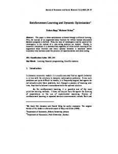
5.3 NCO-tracking results The solution model (18)-(24) is adapted using online measurements of X and S. The process is simulated for two realization of the uncertain parameter, Yx = 0.3 and Yx = 0.6. The performance of NCO tracking for these two cases is reported in Fig. 2 as dashed and dotted lines, respectively. 1 0.8 u [l/h]

0.6 0.4 0.2 0 0

2

4 t [h]

6

8

6 5

This paper presents a systematic procedure for deriving a solution model for the optimal operation of dynamic processes from a numerical solution. The solution model is used to track the NCO in order to retain a feasible and optimal operation under uncertainty. Even though the example used for illustration shows a fairly complex solution structure, the latter can be automatically detected and systematically converted into a solution model. Investigations of various uncertainty scenarios confirmed the robustness of the solution model. The suggested procedure still requires physical insight and experience to derive the NCO control law from the automatically detected solution structure. The objective of future work is to formalize this process in order to support the control system design to the extent possible.

S [g/l]

4 3

REFERENCES

2 1 0 0

2

4 t [h]

6

8

3 2.5 X [g/l]

2 1.5 1 Yx=0.3 Yx=0.6

0.5 0 0

2

4 t [h]

6

8

Fig. 2. Optimal profiles with NCO tracking for the perturbed parameter values Yx = 0.3, 0.6. It can be observed that the operation is feasible with respect to the state constraint on X, which is not the case with open-loop implementation of the nominal control to the perturbed process. The empirical model (24) is sufficiently accurate for the perturbations in Yx . The reference tracking on Arc 2 and Arc 5 has significantly improved the objective function. For Yx = 0.3, the control saturates on Arc 2. The objective function values using the open-loop implementation of the nominal control, the NCO tracking solution model and re-optimized control are given in Table 2. Using the solution model, the loss in optimality is very minimal, which can be further reduced by run-to-run updates. Table 2. Objective function values using different control strategies Yx 0.3 0.6

Open-loop infeasible infeasible

Solution model 5.47 6.73

Re-optimization 5.66 6.76

Bryson, A.E. and Y.-C. Ho (1975). Applied Optimal Control. Taylor & Francis. Bristol, PA. Kadam, J.V. and W. Marquardt (2004). Sensitivity-based solution updates in closed-loop dynamic optimization. In: Proc. of DYCOPS 7, Cambridge, USA (S.L. Shah and J.F. MacGregor, Eds.). Omnipress. Lee, J.H. and N.L. Ricker (1994). Extended Kalman filter based nonlinear model predictive control. Ind. Eng. Chem. Res. 33, 1530– 1541. Schlegel, M. and W. Marquardt (2004). Direct sequential dynamic optimization with automatic switching structure detection. In: Proc. of DYCOPS 7, Cambridge, USA (S.L. Shah and J.F. MacGregor, Eds.). Omnipress. Schlegel, M., K. Stockmann, T. Binder and W. Marquardt (2004). Dynamic optimization using adaptive control vector parameterization. Submitted to: Comp. Chem. Eng. Srinivasan, B. and D. Bonvin (2004). Dynamic optimization under uncertainty via NCO tracking: A solution model approach. In: Proc. BatchPro Symposium 2004 (C. Kiparissides, Ed.). pp. 17–35. Srinivasan, B., D. Bonvin, E. Visser and S. Palanki (2003a). Dynamic optimization of batch processes II. Role of measurements in handling uncertainty. Comp. Chem. Eng. 27, 27–44. Srinivasan, B., S. Palanki and D. Bonvin (2003b). Dynamic optimization of batch processes I. Characterization of the nominal solution. Comp. Chem. Eng. 27, 1–26. Zhang, Y., D. Monder and J.F. Forbes (2002). Real-time optimization under parametetric uncertainty: a probability constrained approach. J. Proc. Contr. 12, 373–389.