of conservation planning for three rare species in the Pacific. Northwest of the .... species survival as a controlled Dynamic Bayesian Network. (DBN, see e.g. ...
Dynamic Resource Allocation in Conservation Planning Daniel Golovin
Andreas Krause
Beth Gardner
Sarah J. Converse
Steve Morey
Caltech Pasadena, CA, USA
ETH Z¨urich Zurich, Switzerland
NCSU Raleigh, NC, USA
USGS Patuxent WRC Laurel, MD, USA
USFWS Portland OR, USA
Abstract Consider the problem of protecting endangered species by selecting patches of land to be used for conservation purposes. Typically, the availability of patches changes over time, and recommendations must be made dynamically. This is a challenging prototypical example of a sequential optimization problem under uncertainty in computational sustainability. Existing techniques do not scale to problems of realistic size. In this paper, we develop an efficient algorithm for adaptively making recommendations for dynamic conservation planning, and prove that it obtains near-optimal performance. We further evaluate our approach on a detailed reserve design case study of conservation planning for three rare species in the Pacific Northwest of the United States.
1
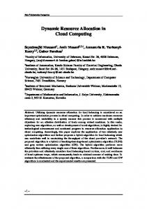
clairvoyant policy with knowledge of the future availability of resources. While there is a significant amount of both theoretical and applied work on conservation planning (which we review in §5), we are unaware of principled approaches that can solve such dynamic problems on a realistic scale. We further conduct a detailed computational study, evaluating our approach on the problem of conservation planning for three rare taxa (see Fig. 1(a)) in the Pacific Northwest of the United States. Our case study uses complex patch dynamics models (Hanski et al. 1996) for predicting persistence of species, using parameters elicited from an expert panel. Our results indicate that the optimized solutions outperform baselines, and that significant benefit can be derived from dynamic optimization.
Introduction
One key challenge in computational sustainability is to allocate resources in order to optimize long-term objectives. An archetypal application is conservation planning: managers recommend patches of land for conservation in order to achieve long-term persistence of endangered species. In this and similar applications, we typically have to make decisions over time: Financial resources (or other budgets) are periodically made available and should be used effectively. For example, every year, a certain budget may be available to support land conservation. The problem of how to optimally use this budget over time, facing uncertainty about the availability of future resources, is a challenging optimization problem. In this paper, we tackle this optimization problem using conservation planning as an important real-world example of such a decision task. We prove a surprising fact: Under some natural conditions, a simple policy, that in every round of the decision making process opportunistically allocates the budget given the current reserve and current resources, attains a performance which is competitive with the optimal c 2011, Association for the Advancement of Artificial Copyright Intelligence (www.aaai.org). All rights reserved. The authors’ full addresses are: Computing + Mathematical Sciences Dept., Caltech, 1200 E. California Blvd., Pasadena CA 91125, USA; Dept. of Comp. Sci., ETH Z¨urich, Universitaetsstrasse 6, 8032 Zurich, Switzerland; Dept. of Forestry and Environmental Resources, North Carolina State University, Raleigh NC 27695, USA; US Geological Survey, Patuxent Wildlife Research Center, 12100 Beech Forest Rd., Laurel MD 20708, USA; and US Fish and Wildlife Service, 911 N.E. 11th Avenue, Portland OR 97232, USA
2
Problem Statement
In the following, we formalize the problem of recommending parcels of land for conservation in order to maximize the persistence probability of a set I of species of interest. Let U be the set of all parcels (atomic units of land) in the geographic area. In many cases, such as in our case study described in §4.1, individual parcels may be too small to be managed as separate reserves, or to serve by themselves as a viable habitat for any particular species. Multiple, spatially adjacent parcels satisfying certain constraints (such as on the minimum total size) can form a patch P of land, which can be recommended for conservation (see also Fig. 1(b)). Let P be the set of all feasible patches. Our goal is to select one or more patches R ⊆ P as a reserve, in order to maximize the long-term persistence probability of the species. There are two main questions which we formalize in the following: 1) How can one quantify the benefit of a particular reserve for the purpose of sustaining the species, and 2) how can one effectively maximize this objective function?
2.1
Modeling Species Dynamics
Since we would like to ensure long-term survival of the species, we model the population dynamics among the parcels recommended for conservation. We use a patch dynamics model, i.e., employ Bernoulli random variables (i) Zp,t ∈ {0, 1} for i ∈ I, p ∈ U and t ∈ N to model whether species i is present (1) or absent (0) on parcel p at time t (i) (usually, in t years). The random vector Zt = [Zp,t ]i∈I,p∈U models the state of all parcels at time t. We model the
!"#$%&'&
R
!"#$%&(&
(a) Rare species considered in our case study
(b) Problem domain
(i)
Z1,t
(i)
Z1,t+1
Z2,t
(i)
Z2,t+1
(i) Z5,t
Z5,t+1
ηt
ηt+1
.. . .. .
(i)
.. .
(i)
.. .
(c) Controlled DBN
Figure 1: (a) The three taxa considered in our case study include the streaked horned lark (left), Taylor’s checkerspot (middle) and the Mazama pocket gopher (right). (b) Illustration of the problem domain. A map is partitioned into parcels (white cells), which are grouped into contiguous patches (red) of land. We model annual survival and colonization within selected patches. (c) Illustration of our metapopulation model.
species survival as a controlled Dynamic Bayesian Network (DBN, see e.g., Koller and Friedman [2009], and illustrated in Fig. 1(c)) with prior probability P [Z1 ] and transition probabilities P [Zt+1 | Zt , R, ηt ], i.e., the presence of species at time t + 1 depends on the presence at time t as well as which patches have been selected for conservation, and environmental conditions ηt (e.g., modeling the effect of a harsh winter). Hereby, the transition probability factorizes as i Y Y h (i) P [Zt+1 | Zt , R, ηt ] = P Zp,t+1 | Zt , R, ηt , (1) i
R∗ = arg max f (R),
(2)
R : c(R)≤b
that maximizes the persistence probability while P respecting a budget constraint b on the total cost c(R) = P ∈R c(P ).
p
and the environmental conditions η˜ = (η1 , . . . , ηT ) form a Markov chain. We needh to capture two aspects with the i (i) species survival model P Zp,t+1 | Zt , R, ηt : the fact that a population may or may not survive on its own within a parcel, and the fact that other populations of the same species may colonize it from nearby parcels. These distributions can be quite complex, and depend on habitat attributes of the parcels (e.g., vegetation, soils, etc.) as well as properties of the particular reserves (i.e., whether the contained parcels are separated by roads or waterways which hinder migration), and global properties (e.g., the likelihood of a harsh winter). In §4.1, we present details about the models used in our study.
2.2
Typically, each candidate patch P also has some cost c(P ) for reservation, e.g., its monetary cost, or the effort required to negotiate for its protection with the owners of its parcels. The goal of the static conservation planning problem then is to select a reserve
Static Reserve Design
Once we are able to model the population dynamics of the species, we would like to choose a reserve R to ensure longterm persistence. One natural goal is to define an objective function f (i) : 2P → R such that h i (i) f (i) (R) = P ∃P ∈ R, p ∈ P : Zp,T = 1 , quantifies the probability that species i is still present in at least one parcel in the reserve after some prediction horizon T (e.g., after 50 years). In order to ensure persistence of all species i ∈ I, a natural objective function is (typiP (i) cally in years) f (R) = w (R), where wi are a i∈I i f set of weights associated with the different species. In the following, w.l.o.g., we set wi = 1 for all species i, and thus f (R) effectively quantifies the expected number of species persisting after T timesteps.
2.3
The Dynamic Reserve Design Problem
In many natural reserve design settings, such as the one in our case study, it is not possible to conduct and implement a single optimization. Instead, we have to solve a sequential decision making process where over time new resources (patches of land and budget to spend) become available, and we have to dynamically determine recommendations based on our previous actions. Let Pt ⊆ P be the set of patches available for potential conservation at time t. Note that the sequence P1 , . . . , PT may not be known to us in advance; we may not know if or when a particular patch becomes a candidate for conservation. Let Rt denote the set of patches selected in the first t time steps. At every timestep, we are given a budget bt , and can select a collection R0 of additional patches from Pt of cost at most bt , taking into account which patches we have already selected, and set Rt = Rt−1 ∪ R0 . Unused budget from one timestep does not carry over to the next timestep. For clarity of presentation, here we consider the setting where conservation recommendations are made on a faster timescale than the patch dynamics. Thus, the goal is to plan the recommendation of patches to protect such that the final reserve1 RT maximizes the persistence probability f (RT ). Formally, we are interested in a conservation policy π : 2P × 2P × N × R+ → 2P , such that π(R, P 0 , t, b) specifies which patches to recommend at time t, given that we have already selected patches R, have the set P 0 of patches to choose from, and budget b to spend. A policy is feasible if, whenever π(R, P 0 , t, b) = R0 , then R0 ⊆ P 0 and c(R0 ) ≤ b. 1 Our model can be extended so that f also depends on the sequence of selections. We defer to an extended version of this paper.
For simplicity we focus on feasible stationary policies (i.e., π is independent of t). For fixed sequences of available patches and budgets P˜ = ˜ ˜b) ⊆ P be (P1 , . . . , PT ) and ˜b = (b1 , . . . , bT ), let R(π, P, the final reserve assembled at time T . We say a policy is α-competitive for some α ∈ [0, 1] if for all P˜ and ˜b we have ˜ ˜b)) ≥ α max f (R(π 0 , P, ˜ ˜b)). f (R(π, P, 0 feasible π
(3)
We call the problem of efficiently determining an αcompetitve policy the dynamic reserve design problem. Note that α-competitiveness is a very strong notion: It requires that the selected reserve be nearly as good as a reserve that could be selected by a clairvoyant policy, one that gets to know the sequences P˜ and ˜b in advance.
3
Optimization Algorithm
Even for a single timestep, selecting the set of patches that maximizes the survival probability is an NP-hard optimization problem2 . Despite this hardness, in the following, we present an efficient policy that exploits certain structural features for dynamic conservation planning.
3.1
Problem Structure.
We will prove that if species do not colonize between separate patches, then we can guarantee near-optimal solutions. Formally, we require that P [ZP,t+1 | Zt , R, ηt ] = P [ZP,t+1 | ZP,t , [P ∈ R], ηt ] , (4) where ZP,t is the state of all parcels in patch P at time t, and [P ∈ R] refers to a binary variable indicating whether P ∈ R. Thus, the patch dynamics for patch P depend only on the state of all parcels in patch P , whether P is included in reserve R, and environmental conditions η. This condition is naturally satisfied if the candidate patches are spatially separated, such that natural barriers blocking colonization are likely to exist. Note that crucially we do model colonization between parcels within one patch. Under condition (4), it can be shown that the function f (R) satisfies a natural diminishing returns condition: It holds that f (R ∪ {P }) − f (R) ≥ f (R0 ∪ {P }) − f (R0 ) whenever R ⊆ R0 . Set functions with this property are called submodular3 (c.f., Nemhauser, Wolsey, and Fisher, 1978). Furthermore, it holds that f is monotonic, i.e., f (R) ≤ f (R0 ) whenever R ⊆ R0 .
Proposition 1. Suppose Condition (4) holds. Then the function f : 2P → R is a monotonic submodular function.
Proof. Fix environmental conditions sequence η˜ and initial states for all parcels z0 . Using the factorial structure of the DBN (1) and assumption (4), Q one can show by induction on T that P [ZT | z0 , R, η˜] = P P [ZP,T | z0 , R, η˜]. Thus h i Y (i) P ∃P ∈ R, p ∈ P : Zp,T = 1 | z0 , R, η˜ = 1− qP,i (z0 , η˜), P ∈R
2
Using a reduction from the max-k-cover problem. Note that without this condition, submodularity can be violated as shown by Sheldon et al. [2010]. 3
h i (i) where qP,i (z0 , η˜) := P ∀p ∈ P : Zp,T = 0 | z0 , R, η˜ . Q One can see that g(R; z0 , η˜) := 1 − P ∈R qP,i (z0 , η˜) is monotonic submodular in R. Since nonnegative linear combinations preserve submodularity, the objective f (R) = R g(R; z0 , η˜)dP [z0 , η˜] is monotonic submodular. Note that this result is rather general: In particular, it supports modeling complex relationships among species (such as symbiosis or predator-prey relationships), and arbitrary (potentially correlated) priors on the initial occupancy P [Z0 ].
3.2
Solving the Static Problem
For submodular functions, a seminal result of Nemhauser, Wolsey, and Fisher [1978] states that a simple greedy algorithm, which starts with R0 = ∅, and iteratively sets R`+1 = R` ∪ {arg maxP f (R` ∪ {P })} achieves a nearoptimal solution in the case where the cost of all patches is uniform: It holds that f (Rk ) ≥ (1 − 1/e) max|R|≤k f (R). Using a more complex algorithm which combines partial enumeration with greedy selection, the same guarantee can be obtained for arbitrary nonnegative costs (c.f., Sviridenko, 2004). This algorithm can hence be used to obtain a nearoptimal solution to the static reserve design problem (2).
3.3
Opportunistic Dynamic Selection
The dynamic problem (3) appears much more demanding: In principle, to do well, one may need to plan ahead based on which patches may become available at future timesteps, but there is a combinatorial number of possibilities. In the following, perhaps surprisingly, we show that one can do well purely by opportunistically selecting patches at each round, disregarding the potential availability of patches in the future. Formally, in round t the algorithm implements the policy πopp (Rt−1 , Pt , t, bt ) = arg max ft (R0 ), (5) 0
R0 ⊆Pt :c(R0 )≤bt R0 ) − f (Rt−1 ) is
where ft (R ) := f (Rt−1 ∪ the residual objective at round t. We have the following result: Theorem 2. The policy πopp is 1/2-competitive, that is ˜ ˜b)) ≥ 1/2 · max f (R(π, P, ˜ ˜b)). f (R(πopp , P, feasible π
If we use a β-approximate implementation of πopp , the resulting policy is β/(1 + β) competitive. Note that if f is submodular, then so is ft . Thus, problem (5) is an instance of the static design problem (2) and thus we can use the algorithm analyzed by Sviridenko [2004] e−1 for optimization (β = 1− 1e ), resulting in a 2e−1 -competitive policy. Thus, this simple opportunistic policy obtains at least 38.7% of the reward of any feasible policy, even clairvoyant ones (which know when each patch will become available). Proof Sketch. Suppose the sequences P˜ and ˜b are given in advance. Then the problem of developing an optimal policy can be reduced to the problem of maximizing a submodular function subject to a simple partition matroid constraint with the base set F1 ∪ · · · ∪ FT , where Ft = {R ⊆ Pt : c(R) ≤ bt }. The (approximate) opportunistic policy can then be seen to be the (approximate) locally-greedy algorithm applied to this problem instance, and the result follows from the analysis of Goundan and Schulz [2007].
● ●
●
● ●
● ●
● ●
100
200 300 400 Parcel Size (Acres)
500
dynamic optimization
1.5
dynamic by area a priori optimization
1
random
0.5 0 0
10
20 30 40 50 Budget per round (km2)
60
2.5
2.5 2 dynamic optimization dynamic by area random
1.5 1
a priori optimization
0.5 0 0
(d) Dynamic reserve design
2
4
6
8
10
Optimized
2
by area
1.5 random 1 0.5
(b) Fitted survival probabilities for SHL Expected number of persist. species
2
Expected number of surviving species
Annual Patch Survival Probability 0.2 0.4 0.6 0.8 1.0 0.0
●
2.5 Expected number of persist. species
Exp. # of species persist. after 10 rounds
● ●
●
0
(a) Elicited survival probabilities for SHL
● ● ●
● ● ● ● ●
●
0 0
10
20
30 40 Budget (km2)
50
60
(c) Static reserve design 2.5 2
dynamic optimization dynamic by area
1.5 random
1
a priori optimization
0.5 0 0
2
4
6
8
10
Round
Round
(e) Dynamic reserve design
(f) Dynamic design with failures
Figure 2: Experimental results.
4 4.1
Experimental Results
Reserve Design Case Study
We are conducting a computational study in collaboration with the US Fish and Wildlife Service Washington Office, in Washington State, USA. The eventual goal of this collaboration is to develop a tool that will facilitate decision-making about assembly of a reserve adequate to protect three Federal Candidate taxa inhabiting a remnant prairie ecosystem in the South Puget Sound region. The target species are Taylor’s checkerspot (TCS; Euphydryas editha taylori), Mazama pocket gopher (MPG; Thomomys mazama), and streaked horned lark (SHL; Eremophila alpestris strigata). As part of this effort, we held elicitation workshops to garner the input of biologists with expertise on the target taxa and the South Puget Sound prairie ecosystem. The goal of these workshops was to parameterize patch dynamics models for each of the species. Substantial uncertainty currently exists about the ecological processes governing the behavior of populations of the target taxa. Our intent during the workshops was to formally capture this uncertainty, via inter-expert variation, so that it could be reflected in the predictive patch dynamics models, and ultimately conservation recommendations could be obtained that are robust to this uncertainty; to do so we used a modified Delphi process for expert elicitation (c.f., Vose, 1996). Fig. 2(a) presents an example annual survival curve elicited from an expert for SHL, and Fig. 2(b) shows a fit based on inputs from multiple experts. The primary objective is to maximize persistence probability after 50 years for each of the candidate taxa. We first identified the set of land parcels in appropriate portions of the Washington counties of
Grays Harbor, Lewis, Mason, Pierce, and Thurston (including Ft. Lewis Army Base): These are located at least partially on appropriate prairie soil types; are classified by county surveyors offices as undeveloped, agriculture, open space, or forest; and are at least 5 acres in size and can be combined with adjacent qualifying parcels to assemble a contiguous patch that is at least 100 acres in size. We also obtained spatial data on soil types, elevation, vegetation type, and barriers (selected roads and water ways), which were processed using ArcGIS 9.3 (Environmental Systems Research Institute 2008) to determine the habitat properties of each parcel and the barriers hindering colonization. We use parametric models h for the stochastic i aspects in the (i) patch dynamics model P Zp,t+1 | Zt , R, ηt . Due to space limitations, we only provide an overview here. 1. Annual Survival. Annual survival of a population in a parcel depends on the usable habitat size. This dependence of the survival probability on habitat size, as well as the factors determining habitat size itself, were elicited. Since ecological processes vary over time, and environmental conditions (e.g., a harsh winter, the spread of a disease) can affect survival, we estimate a spatially correlated reduction or increase in the effective habitat area by using a Gaussian process model with exponential kernel; the components of this model (e.g., the degree of annual variance and spatial correlation in variance), were also elicited from experts. 2. Colonization. The probability of species colonization is modeled using a parametric function of the source parcel habitable area (annually-varying, as described above), the
distance between source and target parcel, and environmental conditions using models from the literature where available (for the Taylor’s checkerspot; see Hanski et al. [1996]) or based on expert elicitation. Barriers (interstates, major highways, and water bodies) reduce migration probability to varying degrees for TCS and MPG. Prior distributions on the parameters of these stochastic components were elicited from the expert panel. In order to capture the variation, we conduct multiple simulations, with parameters sampled from the estimated prior distributions. For conservation cost, we use the size (in km2 ) of each parcel.
4.2
Experimental Setup
We generate contiguous candidate patches from the parcels by a region growing process, which picks a random parcel as seed, and then iteratively grows the patch up to a random size. This growth process is randomly biased to avoid complex boundaries. Using this procedure we generate 10,000 candidate patches for selection. To evaluate the objective function, we generate 100 random samples from the DBN (1). To avoid overfitting, two thirds of those are used for optimization (as done, for example by Sheldon et al. [2010] for a similar problem), and the quality of the solutions are evaluated against the remaining one third. As noted by Sheldon et al. [2010], the advantage of this procedure is that preprocessing can be used to drastically speed up computation and bounds on the generalization error can be obtained. Further, instead of using the algorithm described by Sviridenko [2004] for solving Problem (2), we use a faster algorithm of Leskovec et al. [2007] that also carries theoretical guarantees.
4.3
±
Optimization Results
In our experiments, we mainly aim to investigate the following questions: 1. How much better do optimized solutions perform compared to simple baselines? 2. How much can be gained from dynamic optimization? We first conduct experiments on the static reserve design problem (2). We vary the budget from 0 to 60 km2 , and compare the optimized reserves with random selection, as well as selecting patches according to decreasing area. Fig. 2(c) presents the results. Note that optimized selection drastically outperforms the baselines. Running time for this problem instance is less than 45 seconds on a standard 2.66 GHz, 4 GB configuration. Fig. 3 shows a solution obtained for b = 10km2 . We then evaluate our near-optimal policy for dynamic conservation planning. We randomly partition the set of all patches into T = 10 different subsets P1 , . . . , PT . In our experiment, we vary the budget bt which is made available in each round from 0 to 60 km2 . We then opportunistically select patches each round, either by optimization, in decreasing order of area, or at random. All experiments are repeated, and results averaged, over 10 random trials. In order to estimate the benefit of dynamic selection, we also compare against another baseline, where we a priori (approximately) optimize a fixed reserve (having access to all patches and the entire budget), and then, for this fixed solution, pick patches in the first round in which they become available.
0 5 10
20 Kms
Figure 3: Selected patches (red) for one solution, with b = 10km2 . In Fig. 2(d) we plot the expected number of persistent species (after 50 years) after ten rounds of selection. Note that the dynamically optimized solution outperforms the baselines. Note that even after all ten rounds (i.e., after all patches were made available) the sequential solution outperforms the a priori solution. The reason is that the static a priori optimization is not aware of the per-round budget constraints, and therefore may not be able to select some patches as they become available. Fig. 2(e) plots, for a fixed budget per round, the value of the reserves f (Rt ) during the ten rounds of selection. Note that the dynamic approaches drastically outperform the a priori selection. Lastly, we also perform an experiment, where the algorithms at each round attempt to recommend some patches for conservation. However, these recommendations may fail (i.e., cannot be implemented due to external constraints). Here we consider failures that happen randomly, with probability 0.5 independently for each patch4 . Fig. 2(f) presents the result of this experiment. Note that in contrast to Fig. 2(e), here the dynamic approaches achieve much better performance than the static baseline. The reason for this is that the dynamic approaches may be able to substitute an “important” failed selection by a similar alternative that becomes available in a later round.
5
Related Work
Conservation planning. There are several powerful tools available for conservation planning, including Marxan (Ball, Possingham, and Watts 2009) and Zonation (Moilanen and Kujala 2008). However, none of those tools currently implements complex patch dynamics models of species persistence. Also, they do not provide guarantees of (near-) optimality. Perhaps closest in spirit to our work is an approach by Sheldon et al. [2010]. They propose a network optimization approach with applications to conservation planning. In their approach, they model the population behavior using 4
Our theoretical analysis holds even in this more general setting, relying on a generalization of submodularity to adaptive policies (Golovin and Krause 2010). We omit details due to space limitations.
the independent cascade model of Goldenberg, Libai, and Muller [2001]. One particular aspect that they consider is the non-submodularity of the reserve design problem in absence of Condition 4. They propose an approach based on MixedInteger Programming (MIP) to overcome limitations of the greedy algorithm. However, their work does not handle the dynamic aspects of conservation planning that are the focus of this paper. The independent-cascade model is essential to their approach, and it seems difficult to use it to model complex interactions between species (such as symbiosis or predator-prey relationships), or more complex population dynamics (beyond presence-only population models), which all can be handled by our approach. Furthermore, in most of their experiments conducted on a real reserve design case study, the non-greedy network design approach based on MIP performs comparably to the greedy approach, providing further evidence about the appropriateness of Condition 4. We consider the development of principled dynamic planning approaches that do not rely on Condition 4 an interesting direction of future work. Submodular optimization. The problem of adaptively optimizing submodular functions has been studied by Golovin and Krause [2010]. However, their approach is not known to provide competitiveness guarantees such as those of Theorem 2, where the set of available actions changes over time. Streeter and Golovin [2008] provide an algorithm for the problem of online maximization of submodular functions. In their setting, the decision maker chooses a different set at each round, maximizing the sum of objective values attained over time. The conservation planning problem does not fit into this framework, since we are interested in building a single set of reserves by adding patches over time. Another related problem is submodular optimization over data streams, as studied by Gomes and Krause [2010]. However, their algorithm requires that it is possible to unselect already selected items (patches), which may not be possible in the conservation planning problem. Lastly, the problem studied in this paper is also related to the submodular secretary problem, studied by Bateni, Hajiaghayi, and Zadimoghaddam [2010]. However, their guarantees require that the sequence of elements that become available over time is randomly permuted. Our approach does not make any assumption about the order in which patches become available.
6
Conclusion
We considered the problem of protecting rare species by recommending patches of land for conservation. Our approach employs a detailed probabilistic patch dynamics model in order to ensure long-term persistence of taxa in the selected reserves. Our model can handle complex annual survival and colonization patterns, as well as interactions among species (though not demonstrated here). In order to cope with changing availability of patches, we proposed an opportunistic policy for dynamically making recommendations. We proved the surprising result that this simple opportunistic policy is competitive with a clairvoyant solution that is informed in advance of the budget in each timestep and when each patch will be available. We conducted a detailed case study of conservation planning for three rare taxa in the Pacific Northwest
of the United States. Our results indicate that the optimized solutions drastically outperform simple baselines, and that significant benefit can be obtained from dynamic planning. We believe that our results provide interesting insights for dynamic/adaptive optimization, and could be useful for other applications such as influence maximization over networks. Acknowledgments. This research was partially supported by ONR grant N00014-09-1-1044, NSF grants CNS-0932392 and IIS-0953413, the Caltech Center for the Mathematics of Information, and by the US Fish and Wildlife Service. We thank J. Bakker, J. Bush, M. Jensen, T. Kaye, J. Kenagy, C. Langston, S. Pearson, M. Singer, D. Stinson, D. Stokes, and T. Thomas for their contributions.
References Ball, I.; Possingham, H.; and Watts, M. 2009. Spatial conservation prioritisation: Quantitative methods and computational tools. Oxford University Press. chapter Marxan and relatives: Software for spatial conservation prioritisation. Bateni, M. H.; Hajiaghayi, M.; and Zadimoghaddam, M. 2010. The submodular secretary problem and its extensions. In APPROX. Environmental Systems Research Institute. 2008. ArcGIS 9.3 users manual. Technical report, ESRI. Goldenberg, J.; Libai, B.; and Muller, E. 2001. Talk of the network: A complex systems look at the underlying process of word-of-mouth. Marketing Letters 12(3):211–223. Golovin, D., and Krause, A. 2010. Adaptive submodularity: Theory and applications in active learning and stochastic optimization. CoRR abs/1003.3967v3. Gomes, R., and Krause, A. 2010. Budgeted nonparametric learning from data streams. In ICML. Goundan, P. R., and Schulz, A. S. 2007. Revisiting the greedy approach to submodular set function maximization. Technical report, Massachusetts Institute of Technology. Hanski, I. A.; Moilanen, A.; Pakkala, T.; and Kuussaari, M. 1996. The quantitative incidence function model and persistence of an endangered butterfly metapopulation. Conservation Biology 10. Koller, D., and Friedman, N. 2009. Probabilistic Graphical Models. The MIT Press. Leskovec, J.; Krause, A.; Guestrin, C.; Faloutsos, C.; VanBriesen, J.; and Glance, N. 2007. Cost-effective outbreak detection in networks. In KDD. Moilanen, A., and Kujala, H. 2008. ZONATION: Spatial conservation planning framework and software. www.helsinki.fi/bioscience/ConsPlan. Nemhauser, G. L.; Wolsey, L. A.; and Fisher, M. L. 1978. An analysis of approximations for maximizing submodular set functions - I. Math. Prog. 14(1):265–294. Sheldon, D.; Dilkina, B.; Elmachtoub, A.; Finseth, R.; Sabharwal, A.; Conrad, J.; Gomes, C.; Shmoys, D.; Allen, W.; Amundsen, O.; and Vaughan, B. 2010. Maximizing the spread of cascades using network design. In UAI. Streeter, M., and Golovin, D. 2008. An online algorithm for maximizing submodular functions. In NIPS. Sviridenko, M. 2004. A note on maximizing a submodular set function subject to knapsack constraint. Operations Research Letters 32:41–43. Vose, D. 1996. Quantitative Risk Analysis: A Guide to Monte Carlo Simulation Modeling. John Wiley and Son.