Dynamic Response Characterization of Complex ...

Dynamic Response Characterization of Complex Systems through Operational Identification and Dynamic Substructuring

An application to gear noise propagation in the automotive industry

PROEFSCHRIFT

ter verkrijging van de graad van doctor aan de Technische Universiteit Delft, op gezag van de Rector Magnificus prof. dr. ir. J.T. Fokkema, voorzitter van het College van Promoties, in het openbaar te verdedigen op woensdag, 18 maart 2009 om 12:30 uur

door

Dennis DE KLERK werktuigkundig ingenieur, geboren te Meppel, Nederland.

Dit proefschrift is goedgekeurd door de promotor: Prof. dr. ir. D.J. Rixen. Samenstelling promotiecommissie: Rector Magnificus Prof. dr. ir. D.J. Rixen Prof. dr. ir. D.J. Ewins Prof. dr. ir. P. Sas Prof. dr. ir. A. de Boer Prof. dr. ir. A.C.W.M. Vrouwenvelder Prof. Dr. ir. E. Balmes Prof. Dr. ir. P. Zeller

voorzitter Delft University of Technology Imperial College of Science and Technology Katholieke Universiteit Leuven University of Twente Delft University of Technology Ecole Centrale Paris Technische Universit¨ at M¨ unchen / BMW AG

ISBN 978-90-9024095-4 c Copyright 2009 by D. de Klerk – All rights reserved – No part of the material protected by this copyright notice may be reproduced or utilized in any form or by any means, electronic or mechanical, including photocopying, recording or by any information storage and retrieval system, without the prior written permission of the author.

ii

To my Grandfather and beloved Nynke

iii

Preface From the winter of 2004 onwards, BMW gave me the opportunity to perform a Ph.D. project in their research & development facility. During this period of time I was able to apply skills learned in the past and obtain new ones, specifically in the fields of experimental methods / techniques, and in the field of combined experimental and numerical structural analysis. Although a Ph.D. thesis carries only one name, it is actually a work of many. Colleagues, university staff, family and friends made contributions to my work in various ways, allowing me to present this thesis at it’s present level. First of course a special thanks to prof. dr. ir. D.J. Rixen who was of great help and inspiration throughout the project. Daniel, I admire your remarkable creativity, your passion for educating and your endless energy. Furthermore, this thesis would not have been at it’s present level without the enthusiastic work of A.H.H. van Tienhoven [114], J. de Jong [26], M. Brunner [10], C.L. Valentin [113], F. Pasteuning [87] and S.N. Voormeeren [116]. I would like to thank you all for your companionship, dedicated work & the great fun we had doing it! I would also like to take this the opportunity to thank all the colleagues at BMW who were of great help, great support and made this project possible in the first place. Other companies who also added to this work and therefore deserve mentioning are M¨ ullerBBM-VAS GmbH, Polytec GmbH, Kistler GmbH, Vibracoustic GmbH, CADCON & SDtools. Finally I would like to thank my family and especially my future wife Nynke for their support and loving. February 19, 2009,

D. de Klerk

iv

Abstract Dynamic Response Characterization of Complex Systems through Operational Identification and Dynamic Substructuring This thesis deals with new methods, which can determine the dynamic response of a complex system identified in operation, based on the knowledge of its subsystem dynamics and excitation. In the first part of this thesis, the identification of component excitation and its transmission into the total system will be addressed. The identification of the internal component excitation is performed on a test bench, on which equivalent forces at the component interface to the test setup are measured. The total system’s response is calculated on the knowledge of its dynamic properties from the component interface onwards. It is shown that physically correct responses for the systems in front of the component’s interface can be calculated. A compensation technique is also outlined to eliminate possible test bench influences. In this thesis, this first approach is called the Gear Noise Propagation (GNP) method, which can be seen as a special class of the well known Transfer Path Analysis (TPA) method. The method could be partially validated on the vibration propagation of a Rear Axle Differential (RAD) in a vehicle, also showing that test bench influences can be minimized in real life applications. In the second part, a new experimental strategy is developed, which enables the identification of systems in operation. In this thesis the method is referred to as the Operational System Identification (OSI) method. It is shown that the signal processing involved yields better FRF estimates than the classical Cross Power Spectrum (CPS) and Auto Power Spectrum (APS) averaging technique. In addition the method has been successfully validated by comparison with the Principle Component Analysis (PCA) method on a test object. Application of the method to an operating vehicle reveals some interesting dependencies of its system dynamics on temperature and applied engine torque. The third part of this thesis deals with methods which improve coupling results in experimental Dynamic Substructuring (DS) applications. First a general framework is presented with which different kinds of substructuring methods developed in the past can be classified. Thereafter methods which improve subsystem connectivity and compensate for shaker’s side force excitation are presented. An error propagation method is also developed with which the uncertainty on the coupled system FRF can be determined, based on the uncertainties of its subsystems. Validation of the new methods on a vehicle’s v

Rear Axle system shows good improvements could be achieved. In addition it will be shown that random errors on the subsystem FRF only play a significant role for very lightly damped systems. Yet in general, bias errors in the subsystem measurement and in the subsystem coupling definition are found to yield most of the discrepancies in experimental DS. Combinations between the methods developed in the first three parts are made in the fourth part of this thesis. It is shown that experimental DS is an efficient tool to identify influences of component operational parameters on the total systems performance. Furthermore it is shown that DS is helpful in sensitivity analysis and simple component design.

Dennis de Klerk, February 19, 2009

Samenvatting Karakterizeren van dynamische reacties van complexe systemen door middel van operationele identificatie en Dynamic Substructuring Dit proefschrift behandelt methodes waarmee het acoustische antwoord van een complex apparaat bepaald kan worden met behulp van identificatie methodes in bedrijfstoestand en kennis van de eigenschappen van onderdelen en onderdeel excitaties. In het eerste deel van dit proefschrift wordt de identificatie van onderdeel excitatie en de daaruit volgende trillingsoverdracht in het totale systeem behandeld. De identificatie van de eigenlijke excitatie van het onderdeel wordt op een meetopstelling uitgevoerd, waarbij equivalente krachten op de verbinding tussen meetopstelling en onderdeel bepaald worden. De reactie van het apparaat zelf wordt daarna berekend met behulp van de acoustische eigenschappen van de interface tussen onderdeel en apparaat. In dit proefschrift wordt aangetoond dat de berekende responsie physisch correct zijn voor alle onderdelen na de interface. In dit proefschrift wordt deze methode met de Gear Noise Propagation (GNP) methode aangeduid, waarbij ze als een speciale klasse van de bekende Transfer Path Analysis (TPA) methode gezien kan worden. De methode kon deels gevalideerd worden voor een differentieel van een voertuig. Hierbij wordt tevens aangetoond, dat de invloeden van de meetopstellingen geminimaliseerd kunnen worden. In het tweede deel wordt een nieuwe experimentele techniek ontwikkeld, waarmee de eigenschappen van apparaten of onderdelen in bedrijfstoestand bepaald kunnen worden. In dit proefschrift wordt deze techniek als Operational System Identification (OSI) methode getypeerd. Er wordt aangetoond dat de signaal verwerking van deze techniek tot betere Frequency Response Functions (FRF) leidt dan de klassieke methode met Cross Power Spectrum (CPS) en Auto Power Spectrum (APS) middeling. De methode wordt succesvol vi

gevalideed door een vergelijking met de Principle Component Analysis (PCA) methode. Toepassing van de OSI methode op een voertuig in bedrijfstoestanden toont enkele interessante afhankelijkheden ten aanzien van temperatuur en geappliceerd aandrijfmoment aan. In het derde deel van dit proefschrift worden methodes ontwikkeld ter verbetering van koppelingsresultaten bereikt met de experimentele Dynamic Substructuring (DS) methode. Allereerst wordt een algemeen raamwerk gepresenteerd waarmee de verschillende substructuring methodes, ontwikkeld in het verleden, geclassificeerd kunnen worden. Daarna worden methodes gepresenteerd die de koppelingsmechaniek tussen substructures verbetert en zijkrachten van shaker excitaties compenseert. Er wordt ook een fouten analyse opgesteld waarmee de onzekerheid op subsysteem FRFs vertaald kan worden naar de onzekerheid op de gekoppelde FRFs. Validatie van de methode op een voertuig achteras laat zien dat er goede verbeteringen behaald konden worden. Daarnaast wordt aangetoond dat ruis op de subsysteem FRFs enkel een significante rol speelt voor licht gedempte systemen. Maar in het algemeen kan gesteld worden dat bias fouten op de subsysteem metingen en in de subsysteem koppelingsdefinitie tot de grootste fouten leiden. Combinaties tussen de verschillende methodes in de eerste drie delen worden beschreven in het vierde deel van dit proefschrift. Daarbij toont de experimentele DS methode zichzelf als een effici¨ente tool om de invloeden van componenten eigenschappen op het gekoppelde systeem hebben. Daarnaast wordt ge¨ıllustreerd dat DS een handige methode is om sensitivity analyses uit te voeren.

Dennis de Klerk, February 19, 2009

vii

viii

Contents Preface

iv

Abstract Introduction Research Context . . . . . . . . . . . Current State of Technology . . . . . Scientific Challenge & Thesis Topics Personal Contributions . . . . . . . . Thesis Outline . . . . . . . . . . . .

v

. . . . .

. . . . .

. . . . .

. . . . .

. . . . .

. . . . .

. . . . .

. . . . .

. . . . .

. . . . .

. . . . .

. . . . .

. . . . .

. . . . .

. . . . .

. . . . .

. . . . .

. . . . .

. . . . .

. . . . .

. . . . .

. . . . .

. . . . .

. . . . .

. . . . .

. . . . .

. . . . .

. . . . .

. . . . .

Part I: From Test Bench to System Response Estimates 1 The 1.1 1.2 1.3 1.4 1.5 1.6

13

Gear Noise Propagation Method Theory . . . . . . . . . . . . . . . . . . . . . . . . . . . . . . . . . . . . . Compensation for Nonrigid Test Benches . . . . . . . . . . . . . . . . . The GNP Method Extended for Nonmeasurable Interface FRFs . . . . . Including Operational Parameters & Nonlinearities in the GNP Method Comparison with the Transfer Path Analysis (TPA) Method . . . . . . . Summary . . . . . . . . . . . . . . . . . . . . . . . . . . . . . . . . . . .

2 Measurements, Results & Validation 2.1 Validation Strategy . . . . . . . . . . . . . . . . . . . . . . . . . . 2.2 The GNP Application - Measurements & Results . . . . . . . . . 2.2.1 RAD Test Bench Measurement . . . . . . . . . . . . . . . 2.2.2 Nonoperating Vehicle FRF Measurement . . . . . . . . . 2.2.3 Vehicle Dynamometer Measurement . . . . . . . . . . . . 2.3 Gear Force Independency on Gearbox Quasi-Static Deformation 2.4 Gear Force Independency on Gearbox Dynamic Motion . . . . . 2.5 GNP Synthesis & Validation . . . . . . . . . . . . . . . . . . . . 2.6 Conclusion . . . . . . . . . . . . . . . . . . . . . . . . . . . . . .

. . . . . . . . .

3 3 4 7 9 10

. . . . . . . . .

. . . . . . . . .

. . . . . . . . .

. . . . . .

. . . . . .

. . . . . .

. . . . . .

. . . . . .

. . . . . .

15 16 22 24 28 29 32

. . . . . . . . .

. . . . . . . . .

. . . . . . . . .

. . . . . . . . .

. . . . . . . . .

. . . . . . . . .

35 35 38 39 40 41 43 44 46 47

Part II: System Identification in Motion

51

3 Identification of an Operating System’s Structural Dynamics 3.1 Introduction . . . . . . . . . . . . . . . . . . . . . . . . . . . . . . . . . . . . . . . . 3.2 The OSI Measurement Procedure . . . . . . . . . . . . . . . . . . . . . . . . . . . .

53 53 54

ix

3.3 3.4 3.5

Measurement Equipment & Shaker Signal Processing . . . . . . . . . . . . . . . . . Validation of the OSI Method . . . . . . . . . . . . . . . . . . . . . . . . . . . . . . Estimate of the Operational Residue on the FRF . . . . . . . . . . . . . . . . . . .

4 Application of the OSI 4.1 Measurement . . . . 4.2 Results & Discussion 4.3 Conclusion . . . . .

Method on an Operating Vehicle . . . . . . . . . . . . . . . . . . . . . . . . . . . . . . . . . . . . . . . . . . . . . . . . . . . . . . . . . . . . . . . . . . . . . . . . . . . . . . . . . . . . . . . . . . . . . . . . . . . . . . . . .

Part III: Assembling Pieces of the Puzzle 5 A General Framework for Dynamic Substructuring 5.1 Random Walk in History . . . . . . . . . . . . . . . . 5.2 A General Framework for Dynamic Substructuring . . 5.3 Classification of FBS Methods . . . . . . . . . . . . . . 5.4 Difficulties in Experimental DS . . . . . . . . . . . . . 5.5 Conclusion . . . . . . . . . . . . . . . . . . . . . . . .

59 61 64 67 67 68 70

73 . . . . .

. . . . .

. . . . .

. . . . .

. . . . .

. . . . .

. . . . .

. . . . .

. . . . .

75 76 79 88 90 93

6 Coupling Procedure Improvement & Uncertainty Quantification 6.1 Defining Subsystem Connectivity . . . . . . . . . . . . . . . . . . . . 6.1.1 Theory of the EMPC & IDM Filtration Method . . . . . . . 6.2 Compensation for Side Forces in FRF Estimates . . . . . . . . . . . 6.2.1 Theory of the SFC Method . . . . . . . . . . . . . . . . . . . 6.2.2 Verification of the SFC method . . . . . . . . . . . . . . . . . 6.2.3 Results . . . . . . . . . . . . . . . . . . . . . . . . . . . . . . 6.2.4 Summary . . . . . . . . . . . . . . . . . . . . . . . . . . . . . 6.3 Uncertainty Propagation in Dynamic Substructuring . . . . . . . . . 6.3.1 Theory of Uncertainty Propagation . . . . . . . . . . . . . . . 6.3.2 Uncertainty Propagation in Subsystem FRF Estimation . . . 6.3.3 Uncertainty Propagation in the Coupling Procedure . . . . . 6.3.4 Interesting Observations . . . . . . . . . . . . . . . . . . . . . 6.3.5 Summary . . . . . . . . . . . . . . . . . . . . . . . . . . . . .

. . . . . . . . . . . . .

. . . . . . . . . . . . .

. . . . . . . . . . . . .

. . . . . . . . . . . . .

. . . . . . . . . . . . .

. . . . . . . . . . . . .

. . . . . . . . . . . . .

. . . . . . . . . . . . .

95 96 96 100 101 103 104 106 107 109 112 114 115 117

7 Validation of the Experimental DS Method in Vehicle Dynamics 7.1 Coupling Variants & Strategy . . . . . . . . . . . . . . . . . . . . . . 7.2 Subsystem Interface Definition & Modeling . . . . . . . . . . . . . . 7.3 Numerical Substructure Modeling & Validation . . . . . . . . . . . . 7.3.1 Modeling of the Rear Axle Differential . . . . . . . . . . . . . 7.3.2 Modeling of the Rear Axle Carrier . . . . . . . . . . . . . . . 7.3.3 Modeling of the Rubber Mountings . . . . . . . . . . . . . . . 7.4 Experimental Substructure Modeling & Validation Measurements . . 7.4.1 Bodywork Substructure Measurement . . . . . . . . . . . . . 7.4.2 Vehicle Substructure Measurement . . . . . . . . . . . . . . . 7.4.3 Validation Measurements . . . . . . . . . . . . . . . . . . . . 7.5 Coupling Results . . . . . . . . . . . . . . . . . . . . . . . . . . . . . 7.5.1 Results of the Subsystem Connectivity Variants . . . . . . . . 7.5.2 Results of the Side Force Compensation Method . . . . . . . 7.5.3 Results of the Uncertainty Propagation Method . . . . . . . . 7.5.4 Results of the RAC – BW Coupling . . . . . . . . . . . . . .

. . . . . . . . . . . . . . .

. . . . . . . . . . . . . . .

. . . . . . . . . . . . . . .

. . . . . . . . . . . . . . .

. . . . . . . . . . . . . . .

. . . . . . . . . . . . . . .

. . . . . . . . . . . . . . .

. . . . . . . . . . . . . . .

119 119 122 127 127 128 131 136 136 139 140 146 146 149 150 155

x

. . . . .

. . . . .

. . . . .

. . . . .

. . . . .

. . . . .

. . . . .

7.6

7.5.5 Results of the RAD – RAC – BW Coupling . . . . . . . . . . . . . . . . . . 157 7.5.6 Results of the RAD – Vehicle Coupling . . . . . . . . . . . . . . . . . . . . 159 Conclusion . . . . . . . . . . . . . . . . . . . . . . . . . . . . . . . . . . . . . . . . 159

Part IV: Combining all three Ingredients 8 Combining the GNP, OSI & DS Method in Vehicle Design 8.1 Combination of the GNP & OSI Method . . . . . . . . . . . . . . . . . 8.2 Influence of Rubber Mounting Temperature on the Vehicle Properties 8.3 Sensitivity of the Vehicle FRF on the RAD’s Mass . . . . . . . . . . . 8.4 Design of a Tuned Mass Damper for an Operating Vehicle . . . . . . .

163 . . . .

. . . .

. . . .

. . . .

. . . .

. . . .

. . . .

165 166 167 169 169

Conclusion

174

The “List Offener Punkte”

178

Bibliography

179

Curriculum Vitae

188

A. Equation of Motion

189

B. Hypoid Gearing

192

C. Construction of Boolean Matrices in DS framework

194

D. Extracting Statistical Moments from Time Datak

197

1

2

Introduction In this general introduction, the major issues investigated within contemporary research are outlined. The research context is described first, followed by the current state of technology. Thereafter the objective of this thesis, as well as the personal contributions, are presented. The introduction ends with an outline of this thesis’ structure and a discussion on the content of its chapters.

Research Context Originally, cars have been designed simply as a quicker, smarter means of transporting man and materials from one place to another. But man’s interest in cars quickly grew beyond simple transportation alone. Speed and acceleration have always held the fascination of many, but acoustics and esthetics also serve as a field where one’s imagination can go wild. Speed and acceleration, along with acoustics and optics combine efforts in order to bring the driver the “Ultimate Driving Experience”. The driver expects an appropriate sound of a car. The owner of a sports car wants to hear the sound of the growling engine, whereas the driver of a luxury limousine finds this disturbing. Car manufacturers therefore put a lot of effort in adjusting the sound of a car to the customer’s wishes. In general, the level of sound inside the car is dominated by wind noise and vibrations, which are transferred from the driveline to the bodywork. Typical driveline excitations originate from the engine, the wheels, and the gearboxes. There are two ways for car manufacturers to appropriately tune the sound of a car and to reduce disturbing noises. The first way is to make so-called primary adjustments to the excitation sources themselves, for example to the topology of a gearbox’s gears [111]. The effect or response of the adjustment is usually measured on a component test bench or directly inside the vehicle. However, the actual difference in excitation force at the source itself is often difficult and sometimes even impossible to determine. It is, for example, impossible to measure the forces between the gearbox’s gears as they rotate. The second way to reduce disturbing noises is to make so-called secondary adjustments to the vibration transfer paths between the excitation source and the receiver. One example of a secondary adjustment is the decoupling of the driveline from the bodywork with rubber mountings, so that the propagation of driveline excitations to the chassis is reduced. Efforts are made to predict this kind of reduction based on the knowledge of component properties. This gives the opportunity to optimize single components, like the 3

rubber mountings, in order to reduce the overall propagation of excitations in the total system. These calculations are commonly conducted with Finite Element (FE) simulations. However, the FE Method is, up to now, not able to simulate the vehicle’s bodywork with sufficient accuracy. Efforts are therefore made, to predict the vehicle’s properties by combining experimentally obtained properties of the bodywork with FE models of other components. Yet another way of evaluating the effect of the component adjustments is by actually measuring the adjusted system on a component test bench or on the vehicle itself. Artificially generated excitations, like one from a shaker or impulse hammer, or excitations induced during vehicle operation, are used for product evaluation. One advantage of an artificial (shaker or hammer) excitation is that the actual excitation is known, creating the possibility to determine the systems’ structural dynamics, which show the eigenfrequencies of the system. An artificial excitation can not be combined with an operational excitation however, because standard methods cannot separate both excitations in their individual contents. A disadvantage in operational system evaluation is therefore, that it is not possible to measure the system properties in its actual configuration. As, in general, the dynamic properties of a vehicle are non-linearly related to operational parameters such as temperature, driving speed, and applied motor torque, the nonoperating system Frequency Response Functions (FRFs) have only limited usability. Due to the ever-increasing efforts in tuning the car, the need to identify the properties of operational systems becomes more and more apparent. In general, there are many types of analysis tools to obtain insight into a vehicles behavior. In the next section, an overview of the relevant methods, with a discussion of their advantages and disadvantages, is given.

Current State of Technology

4

In this section, a brief overview is given of the various ways to analyze the propagation of vibration sources up to the receiver in a vehicle. The following questions will be dealt with: How does the method work? What are their (dis)advantages? How are the methods applied to optimize the perceived sound?

Decoupling in Components An effective way of vehicle development can be accomplished by designing a total vehicle in separate subsystems, which all have a specific function. Each different subsystem is measured on a separate test bench. Objectives are set on the functioning of the subsystems at, for example, their interface to the other systems or specific vibration amplitudes of the components on the test bench. For instance, one can think of a test bench where the driveline or part of the driveline is measured without the vehicle’s body work. As only one part of the vehicle is analyzed, more understanding of the occurring phenomena can be achieved. This enables a more direct optimization of components. The disadvantage of the decoupling in components is the possibility to find an local optimum for the components, which does not represent an optimum for the global system.

Correlation between a test bench and the total car is sometimes difficult and can be timeconsuming. Moreover, setting the right development objectives for the components on the test bench is a difficult task. Finally one must note that this approach neglects possible dynamic interplay between components and thus complex coupled dynamics is not accounted for.

Transfer Path Analysis Transfer Path Analysis (TPA) is an experimental FRF-based technique that describes the interior sound pressure or vibrations in the total structure as a sum of all the transfer path contributions of the individual systems. The contributions are calculated by the multiplication of the measured FRFs with an estimate of the operational excitation measured, for example, on a test bench. The TPA method is widely used in the automotive industry, especially for the calculation of the sound which the driver experiences as a result of the driveline noises. This method can be combined with theoretical (FEM) models and measurements of vehicle components on test benches [89]. The method is an effective way to determine which transfer paths are dominant in the vehicle, and is therefore a good starting-point for component optimization. However, the disadvantage of the TPA method is that it does not take the dynamic coupling between the receiving and exciting subsystems into consideration. This means that the driveline and bodywork dynamics are not coupled. This restriction becomes more troubling as the frequency of interest increases, due to the interaction between the eigenmodes of the individual systems. It means that TPA can only give accurate (gear) noise propagation predictions in a lower frequency range.

Finite Element Method Although the label Finite Element Method (FEM) first appeared in 1960, when it was used by Clough [14] in a paper on plane elasticity problems, the idea of finite element analysis dates back to the early 40’s [16]. The essence of the Finite Element Method is to find an approximate numerical solution to problems which are continuous in nature. The method consists in dividing the continuous problem into a finite number of smaller problems (or domains) which have assumed approximating functions, called interpolation or shape functions. Apart from discretization errors and possible numerical errors, the FEM method yields accurate answers for the assumed physics. It gives a detailed insight into the functioning of the analyzed component. Fully automated optimizations of modeled components are possible, making the method suitable for use in an early car developmental stage. However, there are some disadvantages to the method. An example is that the FE Method only models the component with the assumed physics at play. One cannot guarantee that the modeled physics are the only physics taking place in the actual functioning of the real component. Real-life complexities, like prestress, friction, fatigue and wear, are still difficult to analyze and/or to give an adequate parameterization of. In addition, an ever-increasing mesh density is required to calculate the physics with great precision. In 5

dynamics, this is inherent to the mode shape complexity of the vibration and thus to the maximum frequency which can be analyzed. The calculation power and necessary storage grow significantly with higher mesh densities, making it impossible with contemporary technology to accurately calculate dynamic responses of very complex systems. Both disadvantages apply to the analysis of a complete vehicle in higher frequencies. Nowadays, good approximations can be made up to higher frequencies for driveline components, but only up to lower frequencies when the vehicle is analyzed as a whole. Attempts to calculate the vibroacoustic responses of a car’s interior with fair accuracy can only reach up to 250 Hz [94], making complete vehicle optimization in higher frequencies impossible. The final problem one faces in applying the Finite Element Method is the characterization of the excitation source. Driveline excitations are, for example, generated mostly by rotating parts of which one cannot measure the excitation forces themselves. The ability to model the excitation is limited, as the excitations are highly nonlinearly dependent on the operational parameters and very sensitive to the model parameterization. Hence, measured accelerations or interface forces are often used as the characterization of the vibration source. As shown in this thesis acceleration measurements are however incorrect if the component is measured separately and the analysis is carried out on the total system. An extension to the regular Finite Element Method is the Component Mode Synthesis (CMS) method. Here, the components are not coupled by using the knowledge of the systems’ physical parameter mass, damping, and stiffness, but by using the knowledge of the modal parameters [20, 53]. This can considerably reduce the numerical calculation effort needed in coupling various complex structures, as the subsystem’s Degrees of Freedom (DoF) are reduced before the assembly process. In turn it means that much bigger and more complicated problems can be analyzed. However, errors are introduced due to mode truncation and residual effects, for which many numerical studies and methods were developed [20]. Yet, the CMS method is not suitable for systems with high modal density and is only valid for linear systems.1 High damping will also complicate the analysis and bring about errors. In case a system does not meet the method requirements, unreliable results can be expected. As the bodywork and the interior of a vehicle both have a high damping and high modal density, the CMS method is not suitable for the analysis of the complete vehicle dynamics in a higher frequency range. 6

Frequency Based Substructuring The Frequency Based Substructuring (FBS) method enables the derivation of the total vehicle structural dynamics based upon the knowledge of the structural dynamics of its components in FRF format by means of a Dynamic Substructuring (DS) algorithm [21, 61,66]. Arbitrary systems can be coupled, as long as they can be linearized in a stationary operation condition, have constant parameters and have nodal connection points. If the excitation is known, one can also calculate the dynamic responses of the total system. The method is a hybrid approach, which means that both measured and numerically obtained components can be combined. In this way, the strength of both the numerical 1

Note that there are also theories of “non-linear modes” that generalize the concept of modes, but these theories are yet in their infancy and not often used [92, 102].

and experimental analysis can be used, and nonlinearities and a high modal density of the system can thus be accounted for. Dynamic Substructuring therefore has the potential to analyze the driveline – bodywork connection up to higher frequency ranges. The FBS method works well for numerically defined subsystem models, for example with the Finite Element Method. However, with experimentally determined substructures only limited success has been accomplished thus far. In vehicle dynamics, various experimental attempts have been made to analyze the interaction between the driveline and the bodywork [22, 69, 72, 95, 121]. Yet, the experimental attempts to couple subsystems have worked successfully only upto approximately 400 Hz, due to practical problems [32]. As the analysis is based on the properties of the subsystems, one can, on the other hand, conveniently change the properties of one subsystem and observe how the total system response changes. This allows for a total system optimization based on its subsystems. Due to the various difficulties involved in acquiring accurate FRF data of the total system, little attention has thus far been given to calculation of responses with the derived total system FRF. Indeed, in most publications, the final result is the calculated FRFs of the total system only [24, 63, 100]. In vehicle dynamics it is, however, also important to identify the excitation of the system itself.

Scientific Challenge & Thesis Topics As the expectations of customers concerning comfort grow, car manufacturers seek new methods to respond to this increase in demands. They undertake tremendous research projects to gain experience, and they implement all possible improvements in their cars. An increase in acoustic comfort becomes, however, more and more difficult due to the already gained experience over the many years of car development. Furthermore, due to a massive reduction of dominant vibration sources such as the wind and the engine, new sources like gear noises become significant.2 Although these vibrations are generally small compared to the total sound level, their tonal character can still be experienced as disturbing. It is difficult to analyze the propagation of tonal excitations with conventional methods. First of all, it is complicated to identify the gear noise excitation itself, as one cannot measure the excitation between the individual teeth. Yet, this is the place where the noise is actually generated and should therefore serve as the input for many methods, such as the FBS method discussed in the previous section. Secondly, the gear noise has a nonlinear dependency with respect to several parameters, such as rotational speed, applied torque, and oil temperature. These parameters are not easily predicted in advance. In addition, the production process of the gears has a dominant influence on the actual functioning of the gearbox resulting in a spread after production. All these difficulties ask for a new kind of analysis method. It is also worthwhile to notice, that the total vehicle properties are, just like the gear 2

Gear noise received at the driver originates from the contact excitation between rotating teeth, see appendix 8.4. Throughout this thesis “gear noise” will be used to denote either the gear excitation itself or airborne noise.

7

noise excitation, dependent on the vehicle’s operational parameter: driving speed, applied torque and component temperature. Their changes have an impact on the propagation of the gear noise into the vehicle’s body, yielding different sound pressures at the driver’s ear. Up to now the determination of the operational system properties have not been accomplished though. There are more difficulties, when analyzing gear noise propagation. Indeed, gear noise excitations can reach up to approximately 1000 Hz. At such frequencies, the modal density of the vehicle’s bodywork is very high and vehicle components like rubber mountings have frequency dependent behavior. The possibility to numerically simulate the total vehicle at such high frequencies therefore breaks down. This makes reduction of the gear noise propagation in the vehicle by means of vehicle component optimization very difficult. Research, which combines numerical models with experimental models of the vehicle’s bodywork have not shown to be satisfactory yet. This thesis therefore tries to solve the combined research objective: ”Develop a method, which can determine the dynamic response of a vehicle (or complex systems) identified in operation, based on the knowledge of its subsystem dynamics and excitation.” The approach in this thesis is to divide the research objective in three separate developments:

8

• First, the identification of gear noise excitation and its (structural) transmission into the total vehicle will be addressed. Here it is concentrated on structural vibration only, e.g. the airborne transfer functions are neglected in this particular application. To do so, the identification of the gear noise excitation will be made on a gearbox test bench. In this way all influences of the excitation due to the operational parameters and production spread can be determined. The problem, not being able to measure the forces between the gears, however still remains. To overcome this problem, the approach in this thesis is to measure equivalent forces at the gearboxes interface to the measurement setup. Indeed in these forces the excitation between the gears is implicitly measured. The total vehicles’ response is thereafter calculated on the knowledge of its dynamic properties from the gearbox interface onwards. It will be shown that physically correct responses for the systems in front of the gearbox’s interface can be calculated with this approach if the test bench is rigid. A compensation technique is outlined to eliminate possible test bench influences in real life applications. In this thesis, this first approach is called the Gear Noise Propagation (GNP) method and can be seen as a special class of the well known TPA method. • Secondly, special attention is given to the identification of the vehicle and its components in operation. This leads to the development of a new experimental strategy, which enables operating system identification. In this thesis the method is referred to as the Operational System Identification (OSI) method. The identified structural dynamics of the vehicle in operation can be used in the GNP method. • Thirdly, the properties of the total vehicle, needed for the GNP method, will be predicted based on the knowledge of its subsystems. This will be accomplished by

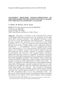
utilization of experimental Dynamic Substructuring (DS). Indeed, as the bodywork properties cannot be determined with numerical methods, its properties will have to be determined by experiments. As they are commonly measured in FRF format, the Frequency Based Substructuring (FBS) method is the preferred DS method in this thesis work. Many difficulties in this experimental DS application will have to be overcome though, because previous research showed the approach not to be accurate up to the gear noise relevant frequency of 1000 Hz [95]. Within this thesis work, several solutions were therefore developed. After each research topic is analyzed separately, all methods will be combined in an attempt to analyze the propagation of gear noise into the vehicle with enhanced accuracy. The relation between all issues with their input and output quantities is shown in figure 1. Notice that the GNP method plays a central role, as the FBS method can supply the total systems FRFs based on subsystems and the OSI method the system’s structural dynamics in operation. However, the later two methods by themselves also serve as analysis tools, which can give valuable insight in complex system behavior. Structural Dynamics GNP Method

Response

Excitations

Component Model

Assembled Model

Operational Model

FBS Method

Operational ID

Operational Parameter

Operational Model

Component Excitation Response

Figure 1: Schematic representation of issues tackled in this thesis and their relations.

Personal Contributions The major purpose of this research is to develop methods which enable the analysis of gear noise propagation in a vehicle, based on gearbox test bench measurements and the knowledge of the (operational) component system dynamics. The proposed developments of the research reported in this thesis are: • The Gear Noise Propagation (GNP) Method, which identifies a component’s operational excitation on a test bench and calculates the total system’s response to that excitation. 9

• The Operational System Identification (OSI) procedure, which enables one to measure the receptance FRF matrix elements of a stationary operating system. • A general framework for Dynamic Substructuring (DS), which simplifies the formulation of the existing experimental Frequency Based Substructuring (FBS) methods developed over the past decades. • An enhanced drivingpoint measurement method, which utilizes a 3D force sensor, to truly decouple the drivingpoint measurement in its global orthogonal x,y and z components. The experimental solution is such, that one can determine interface FRF data of subsystems at a single nodal point. • A method, which can be used to couple experimental subsystems with line and surface coupling interfaces, instead of point connections used in the past. With this technique, Rotational Degrees of Freedom (RDoF) at the subsystem interface are therefore implicitly taken into account. A filtration technique is also developed to filter the measured interface flexibilities for the best surface coupling description. • A method to determine the accuracy of the predicted DS calculation due to measurement errors made in the measurement of the subsystems. • All calculations carried out within this thesis were performed using a dedicated Matlab Toolbox. This GUI based program was developed in cooperation with BMW. All graphs presented in this work originate from this toolbox.

Thesis Outline This thesis tackles three main issues as written in the previous section. The manuscript is subsequently divided into three parts, with an additional part which combines all issues.

10

• In part I the Gear Noise Propagation (GNP) method is outlined. Chapter 1 defines the general solution which was developed. A validation of the method can be found in chapter 2. • Part II introduces a new identification method for operational systems. Chapter 3 introduces the Operational System Identification (OSI) method, which is thereafter applied on an operating vehicle tested on a dynamometer. Note that it turns out that the operational identification shows not to be required in this thesis’ vehicle application. • Part III is dedicated to the further development of today’s FBS method for the effective analysis of complex structures in higher frequencies. In chapter 5, the FBS method is placed in a general framework. Also some of the problems in experimental FBS are discussed for which various solutions are presented in chapter 6. These solutions are thereafter validated in chapter 7 on the rear axle of a vehicle.

• All developed methods are combined in part IV, chapter 8. Here, the gear noise propagation of a vehicles rear axle differential up to the driver’s ear is analyzed with combinations of the methods presented in the first three parts. Worthwhile noting is that this thesis only discusses the crucial points and results, whereas all details can be found in the publications [10, 26–37, 87, 113, 114, 116, 117] to which reference is made in the text. In summary, figure 2 shows the structure of all chapters in this thesis.

11

Introduction

PART I

PART II

PART III

GNP Method

OSI Method

DS Theory

Ch. 1

Ch. 3

Ch. 5

Validation

Validation

Methods in DS

Ch. 2

Ch. 4

Ch. 6

Validation Ch. 7

PART IV

12

Combination Ch. 8

Conclusion Ch. 9

Figure 2: Thesis outline in schematic representation.

Part I

From Test Bench to System Response Estimates

Gear Noise Identification & Propagation In part I the Gear Noise Propagation (GNP) method is outlined and validated by an experiment. With this method one can calculate the gear noise propagation of an operational gearbox into a vehicle’s bodywork. The proposed method results in physically correct responses for linear systems which are connected to the gearbox. The method consists in a gearbox measurement on a test bench and the measurement of the total system. A compensation method is outlined in case the test bench influences the measurement due to its own flexibility. In addition an extension to the method is proposed, in case one can not measure the total systems FRFs at the gearbox interfaces due to, for example, lack of space. Properties of a vehicle and gear noise excitation are nonlinearly dependent on various operational parameters. Therefore an extension to the GNP method is suggested taking into account these operational parameters. The content in this part is mainly based on our publication [30].

13

14

Chapter 1

The Gear Noise Propagation Method As stated in the introduction of this thesis, the sound level inside the car is dominated by wind noise and vibrations which are transferred from the driveline to the bodywork.1 Typical driveline excitation sources are the engine, the wheels and gears in the gearbox. Due to the ever increasing demands from customers with respect to comfort, car manufacturers seek new methods to respond to these increasing expectations. However, a further increase of acoustic comfort becomes more and more challenging since significant improvements have already been achieved based on the experience gained over the many years of car development. Furthermore, due to a massive reduction of dominant vibration sources, such as aerodynamic noise and engine excitations, new sources difficult to dominate like gear noise get into play. These vibrations are generally smaller than the total sound level, but due to their tonal character2 , they can still be experienced as disturbing. For several reasons, determination of gear noise excitations is not trivial. First of all, gear noise is nonlinearly related to several parameters, such as rotational speed, applied torque and oil temperature. These parameters are difficult to predict in advance. Secondly, the manufacturing process of the gears has a dominant influence on the actual functioning of the gearbox. This can result in a spread of the gear noise excitation level of gearboxes after production. In general, one is not able to accurately predict the level of gear noise based on theoretical models. Gear noise measurements on a test setup are therefore necessary. On such a test setup, the gearbox is typically separated from the car and mounted directly, or with rubber mountings, to a test bench (more details are found on the poster at the end of the manuscript). This allows to accurately measure the gearbox excitation forces at the test bench/gearbox interface together with various accelerations. As these responses are measured in operation, the nonlinear behavior of the gear excitation becomes apparent. It is difficult however, to translate these forces and/or accelerations to the resulting sound level 1

More information on the vehicles driveline and details on gear excitation can be found on the poster at the end of the thesis. 2 Tonal sound is also known as a periodic or harmonic sound.

15

I CHAPTER 1. THE GEAR NOISE PROPAGATION METHOD

inside the car. Different approaches exist [89, 90], but they are either physically incorrect or influenced by the test bench dynamics. In this chapter a Gear Noise Propagation (GNP) methodology, which determines the gear noise level inside the car, is outlined. Gear noise measurements on a test setup are used, as well as a measurement of the entire vehicle’s FRFs. As such, the GNP method can be seen as a special class of the well known TPA analysis. Section 1.1 introduces the theoretical development of the method. Section 1.2 presents a compensation method for test bench influences. A different measurement strategy for nonmeasurable interfaces is presented in section 1.3. This chapter proceeds with an extension to the GNP method, describing how one can linearize the operating system excitation about an operating point, as well as a comparison of the GNP method with the classical approach in TPA by placing the latter method in the GNP framework, in sections 1.4 and 1.5. This chapter ends with a summary in section 1.6. The validation of the presented method can be found in chapter 2.

1.1

Theory

Gear noise is a combination of the harmonic excitation generated by the contact forces between gears and the noise generated by bearings inside the gearbox.3 It is impossible to measure these excitation forces, as the gears are rotating during operation. One can therefore not determine the true gear noise excitation forces themselves (see figure 1.1.a). The following derivation shows that instead of the true gear noise excitation forces, a different set of excitation forces can be defined, which equivalently represent the gear noise excitation force. Proposed equivalent set of forces can be utilized to calculate the physically exact gear noise propagation in the total structure.4 This method carries the name Gear Noise Propagation (GNP) method and holds for linear, time invariant structures in stationary operation. A discussion on how to include nonlinear structures can be found in section 1.4. Figure 1.1.b demonstrates its working principle, schematically explaining the propagation of gear noise to the systems in front of the gearbox.5 The GNP method is best explained by using the simplified gear noise propagation model in figure 1.1.b. The model shows a gearbox driven by several shafts, applying torques M and driving speeds n . The bodywork structure is excited by the resulting unknown gear noise force fgear or equivalent forces fequivalent , yielding structural responses u and sound pressures p . First, imagine a gearbox (gb) attached to the bodywork (bw) of a vehicle that is driven during operation by shafts, applied torques M and driving speeds n . The operating

16

3

In this thesis a vehicle’s Rear Axle Differential (RAD) is analyzed as shown in the poster at the end of this thesis. As such, the denotation “gearbox” refers to this type of gearbox. Notice however that the presented theory is applicable to any kind of structural component which excites the total structure through well defined coupling interfaces. 4 Notice that the nonlinear relation of the gear excitation towards torque, rotating speed and oil temperature, is indirectly included in the equivalent forces, if they are measured on the test bench in the corresponding operational states. 5 By “in front of the gearbox” all those subsystems are meant that are connected to the gearbox, from which the noise originates.

I

1.1. THEORY

p3

p3

u3

u3

(bw)

u2

u1

fgear = ?

(gb)

M2 , n 2

(bw) u2

u2

u2

fequivalent

(gb)

M1 , n 1 (a)

u2 fequivalent u2

(b)

Figure 1.1:

Schematic representation of the gear noise propagation method for a gearbox (gb) and bodywork (bw) assembly with: (a) the unidentifiable gear noise excitation force between the gears and (b) the implementation of measured test bench forces to calculate responses inside the vehicle.

gearbox will then excite the system by nonmeasurable gear noise forces (fgear ) between the gears (figure 1.2.a). The partitioned Equations of Motion (EoM) of the total system (gearbox and bodywork) can be written in the frequency domain using a dynamic stiffness representation:6 ⎡ ⎤(tot) ⎡ ⎤ ⎤ fgear Z11 Z12 0 u1 ⎣ Z21 Z22 Z23 ⎦ ⎣ u2 ⎦ = ⎣ 0 ⎦ , 0 Z32 Z33 u3 0 ⎡

(1.1)

where Zij represent the dynamic stiffness matrix pertaining to the partition ij, and where [u1 u2 u3 ]T denote the displacements respectively at the gears contact surface, the gearbox interface to the bodywork and positions of interest on the bodywork. The gear contact surface is also referred to as gear face7 and interesting positions on the bodywork (u3 ) could, for example, be the interface to the driveline or any other physical property like the sound level at the driver’s ear. In the latter case, the displacements u3 is interchanged by p and the FRFs of the bodywork now have different units, depending on their inputoutput relation. In (1.1) the (tot) superscript denotes the total system (gearbox plus bodywork). Since the gearbox and the bodywork have only degrees of freedom u2 in

6 7

See appendix 8.4 for a derivation and illustration on the used symbolics. See appendix 8.4 for more details on gear topology.

17

I

p3 u3

fgear

u2

CHAPTER 1. THE GEAR NOISE PROPAGATION METHOD

u2 = 0

(bw) u1

fgear

(gb) (gb)

u2 = 0

u2

(a)

(b)

p3

fequivalent

uequi 3

fgear

u2 = 0

(bw)

ufi 1

fequivalent u2 = 0

uequi 2

uequi 2 fequivalent

uequi 2

uequi 1

fequivalent (gb)

(c)

(d)

18

Figure 1.2: Overcoming the problem of unmeasurable gear noise excitation between the gears (fgear ), with simplified models of: (a) real problem, (b) internally generated gear noise, (c) freebody diagram of the gearbox constrained to the fixed world and (d) implementing the identified gear noise interface forces (fequivalent ) in the GNP method. Notice that a 3 DoF system is suggested in this figure. However, the method is applicable for any number of DoF. common one can also write: ⎤ ⎤(tot) ⎡ (gb) (gb) Z12 0 Z11 Z11 Z12 0 ⎢ (gb) (tot) (bw) ⎥ ⎣ Z21 Z22 Z23 ⎦ = ⎣ Z21 Z22 Z23 ⎦ (bw) (bw) 0 Z32 Z33 0 Z32 Z33 ⎡

(1.2)

I

1.1. THEORY

where indices (gb) and (bw) denote the gearbox and bodywork respectively and where (tot)

Z22

(gb)

(bw)

= Z22 + Z22 ,

(1.3)

is the dynamic impedance assembled on the interface. Hence it is understood that Z11 , Z12 , Z21 always pertain to the gearbox and Z33 , Z32 , Z23 always pertain to the structure in front of the gearbox (the bodywork in the present case). Hence the superscript for those submatrices will be dropped and it will only be indicated for the Z22 if it corresponds to the total system or to one of the subsystems. Also notice that, in this research, the gearbox is actually attached to the test bench with its rubber mountings.8 This means that the properties of the mountings are included in the description of the gearbox prop(gb) erties, i.e. Z11 , Z12 , Z21 and Z22 . In the remaining text reference is only made to the gearbox for the reason of simplicity though. Condensing equation (1.1) on the interface (u2 ) yields 



 (tot) −1 −1 u2 fgear −Z21 Z11 Z22 − Z21 Z11 Z12 Z23 = . (1.4) u3 0 Z32 Z33

Equation (1.4) represents the response of the vehicle’s bodywork (u2 , u3 ) due to the gear noise excitation between the gears (fgear ). So far the result of equation (1.4) is of little use, as one is not able to measure the gear noise excitation force (fgear ). However, let us now assume that the gearbox is measured separately on a rigid test bench (fixed boundary) as shown in figure 1.2.b. The EoM of this setup is equal to 

 

Z11 Z12 fgear uf1 i , (1.5) = (gb) finterf ace 0 Z21 Z22 where the superscript f i in uf1 i indicates that this solution corresponds to the fixed interface experiment described in figure 1.2.b (for which figure 1.2.c is the free-body diagram). A fundamental assumption implicitly used here, is that the gear forces (fgear ) exciting the system are independent of the total system’s global dynamics. Obviously this in not exactly the reality. Nevertheless, the harmonic excitation will probably not deviate between both configurations much if the gearbox is decoupled from its environment with the same rubber bushings and excited with the same torque, gear rotation speed and oil temperature in both configurations. This is due to the construction of most gearboxes. A gearbox has a very stiff housing and therefore does not experience large dynamic deformation if it is decoupled from its environment with soft rubber bushings. Consequently, the deformation of the gear faces, bearings and gear axis as well as the gear lubrication mainly determine the harmonic gear noise excitation. Also, note that the responses of the gearbox are not the same for both setups, i.e. the gearbox vibrates differently on the test bench and the total vehicle. This is denoted in equation (1.5) as uf1 i . A more detailed discussion is found in section 1.4.

8

See the poster at the end of the thesis.

19

I

Figure 1.2.c is the free body diagram of the gearbox in figure 1.2.b, where the interface force between the gearbox and the test bench are such that u2 = 0. This interface force is denoted fequivalent for later purposes, i.e.: 

 

Z11 Z12 fgear uf1 i , (1.6) = (gb) fequivalent 0 Z21 Z22

CHAPTER 1. THE GEAR NOISE PROPAGATION METHOD

where

20

fequivalent = finterf ace .

(1.7)

Eliminating uf i in (1.6) leads to −1 fgear . fequivalent = Z21 uf1 i = Z21 Z11

(1.8)

The equation shows that there is a direct relation between the unknown gear forces (fgear ) and the interface force of the gearbox to the rigid test bench (fequivalent ). It is only dependent on the properties of the gearbox. Now imagine the following situation: the interface force (fequivalent ) between the gearbox and the rigid test setup is applied as an external excitation at the gearbox/bodywork interface (see figure 1.2.d). The associated EoM are ⎤ ⎡ ⎤ ⎡ equi ⎤ ⎡ Z11 Z12 0 u1 0 equi ⎥ ⎣ Z21 Z (tot) Z23 ⎦ ⎢ (1.9) ⎣ u2 ⎦ = ⎣ −fequivalent ⎦ . 22 equi 0 0 Z32 Z33 u3 where the notation uequi is used to indicate that the displacements obtained at this stage are obtained by applying the force fequivalent as external force on the interface (figure 1.2.d). At first glance, equations (1.1) describing the real situation where the system is excited by the gear noise and (1.9) seem different. However, a condensation of equation (1.9) on the gearbox interface yields   

equi (tot) −1 u −fequivalent Z22 − Z21 Z11 Z12 Z23 2 = 0 uequi Z32 Z33 3

 −1 −Z21 Z11 fgear = , (1.10) 0 This last result is identical to equation (1.4) which shows that the response on the bodywork (u2 , u3 ) to the gear noise excitation can be obtained equivalently by solving the problem of figure 1.2.d, namely when fequivalent is applied as external force on the interface. This proves that the problems depicted in figure 1.2.a and in figure 1.2.d are exactly equivalent for what concerns the response in front of the gearbox. However, comparing : the responses computed inside the gear(1.1) and (1.10) it is obvious that u1 = uequi 1 box by the equivalent problem are different from the actual internal gearbox responses. This is however not an issue since one is only interested in predicting the response of the subsystems in front of the gearbox in practice. In summary:

I

1.1. THEORY

The response of subsystems in front of the gearbox (including the degrees of freedom on the interface) can be equivalently computed by applying at the interface the force fequivalent produced by the gearbox on a rigid test bench. The response inside the gearbox will however be different.

This result shows that the actual source of the gear noise excitation (fgear ) does not need to be directly measured. It is sufficient to measure equivalent forces at the gearbox interface to the fixed world. The equations are written in the dynamic stiffness format. This was very useful in the derivation performed, due to the zero off-diagonal terms Z13 and Z31 indicating that there is no direct structural coupling between the inside of the gearbox and the inside of the bodywork. Unfortunately, in most real applications, it is however impossible to measure dynamic stiffness since it requires imposing displacements and measuring reaction forces. Equation (1.9) is therefore transformed into the receptance formulation. Premultiplying (1.9) by the inverse of the impedance (namely the receptance matrix Y of the total system) results in:9 ⎤ ⎡ equi ⎤ ⎤(tot) ⎡ Y11 Y12 Y13 0 u1 ⎣ Y21 Y22 Y23 ⎦ ⎣ −fequivalent ⎦ = ⎣ u2 ⎦ , Y31 Y32 Y33 0 u3 ⎡

(1.11)

Considering now only the last set of equations in (1.11) yields the simple relation for the responses at and in front of the gearbox interface

u2 u3



= −

Y22 Y32

(tot)

fequivalent .

(1.12)

The above result shows once more that the internally generated gear forces are not required to determine the gear noise responses in the total system. The correct result is obtained by applying at the connections of the total system the forces delivered by the operating gearbox to the fixed world. In practice, the method boils down to measuring the gearbox interface forces on a rigid test bench, and measuring the receptance of the total system for the gearbox connection and for the outputs of interest in/on the bodywork. The latter could also be calculated using a FEM model and/or a experimental Frequency Based Substructuring (FBS) method [20, 29, 66]. These calculations would enable optimizing structural components for the given excitation. The test bench measurement is performed with different operating conditions, to determine the operational dependency of the gear excitation. As stated at the beginning of this section, the method is based on linearity of the subsystems. This contradicts the nonlinear relationship of, for example, the various rubber mountings and the large static deformation introduced by the engines applied torque during operation. A discussion on such nonlinearities and the implications on the theory can be found in section 1.4.

9

See appendix 8.4, i.e. Y = Z −1 .

21

I 1.2

Compensation for Nonrigid Test Benches

CHAPTER 1. THE GEAR NOISE PROPAGATION METHOD

A test bench will probably not be rigid in the mid frequency range (100-1000Hz) where gear noise is analyzed. Rigidness is, however, a requirement of the Gear Noise Propagation (GNP) method as introduced in the previous section. In this section, the GNP method is extended for the case of a flexible test bench. Here we concentrate on finding the equivalent force (fequivalent ) defined in (1.6) for a measurement on a flexible test bench. In this way physically correct responses at and in front of the gearbox interface can be determined according to the theory described in the previous section. In order to clarify the mathematical elimination of test bench flexibilities, assume the gearbox is operating on the flexible test bench as illustrated in figure 1.3. Again the

unrtb 3 unrtb 2

(t b)

fsensor

unrtb 3 fgear

unrtb 2

unrtb 2 unrtb 1 (gb)

fsensor unrtb 2

Figure 1.3:

A schematic drawing of a flexible test bench measurement. The flexible test bench responses will influence the measured interface forces at the gearboxes’ interface. The sensor forces at the interface therefore do not identify the equivalent forces defined in section 1.1.

22

unknown gear noise forces between the gears (fgear ) excite the system and sensors measure the interface forces (fsensor ) and displacements (u2 ) between the gearboxes’ rubber mountings and the test bench.10 Note that the interface forces are now influenced by the test bench responses and therefore do not represent the equivalent forces (fequivalent ) as required for equation (1.12), i.e. fequivalent = fsensor . The equations of motion for the system is represented by (see figure 1.3): 





 Z11 Z12 0 unrtb fgear 1 + = (1.13) (gb) fsensor 0 unrtb Z21 Z22 2

10

See the poster for an illustration.

I

1.2. COMPENSATION FOR NONRIGID TEST BENCHES



(tb)

Z22 Z32

Z23 Z33



unrtb 2 unrtb 3



=

−fsensor 0

 ,

(1.14)

where u3 represents as before the degrees of freedom outside of the gearbox (here, the test bench) and where the superscript nrtb indicates that the responses are obtained on a non-rigid test bench. The superscript (gb) and (tb) denote the gearbox and test bench. By condensation of equation (1.13) on the interface between the gearbox and the test bench, one obtains:

(gb) −1 −1 Z22 − Z21 Z11 Z12 unrtb = −Z21 Z11 fgear + fsensor , (1.15) 2 which, taking account of (1.8), reduces to

(gb) −1 Z22 − Z21 Z11 Z12 unrtb = fsensor − fequivalent . 2

(1.16)

= 0 one finds the definition of fequivalent in (1.7) as the Clearly this shows that if unrtb 2 interface force measured by the sensor on the perfectly rigid world. In the present case, however, the test bench experiences a dynamic response, which introduces displacements on the interface, i.e. u2 = 0, and by which the sensor force (fsensor ) is different from the equivalent force (fequivalent ). If the connecting forces fsensor and the displacements u2 are measured during the test, equation (1.16) allows reconstructing the required equivalent force fequivalent . The equation shows that it is not necessary to know the dynamic stiffness of the test bench, but it is the knowledge of the gearboxes’ dynamic properties which is required. A further simplification of equation (1.16) is possible. First, let us rewrite (1.16) in the equivalent form 



 Z11 Z12 u1 0 = . (1.17) (gb) fsensor − fequivalent unrtb Z21 Z22 2 where the notation u1 is used to indicate that in this equation the gearbox response is not in (1.13). By transforming the equation above into the receptance matrix equal to unrtb 1 representation of the gearbox, one obtains

Y11 Y12 Y21 Y22

(gb)

0 fsensor − fequivalent



=

u1 unrtb 2

 .

(1.18)

The second line of this result yields (gb)

Y22

(fsensor − fequivalent ) = unrtb , 2

(1.19)

(gb)

where Y22 is the receptance of the gearbox as seen from its connection degrees of freedom. Finally, inverting this relation, one finds (gb)

fequivalent = fsensor − Z22

unrtb , 2

(1.20) 23

I

(gb)

(gb)

CHAPTER 1. THE GEAR NOISE PROPAGATION METHOD

where Z22 is the inverse of Y22 and thus represents the dynamic stiffness of the gearbox as seen from its connection. Comparing (1.20) to (1.16) it is clear that

24

(gb)

Z22

(gb)

−1 = Z22 − Z21 Z11 Z12 ,

(1.21)

representing the dynamic stiffness of the gearbox condensed on the connection degrees of freedom. Physically it corresponds to the gearbox dynamic stiffness seen at the interface when the degrees of freedom u1 internal to the gearbox are free. Equations (1.19) and (1.20) clearly show that one can compensate for test bench dynamic influences on the measured gear noise using the gearbox interface flexibility or stiffness. No system properties between the gears and the gearbox’s interfaces are needed, nor properties of the test bench itself. The receptance matrix of the gearbox interfaces can be obtained by either a modal analysis of the freely suspended gear box, a direct FRF measurement of the gearbox, or by a FEM calculation. To summarize, the Gear Noise Propagation method of section 1.1 can be applied even when the test bench used to measure fequivalent is not fully rigid. In that case equation (1.19) or (1.20) should be used. This involves in practice that, when measuring the gear noise excitation, additional accelerometers at the gearbox interface points are required in (see figure 1.3 and the poster). Furthermore, the gearbox receptance order to measure unrtb 2 (gb) matrix Y22 is needed. The determination of this receptance matrix is discussed in chapter 2.

1.3

The GNP Method Extended for Nonmeasurable Interface FRFs

Nowadays, gearboxes are embedded into the total system in a very compact way. This means that in practice one might not be able to access all the gearbox interface nodes in the total system configuration with an impulse hammer or shaker. For instance when a gearbox is mounted under the body of a car the places where it is connected to the rest of the car can barely be accessed. Hence measuring the receptance (tot) (tot) Y22 and Y32 needed in the GNP procedure (see equation (1.12)) might not be feasible due to the lack of space around the interface nodes which prohibits connecting shakers or apply an impulse by hammer. In such cases, the GNP method can no longer be applied and a different solution is needed. The method proposed in this section is in fact an extension of the GNP discussed so far. In the GNP theory described in section 1.1 an equivalent force was applied at the connection degrees of freedom such that the dynamic response in front of the gearbox is identical to the response obtained with the actual gear noise. Here that idea is generalized by searching an equivalent force (called substitute force fsubs ) such that, when applied on degrees of freedom on points anywhere on the gearbox (called substitute nodes), it creates a dynamic response in front of the gearbox identical to the response that would be obtained with the true gear noise. This concept is schematically explained in figure 1.4. In figure 1.4.a the original gear noise problem is depicted. Figure 1.4.b represents the equivalent problem as discussed in section 1.1 and figure 1.4.c corresponds to the situation

I u2

1.3. THE GNP METHOD EXTENDED FOR NONMEASURABLE INTERFACE FRFS

p3 u3

(bw) u1

fgear

(gb)

p3

(bw)

(a)

uequi 2

p3

usubs 3 (bw)

usubs 2

usubs 4

uequi 3

u2

uequi 2

fequivalent

uequi 2

uequi 1

fequivalent (gb)

uequi 2

(b) (gb)

usubs 2

fsubs

(c)

Figure 1.4:

Overview of the different forces and DoF sets to explain the replacement of the equivalent forces by the substitute forces: (a) the original problem with an nonmeasurable gear noise excitation force fgear , (b) the equivalent problem with the equivalent forces fequivalent that can be measured on a rigid test bench as described in section 1.1 and (c) the substitute problem with the virtual substitute force fsubstitute applied on nodes for which the dynamic admittance can be measured in practice.

considered here, assuming that the substitute nodes are nodes that can be easily accessed and thus for which the dynamic receptance can be easily measured in the total system. It will now be shown how the substitute force fsubs can be determined, such that its response obtained in front of the gear box are identical to the original gear noise problem. It was shown in section 1.1 that the equivalent problem of figure 1.4.b is described by equations (1.12) with the equivalent force fequivalent obtained from (1.8). If the gearbox 25

I

system is now considered through its interface degrees of freedom u2 and substitute degrees of freedom u4 , the EoM of the problem described in figure 1.4.c writes ⎡ ⎤ ⎤ ⎡ subs ⎤ ⎡ 0 Z44 Z42 fsubs u4 ⎦ = ⎣ 0 ⎦, ⎣ Z24 Z (tot) Z23 ⎦ ⎣ usubs (1.22) 2 22 subs 0 u3 0 Z32 Z33

CHAPTER 1. THE GEAR NOISE PROPAGATION METHOD

where the superscript subs is introduced to indicate that the responses correspond to the situation described in figure 1.4.c. Note that in these equations the degrees of freedom u1 are not considered.11 Condensing equation (1.22) to eliminate the substitute degrees of freedom u4 , one finds

 

 (tot) −1 −1 usubs fsubs −Z24 Z44 Z22 − Z24 Z44 Z42 Z23 2 = , (1.23) usubs 0 Z32 Z33 3 or in a reduced receptance matrix representation (also see section 1.1): 

(tot)

  Y22 u2 −1 = −Z24 Z44 fsubs . u3 Y32

(1.24)

If the responses of this problem are then requested to be identical to the responses [u2 u3 ]T of the original gear noise problem, and thus to the responses obtained from the equivalent problem described by (1.12), one finds



 (tot)   Y22 0 −1 = . (1.25) Z24 Z44 fsubs − fequivalent Y32 0 This holds for all frequencies if and only if −1 Z24 Z44 fsubs = fequivalent .

(1.26)

Hence an equivalent substitute force can be found if a solution fsubs can be computed −1 from (1.26) for any fequivalent . This is the case if Z24 Z44 defines a non-overdetermined −1 T problem, e.g. if and only if the nullspace of (Z24 Z44 ) is empty. namely if the rank of −1 is smaller or equal to the dimension of u2 . In practice it means that one needs −Z24 Z44 at least as many substitute degrees of freedom u4 as connections degrees of freedom u2 . The substitute force can also be computed using fequivalent (measured on a test bench) and measured receptances of the gearbox. Indeed note that, if the receptance of the gearbox is known for the substitute and interface nodes, one can write (gb)  (gb)

Y22 Y24 Z24 Z22 = I. (1.27) Y42 Y44 Z42 Z44

26

11

It should also be noted that the dynamic stiffness matrices of the gearbox considered in (1.22) are different from those considered in section 1.1. For instance, it is implicitly assumed here that the dynamic stiffness is obtained when all DoF different from u2 and u4 are free, whereas in the previous section it was assumed that (tot) (gb) (bw) all DoF are free except u1 and u2 . This implies for instance that in equation (1.22), Z22 = Z22 + Z22 (gb) (gb) is as in (1.3), but now Z22 is a different matrix, since the matrix Z considered here pertains to the degrees of freedom u2 and u4 .

I

1.3. THE GNP METHOD EXTENDED FOR NONMEASURABLE INTERFACE FRFS

From (1.27) one finds (gb)

(gb)

(gb)

(gb)

Y22 Z24 + Y24 Z44 = 0 Y42 Z24 + Y44 Z44 = I,

which, after development, leads to the relations (gb)

(gb)

(gb)

(gb)

(gb)

(gb)

− Y42 (Y22 )−1 Y24 ]−1

Z44 = [Y44

(gb)−1

Z24 = −Y22

Y24 [Y44

(gb)

(gb)

(1.28) (gb)

− Y42 (Y22 )−1 Y24 ]−1 .

(1.29)

Substituting in (1.26) one finds: −1 + ) fequivalent fsubs = (Z24 Z44 (gb)−1

= −(Y22

(gb)+

= −Y24

(gb)

Y24 )+ fequivalent (gb)

Y22 fequivalent ,

(1.30)

Since there might be more DoF in u4 than u2 , Y24 might be non-square and in that case (gb)+ represents the pseudo-inverse of Y24 . Y24 In summary it was shown that one can compute a force fsubs such that the equations (1.22) yield the same dynamic response in front of the gearbox as for the original problem. In practice, inverting (1.22), the responses would be computed using the receptances of the total system as follows:

u2 u3



=

Y24 Y34

(tot)

fsubs ,

(1.31)

To conclude, the above result has shown that substitute nodes on the gearbox may be used to determine the gear noise propagation into the total system. Physically exact results are obtained for the responses at and in front of the gearbox interface. This modified GNP procedure includes thus the following steps: • measure the equivalent gear forces (fequivalent ) on a rigid test bench or with compensation for its flexibility (section 1.2) ;

• measure the total systems FRFs from the substitute nodes to interesting points at and in front of the gearbox interface. ; • Obtain the FRFs for the

gearbox alone

at the substitute nodes and the gearbox (gb) (gb) interface, namely Y42 and Y22 (by testing or simulation) ; • compute the substitute force fsubs satisfying (1.26), by applying equation (1.30) ; • compute the response to the gear noise using (1.31). 27

I 1.4

Including Operational Parameters & Nonlinearities in the GNP Method

Up to now, only linear systems were considered in the presented GNP method. In addition, little attention was given to the operational (and nonlinear) behavior of the gear noise excitation. This section discusses the implications of, and the possibility to include, different kinds of operational parameter and nonlinearity. In this thesis the following kind of operational parameter and nonlinearities are believed to be dominant and will therefore be discussed:

CHAPTER 1. THE GEAR NOISE PROPAGATION METHOD

• The dependency of the gear noise excitation on rotating speed (n), applied torque (M ), oil temperature (T ) and the global (quasi-static and dynamic) motion of its housing. • The dependency of the rubber mountings on large deformations and the viscoelastic material behavior of the rubber depending on temperature. • The dependency of the remaining vehicle components on driving speed, applied torque and temperature, i.e. the drive shaft and the car interior.

As the gear noise, produced by the gearbox, is measured on the test bench in operation, the (nonlinear) dependence of the gear excitation on the operational parameters will be implicitly measured. Since the rubber mountings are included in the measurement, their nonlinear response on the operational parameters will also be part of the measurement. It is therefore possible, assuming the vibrations to remain small, to write equation (1.12) as the acoustical response inside the vehicle by a linearisation of the operational parameters in their stationary operating condition, i.e.



(tot) u2 (jω, n, M, T ) Y22 (jω) =− fequivalent (jω, n, M, T ). (1.32) u3 (jω, n, M, T ) Y32 (jω)

Notice however, that this approach is only valid, in case the real gear noise force fgear is the same for the test bench and vehicle configuration. In chapter 2 the assumption of the gear noise excitation independency with respect to the total system’s dynamics will be validated. In that chapter, one can also find more details on the dynamic mechanisms that (could) affect the gear noise excitation. Let’s for now assume that the GNP approach holds. In that case, the (nonlinear) functional given by equation (1.32) only includes the operational parameters of the gearbox excitation and its mountings. The remaining vehicle parts, however, are believed to depend on the operating parameters as well.12 It is believed that their relation is nonlinear in nature also. As the total system’s properties change in operation, an erroneous outcome from the GNP method can therefore be expected. This calls for an operational identification of the total vehicle’s dynamics13 , such that the GNP method can be extended with

28

12

The vehicle properties were considered unaffected by operation up to this point and should be determined by standard FRF measurement. 13 In Part II of this thesis, chapter 3, the operational system identification is subject of research.

I

1.5. COMPARISON WITH THE TRANSFER PATH ANALYSIS (TPA) METHOD

linearized operational vehicle properties as well, e.g.:

u2 (jω, n, M, T ) u3 (jω, n, M, T )



=−

Y22 (jω, n, M, T ) Y32 (jω, n, M, T )

(tot)

fequivalent (jω, n, M, T )

(1.33)

For this equation to hold, it is essential that the structural dynamics of the gearbox and the (gb) rubber mountings (Z11 , Z12 , Z21 and Z22 ) are the same in the total vehicle and the test bench configuration. As the same driving speed, torque and temperature are simulated on the test bench, this will probably be a good assumption. Specific details on the differences can be found in chapter 2.

1.5

Comparison with the Transfer Path Analysis (TPA) Method

The classical approach in TPA analysis [90] can also be placed in the GNP framework derived in the previous sections. To do so, consider the EoM of the total vehicle separated at the gearbox interface, as shown in figure 1.5: 



(tot)

 Z11 Z12 0 u1 fgear + = (1.34) (gb) u2 0 finterface Z21 Z22 

(bw)

Z22 Z32

Z23 Z33



u2 u3



(tot) =

−finterface fother

 .

(1.35)

(tot)

are internal nodes of the vehicle, which might also be excited Here, displacements u3 by other (driveline) forces contained in fother . In classical TPA approaches, the interface forces finterface are measured in the operating vehicle configuration by built-in force sensors, or alternatively these interface forces are determined from acceleration measurements.14 The classical TPA approach thereafter uses the (operational) interface forces by combining them with the free bodywork properties, determining the sound pressure at the driver’s ear. Indeed, inversion of equation (1.35) yields

Y22 Y23 Y32 Y33 (tot)

→ u3

(bw)

−finterface fother (bw)

= −Y32



 =

(tot)

u2 (tot) u3

(bw)

finterface + Y33



fother ,

(1.36)

which means that the responses at for example the driver’s ear can be determined, in a physically exact way, if the gearbox interface forces finterface and the other driveline forces fother are known. From a theoretical point of view, the classical TPA and GNP method

14

The acceleration based methods are commonly known as the mounting stiffness method [91] and the matrix inverse method [91]. Both methods basically combine the measured accelerations with stiffness properties to determine the interface forces.

29

CHAPTER 1. THE GEAR NOISE PROPAGATION METHOD

I

p3 u3 fother

u3 (bw)

u2 finterface

fgear

u2

u2

u1

finterface (gb)

u2

Figure 1.5:

Overview used for a comparison of the classical TPA and the GNP method. Here the nonmeasurable gear noise excitation force is denoted fgear , some other excitation sources are denoted fother and the interface forces between the gearbox and the bodywork is denoted finterf ace . Note that the total vehicle denoted (tot) in equations (1.34) through (1.38) is the assembly of the gearbox (gb) and and bodywork (bw) subsystems.

therefore only differ in their approach, yielding the same sound pressure contributions at the driver’s ear.15 However, a disadvantage of the classical TPA method, compared to the GNP method, is that the interface forces are not only dependent on the excitation of the gearbox. They are also dependent on the displacement at the gearbox’s interface. This displacement results from all vehicle excitations. Indeed analog to equation (1.16) one finds from (1.34) the interface forces as

30

finterface

=

(gb) (tot) −1 −1 Z22 − Z21 Z11 Z12 u2 + Z21 Z11 fgear (gb)−1

= Y22

(tot)

u2

−1 + Z21 Z11 fgear .

(1.37)

This implies that structural optimizations of the driveline and / or the vehicle bodywork, as well as changes in the other excitations fother will influence the interface forces. Indeed, combining equation (1.34) and (1.35) and inverting the result, shows the interface displacements are dependent on

15

Notice that the presented GNP and TPA approaches not only hold for gearboxes, but also for the engine and other driveline parts.

I

1.5. COMPARISON WITH THE TRANSFER PATH ANALYSIS (TPA) METHOD

(tot)

u2

(tot)

= Y21

(tot)

fgear + Y23

fother ,

(1.38)

which means that the vehicle components and the gearbox excitation can not be optimized separately, complicating the optimization process. Changes to the gearbox excitation, the other (driveline) excitations as well as changes to the vehicle properties, all require a renewed measurement of the interface forces in the total vehicle configuration. To conclude the comparison of the TPA and GNP method one can make the following observations: • The GNP method is based on equivalent forces which are independent of the test bench and the vehicle bodywork properties. This is not the case for the TPA method, as the interface forces used are always dependent on the total vehicle configuration or test bench. Compared to the TPA method, the GNP method therefore allows to tune the driveline component excitations on the component test bench with respect to the response in the total vehicle, without performing a new vehicle measurement. • The TPA analysis is usually combined with a measurement of the gearbox on a test bench as discussed in section 1.2. The determination of the interface forces on the test bench are now clearly dependent on the test bench stiffness though, as the properties of the bodywork in (1.35) are replaced by the stiffness of the test bench.16 If the dynamic stiffness is not the same as the one from the vehicle’s bodywork, an error on the interface forces estimate will be made. This means that in reality a classical TPA synthesis with measured interface forces at a component test bench could yield unrealistic sound pressures at the driver’s ear. • When inserting a force sensor at the interfaces, as done in the classical TPA approach, one can influence the total vehicle properties and hence the interface forces itself. This is not the case for the GNP method. • Nonlinearities of the vehicle and its components have different effects in both methods, as they are based on measurements of different configurations. The advantage of the GNP method is that the total vehicle properties are determined in its actual configuration. However, the properties of the component on the test bench might change due to the fixation at its interfaces. One can on the other hand also question the measurement of the bodywork in the TPA method, as its properties might change with its installed driveline components as well. Especially if the component engine is analyzed, which considerably modify the vehicle due to its considerable mass, differences could get into existence. • TPA requires the bodywork properties, whereas the GNP requires the total vehicle properties (i.e. the assembled gearbox and bodywork). The GNP method therefore requires less effort for the determination of one vehicle’s FRF. However, it also implies that one vehicle with different driveline types should all be separately measured for

16

See also equation (1.13) and (1.14).

31

CHAPTER 1. THE GEAR NOISE PROPAGATION METHOD

I 32

the GNP method, whereas this is not the case for the TPA method. Depending on the amount and the differences between different driveline types, the TPA or GNP method might be more convenient to apply. Notice that one can overcome measurement of different vehicle types if the total vehicle properties are determining with dynamic substructuring, see part III.

• In cases where a vehicle’s driveline component is used in different bodywork types, which is the case for vehicle engines for example, the GNP method has an advantage over the classical TPA analysis. Indeed, in such cases the test bench stiffness would need to be changed for each different bodywork type for the TPA analysis, whereas no changes have to be made to the rigid test bench in case the GNP method is applied. • Notice that in both methods, optimizing the dynamic properties of the vehicle components, such that the structural properties of the total vehicle are significantly changed, strictly requires a renewed measurement of the vehicle FRF for the GNP method and a new measurement of the vehicle’s operational interface forces in TPA if the test bench did not exactly represent the vehicle’s interface stiffness. • It is time consuming to integrate force sensors between the gearbox and bodywork interface, necessary for the TPA analysis. It should also be noted though that determining the vehicle FRF required for the GNP method might pose difficulties. Indeed, as noted in section 1.4 interfaces might not always be accessible in modern vehicles which are built in a compact way. Removing the driveline components as done in the TPA analysis makes the interface accessible, most of the time.

1.6

Summary

In this chapter, a new paradigm to measure gear noise propagation was introduced. With this method one can calculate the gear noise propagation of an operational gearbox into a vehicle’s bodywork. The proposed method results in physically correct responses for the linear(ized) systems, which are connected to the gearbox. In order to calculate this propagation, various measurements and calculations need to be carried out. First of all, the method requires a gear noise measurement of the gearbox on a test bench. The gearbox is measured separately from the total system, e.g. without the vehicle’s bodywork. Sensors measure the interface forces (fsensor ) and displacements (u2 ) between the gearbox and the test bench. Secondly, the receptance of the total system, including the gearbox, is measured at the gearbox interface point as well. The interface receptances are measured between the (tot) (tot) interface nodes and points of particular interest in the structure, namely Y22 and Y32 . If the test bench is rigid, one can directly calculate the gear noise propagation on (tot) (tot) the knowledge of fsensor , Y22 and Y32 according to equation (1.12) with fequivalent = fsensor . In case the test bench has dynamics of its own, one has to compensate first the test bench influences in the measured forces (fsensor ). To do so, the receptance matrix

I

1.6. SUMMARY (gb)

of the gearbox at the interface nodes (Y22 ) is required. The compensation is performed using equation (1.20). In practice one might not be able to measure the interface FRFs of the total system due to space limitations. It was shown that instead of measuring these FRF, substitute FRFs measured on different positions on the gearbox may also be used. The equivalent forces fequivalent can be translated into substitute forces fsubs upon equation (1.30). Physically exact responses at and behind the gearbox interface are found. For this analysis additional knowledge of the receptance matrix elements between the substitute nodes and (gb) (gb) the interfaces are however needed, i.e. Y22 and Y24 . The responses are calculated with equation (1.31). Section 1.5 places the TPA method in the framework of the GNP method. It is shown, that in theory physically exact responses at the driver’s ear can be determined upon the knowledge of the component - bodywork operational interface forces and the receptance matrix of the bodywork subsystem. It is however shown that the interface forces are dependant on both the driveline components and the bodywork properties. As such, it is not possible to separately tune the driveline component’s excitation at a test bench, underlining the benifit of the GNP method. The flowchart shown in figure 1.6 summarizes all the important steps and equations. The dependency on the operational parameters (see section 1.4) are however omitted for the sake of simplicity.

33

I CHAPTER 1. THE GEAR NOISE PROPAGATION METHOD

Start

Start

Start

Start

Gear Noise Measurement on Test Bench

fsensor

Yes Rigid Test Bench?

fequivalent = fsensor

No fequivalent =

usensor

*

Receptance Measurement on Gearbox Interface

gb u2 fsensor - Z22

gb Y22

fequivalent

gb

Gearbox Receptance Y24 Measurement on Substitude Node

+

gb gb fsubs = Y24 Y22

Y22 Y24

fequivalent

Y32 Y34

No FRF Measurement of Total Vehicle at Gearbox Interface

tot Y2* Measurable?

Y22 Y32 Yes

tot

f2 fsubs

=

u2 u3

tot

u2 u3

tot

= -

Y22 Y32

tot

fequivalent

34

Gear Noise Propagation in Vehicle

Figure 1.6: Flowchart for the application of the GNP method.

I

Chapter 2

Measurements, Results & Validation

In this chapter the GNP method is validated on the gear noise propagation of a vehicle’s Rear Axle Differential (RAD). The goal is set to determine the sound level response at the driver’s ear according to the GNP method. For details on the vehicle’s driveline, the used abbreviations and details on gearing, the reader is referred to appendix 8.4 and the poster included at the end of this thesis. The validation made in this chapter is twofold. First it will be investigated if the gear noise excitation fgear is independent of the quasi-static deformation and global systems’ dynamics for the given framework, e.g. built on the test bench or in the vehicle. Secondly the calculated pressure variations at the driver’s ear will be validated with a measurement of the vehicle on a dynamometer. Section 2.1 sets out the validation strategy. Sections 2.2 through 2.6 describe the performed measurement, the obtained results and the validations.

2.1

Validation Strategy

As mentioned in sections 1.1 and 1.4, the validity of the GNP approach (1.12), (1.32) or (1.33) will only hold if the gear noise excitation is independent of the total systems’s global dynamics. Obviously this is not exactly the reality. Nevertheless, in the vehicle application, it is expected that the harmonic excitation of a RAD will not deviate between both configurations much, as long as the RAD is: • decoupled from the test bench with the same rubber mountings as in the vehicle. • coupled to the drive and outgoing shafts in each configuration. • has a quasi-static deformation similar to the vehicle, e.g. the shafts have the same angle in each configuration. • measured with similar torque and gear rotation speed input and with the same oil temperature. 35

I

In this thesis, the test bench was constructed to meet these specifications, as is shown on the poster included at the end of this thesis. The conditions formulated here are justified according to the following considerations:

CHAPTER 2. MEASUREMENTS, RESULTS & VALIDATION

• The RAD can be seen as an almost rigid component in the total vehicle, as it has a very stiff housing and is decoupled on the test bench, and in the vehicle configuration, by relatively soft rubber mountings. This means low dynamic coupling forces between the RAD and its environment can be expected. It is therefore believed that the gear noise forces will not be influenced by the somewhat different (interface) forces acting on the RAD housing in the different configurations. • The vehicle’s engine is replaced by an electric one on the test bench. This causes a different shaft speed and torque input on both systems, as a vehicle engine has a more impulsive torque characteristic. In the last decade vehicles were equipped with DMF1 components though, through which the more impulsive torque of the engine is isolated from the drive shaft and RAD. As such a “straight six” engine’s torque characteristic transferred over the drive shaft becomes comparable to an electric engine. Influences of this difference is therefore supposed to be negligible. Application of the average driving speed and torque will therefore give a good comparison.

• The gear excitation could be dependent on the overall dynamic motion of the RAD. As noticed in section 1.1, a gearbox will respond differently on the test bench as it does in the total system. Now notice that for the RAD-vehicle application two rotational rigid body modes of the housing are coupled directly to the rotation of the gearbox’s gears (see figure 2.1). A different global motion of the RAD could therefore influence the gear noise forces. To this end the measurement setup was therefore designed to include the drive shaft and outgoing shafts on the test bench as well. At least in this way, the coupling between the RAD housing rigid body motion and the drive shafts torsional modes will be similar to the vehicle. • The gear excitation could also be dependent on the quasi-static deformation of the RAD and the RAD-M. As the torque is simulated on the test bench, the same order of deformation will be accomplished though, meaning for example that the rubbers experience the same pre-tension. The rigid body displacement of the RAD due to the deformation of the RAC and RAC-M in the vehicle configuration, which is not present on the test bench, could have a direct effect on the gear noise excitation. Indeed a different angle on the driveshaft (DSH) could, for example, result in a different torsional input on the pinion gear. The construction of the test bench therefore meets the actual built in state of the RAD in the vehicle. At least in this way, similar DSH – RAD angles will be met.

36

Analysis of the first three effects are out of this thesis’ scope due to time limitations. The effects of the last two considerations will be investigated in more detail though. It will be verified if their influences are negligible for the given framework. If this is the case, the 1

DMF stands for Double-Mass Flywheel.

I

2.1. VALIDATION STRATEGY

RAD

y-axis rotation

DSH x-axis rotation

Figure 2.1: The RAD housing starts to rotate around its x axis, if the ingoing pinion shaft were to be fixed and the outgoing ring gear shafts start to rotate. The same principle holds for a fixation of the outgoing ring gear shafts. This indicates the rotation about the x and y axis of the housing are coupled to the rotation of the drive shafts. This coupling results in reaction forces between the gears when the gearbox rotates about the x and y axis. The reaction forces could influence the gear noise force fgear .

deformation of the gear faces, bearings and gear axis as well as the gear lubrication will dominate the harmonic gear noise excitation. These parameters are mainly determined by the operational parameters driving speed, applied torque and oil temperature, which are simulated on the test bench to be the same as in the total vehicle. It can then be reasonably assumed that the gear noise forces are the same on the test bench as in the vehicle for the given framework. The influence of the rotational rigid body motions of the gearbox will be investigated with an additional shaker excitation on the operating RAD. The gearbox is measured with a very slowly increasing rotation speed but constant torque with the additional shaker excitation on the RAD housing. As the shaker and gear noise are uncorrelated, the shaker signal can be averaged away from the measured responses.2 The extracted first gear order content representing the amplitude of gear noise excitation should thereafter be near the same as the one from the second interval, validating the independency of the gear noise excitation on its global system dynamics. The effect of the different quasi-static deformation of the gearbox will be investigated by modification of the test bench interface with adaptor plates. The adaptor plates are constructed such that the RAD has an angle according to the built-in state of itself in the vehicle at 100Nm torque at the driveshaft. The resulting gear order forces of a second measurement run should be unaffected by the modification validating the negligible influence of the RAD’s quasi-static deformation difference due to the additional RAC –

2

See Chapter 3 and the corresponding OSI method.

37

I

RAC-M deformation.

GNP Validation of Independent fgear

Normal Interface

CHAPTER 2. MEASUREMENTS, RESULTS & VALIDATION

Yes

Quasi Static Deformations

Same Modified Interface

Test Bench Measurement

38

fequivalent

Normal Operation

No

Not Validated

fequivalent fequivalent

Dynamic Motion

Yes Operation & Shaker exc.

OSI Filter

Validated

Same No

Validated Not Validated

fequivalent

Figure 2.2: The strategy for the validation of the influence of the overall rigid body motion of the RAD on the gear noise excitation. In summary the validation strategy set out is shown in figure 2.2. It should be noted, that the GNP method is also based on the assumption that the mechanical properties of the RAD and RAD-M on the test bench are the same as those in the vehicle configuration. The validation of this condition is also out of this thesis’ scope.

2.2

The GNP Application - Measurements & Results

The GNP method is validated in a vehicle application. For this application a RAD was specially constructed to highlight some typical gear noise effects which can occur. The results reported do therefore not represent BMW engineering philosophy nor actual acoustical performance in costumer vehicles. All measurements are made according to the flowchart presented in figure 1.6. In total three individual measurements should thus be performed, for which some global specifications were set in advance: RAD test bench The equivalent gear noise forces fequivalent exerted by the RAD are measured on the test bench with a constant oil temperature of about 80◦ C and varying DSH rotating speed and torque ramps. These drive speed and torque ramps will be performed with constant torques of 50, 100, 150 and 200 Nm magnitude, simulating constant vehicle speed or gradual vehicle acceleration. The drive speeds will vary such that the first gear order ranges from about 150 to 900 Hz. Additional sensors measure the

I

2.2. THE GNP APPLICATION - MEASUREMENTS & RESULTS

displacements at the gearbox - test bench interface, such that test bench flexibility influences can be compensated for.

Vehicle FRF The total vehicle’s nonoperating interface FRFs, Y22 and Y32 in equation (1.12), are measured with an impulse hammer at room temperature in an acoustically isolated laboratory. Due to space limitations during the hammer excitation the exhaust is taken off the vehicle. Dynamometer The validation measurement is performed with a vehicle dynamometer measurement. The same driving speed and torque ramps with the same HAG oil temperature as the test bench measurement are simulated, where the vehicle shifts from third up to fifth gear. The RAD test bench measurement and the total vehicle FRF measurement are thereafter combined according to the GNP method and compared to the extracted gear order from the vehicle’s dynamometer measurement. The results should be similar, although one to one resemblance is not required, as additional noises from the engine, dynamometer, and ventilation wind, recorded in the operating vehicle measurement distort the results. The compensation for the test bench flexibility will be performed with a FE model of the RAD and its mountings. A numerical model is chosen due to the large stiffness transition between the RAD’s housing and the rubber mountings. Previous attempts to identify their combined properties showed to be very challenging [113]. More details on the FE models can be obtained in Part III, sections 7.3.1 and 7.3.3. The next three subsections briefly discuss the results of the individual measurements performed for the GNP validation. The validations are thereafter discussed in sections 2.3 to 2.5.

2.2.1

RAD Test Bench Measurement

For a general description of the test bench specifications, the reader is referred to the poster at the end of this thesis. The remaining of this subsection addresses the obtained results. Although the actual GNP validation is performed only at 4 specific torques, the test bench measurement allowed to determine the gear noise forces at more torques in an easy and efficient way. All these measurements were performed with a RAD oil temperature ranging 80 to 82 degrees Celsius. Figure 2.3.a shows the nonlinear dependency of fequivalent , measured at the RADM-DL_+Y interface, on an increasing input torque. As one can see, amplitudes do not only increase at higher torque input, e.g. a minimum overall amplitude is found at 75Nm. This behavior is typical for gear noise as described in appendix 8.4. The force “resonance” peaks are caused by shaft and gear torsional and bending modes, gear suspension and changing oil film lubrication. Identification of the exact resonance origin allows targeted optimization. Figure 2.3.b shows the dependency of fequivalent on the oil temperature of the RAD in a temperature range of 70-100◦ C. A change in amplitude of factor 2.5 is found at the first 39

Magnitude [N]

10

10

CHAPTER 2. MEASUREMENTS, RESULTS & VALIDATION

10

FGO force at RAD-FL+Y

1

10

0

-1

-2 200

400 600 Frequency [Hz]

10Nm 25Nm 50Nm 75Nm 100Nm 125Nm 150Nm 175Nm 200Nm 800

Magnitude [N]

I 10

10

10

1

Influence of temperature on FGO force

0

-1 550

(a)

600

650 700 Frequency [Hz]

70ºC 100ºC Reference 750 800

(b)

Figure 2.3:

Dependency of the gear noise forces (fequivalent ) at the test bench interface on changes in the applied driveshaft torque (a); Dependency of the gear noise forces (fequivalent ) at the test bench interface on changes in the RAD oil temperature varying from 70◦ C to 100◦ C (b).

resonance peak and resonance frequency shifts are also visible in this case. The frequency shift is probably caused by thermal expansion of the RAD, which loosens the bearings and thus reduces the resonance frequency or due to the altered viscoelastic material properties of the rubber mountings. From the figure one can conclude that temperature considerably affects fequivalent , whereas the test results showed to be quite reproducible, indicated by the reference measurement in blue performed at 80◦ C a day earlier. Figure 2.4 (a) shows the average acceleration amplitude at each interface, resulting from the first gear order excitation in the 100 Nm torque ramp measurement “before” and “after” the RAD-M.3 The averaged accelerations “before” the RAD-M are shown in blue and the average accelerations “after” the RAD-M are shown in black. As one can see, the amplitudes of the RAD are about 100 times smaller than those of the test bench. Most deformation of the RAD mountings is thus caused by the motion of the RAD itself. However, also notice that with increasing frequency the amplitude of the interface accelerations increase. As a consequence, deficiencies in the GNP can be expected and the test bench flexibility compensation method might thus have an increasing effect.

40

2.2.2

Nonoperating Vehicle FRF Measurement

The FRF of the nonoperating total vehicle were measured in the acoustic laboratory. As not all interfaces are accessible for excitation in the global vehicle’s x,y and z coordinate system, some measurements were performed with 45◦ angles. The excitation was applied with an impulse hammer. As additional response sensors for the GNP verification, the RAC_FL_S and BW_FL_B nodes were chosen, as depicted on the poster at the end of this thesis.

3

The corresponding accelerations were measured on the test bench as shown on the poster.

10

Magnitude [m/s2]

I

2.2. THE GNP APPLICATION - MEASUREMENTS & RESULTS

10

10

10

2 Stiffness transition between RAD and test bench (TB)

0

-2

-4 200

Average Average Average Average Average Average 400 600 Frequency [Hz]

Acc. Acc. Acc. Acc. Acc. Acc.

RAD-FL RAD-FR RAD-RL TB-FL TB-FR TB-RL 800

Figure 2.4: Averaged acceleration amplitudes at the individual RAD interfaces to the corresponding test bench interfaces (“fixed world”).

As the RAD consists of three connections to the RAC a total of 9 individual nodal directions needed to be measured. As the RAD test bench includes the RAD-M, direct excitation on the RAC connections with the RAD-M in the vehicle FRF measurement was needed. The measurements were performed with several averages, whereafter the FRFs were transformed to the global vehicle coordinate system using simple geometric transformation rules. Good coherence could be achieved for all FRF in the frequency range of 100 to 1000 Hz. Figure 2.5 (a) show the averaged vehicle mechanical-acoustical FRFs of the nine excitations to one of the four microphones. The FRF is determined for an energetic average, i.e.  (2.1) p = |p1 |2 + |p1 |2 + . . .,

where p are the microphone FRF. Notice that the vehicle is sensitive to gear noise excitation in various frequency ranges. In addition notice the difference in sound level between the microphone array in figure 2.5 (b). This clearly shows that the sound field in a vehicle is far from diffuse, which was verified in previous research [10]. The influences of any array motion or resonance was shown to be negligible [87].

2.2.3

Vehicle Dynamometer Measurement

The actual gear noise response inside the vehicle was measured on a vehicle dynamometer. For details on such a test bench, the reader is referred to the poster. In this application the rear wheels were driven only and the cooling wind was simulated at a velocity of 50 km/h. Minimizing air flow around the vehicle and driving only the rear wheels minimizes additional external noises. The vehicle was put in third up to fifth gear, which accelerated the vehicle such that the first gear order reached 900 Hz. Several reference sensors were placed on the vehicle, of which three sensors were placed on the RAD. This enabled to determine the dynamic motion of the RAD in the vehicle. 41

I CHAPTER 2. MEASUREMENTS, RESULTS & VALIDATION

10

10

10

10

-2 Mechanic-Acoustic FRF of the total Vehicle

10

-3

RAD-FL+X RAD-FL+Y RAD-FL+Z RAD-FR+X RAD-FR+Y RAD-FR+X RAD-RL+X RAD-RL+Y RAD-RL+Z Power Average of FRF

-4

-5

-6 0

Magnitude [Pa/N]

Magnitude [m/(N s2)]

10

200

400 600 Frequency [Hz] (a)

800

10

10

10

-1 Sensitivity of FRF due to microphone position

-2

-3

-4

1000

0

200

400 600 Frequency [Hz] (b)

MIC-T MIC-BM MIC-BR MIC-B 800 1000

Figure 2.5: Total vehicle FRF needed for the GNP method with (a) all 9 different reference points to the response at the driver’s ear and (b) the variation in such FRF with respect to different microphone positions at the driver.

BW

RAC

RAC-FL-S RAC-BL

10

Magnitude [Pa]

42

10

10

-2

RAC-FL-B

Response of FGO at the driver ear

-3

-4

200

50Nm Torque 100Nm Torque 150Nm Torque 200Nm Torque 400 600 800 Frequency [Hz]

Figure 2.6: Some details on the total vehicle FRF measurement.

Magnitude [N]

10

10

10

1

Low torque input 10

0

-1

-2 200

25Nm 50Nm 75Nm 100Nm Adaptor Adaptor Adaptor Adaptor 400 600 Frequency [Hz]

at at at at

25Nm 50Nm 75Nm 100Nm 800

Magnitude [N]

I 10

2.3. GEAR FORCE INDEPENDENCY ON GEARBOX QUASI-STATIC DEFORMATION

10

10

10

1

High torque input

0

-1

-2 200

100Nm 125Nm 150Nm 175Nm Adaptor Adaptor Adaptor Adaptor 400 600 Frequency [Hz]

at at at at

100Nm 125Nm 150Nm 175Nm 800

Figure 2.7: Dependency of gear noise force on its quasi-static deformation.

Comparison of this motion to the dynamic motion of the RAD on the test bench, see section 2.2.1, allowed to determine the shaker amplitude needed to interfere the RAD on the test bench with the additional shaker excitation (see later in section 2.4). Sensors were also placed at the RAC-FL_R and BW-FL_B nodes and microphones were placed in the vicinity of the nominal driver’s ear [10]. For details see figures 2.6 (a) to 2.6 (c). Use was made of digital order tracking to determine the first gear order content from the operational data. Such a method basically uses a very accurate rotating speed signal to calculate the order content [8]. Figure 2.6 (d) show the resulting first gear order sound level energy average for the four different driveshaft torque loads.

2.3

Gear Force Independency on Gearbox Quasi-Static Deformation

The difference in quasi-static deformation of the RAD between the vehicle configuration with Rear Axle Carrier (RAC) and the test bench without was determined with a multi body model of the total vehicle. The differences at the RAD’s interface deformation were found in a range of 1-2 mm at 150 Nm torque on the driveshaft. To simulate this difference on the test bench, an additional measurement run with adaptor elements was performed. The gear noise forces in both configurations are shown in figure 2.7 for driveshaft torque inputs between 25 and 200Nm. As one can see in the figure, significant differences appear between the measurement with and without adaptors. Especially at frequencies higher than 500 Hz and high driveshaft torques, higher excitation amplitudes are measured in the modified configuration. In addition, resonance frequency shifts are also apparent at 350 and 870 Hz. These changes in gear noise excitation are probably caused by the altered interaction between the driveshaft and the pinion gear axle. Notice however that changes at driveshaft torques up to 100 Nm are also visible, but these changes are thought not to be that significant and they 43

I

are probably caused by non-perfect repeatability. The test with additional adaptor plates indicates that the quasi-static deformation of the RAD does have a significant influence on the gear noise excitation. In general one should thus built a RAD component test setup as “vehicle like” as possible. In this view it therefore makes sense to use the measured gear noise forces in the modified configuration for the validation of the GNP method in section 2.5.

2.4

Gear Force Independency on Gearbox Dynamic Motion

CHAPTER 2. MEASUREMENTS, RESULTS & VALIDATION

In this section the independency of the gear force on the gearbox’s global motion will be validated. For this investigation an additional shaker excitation on the RAD is applied as shown in figure 2.8 (a). Use was made of a pseudo-random signal with 1Hz frequency lines ranging from 50 to 1000Hz. Figure 2.8 (b) shows the resulting averaged APS acceleration spectrum at the RADM-DL_+Y node for three configurations: 1. the average APS spectrum of a vehicle run-up on the dynamometer. 2. the average APS specturm from the test bench measurement without additional shaker excitation. 3. the average APS spectrum from the test bench measurement with an additional shaker excitation.

For the last configuration, the shaker’s amplifier was turned fully open and the shaker was attachment such that the two possibly distorting rotational rigid body modes around the global x and y direction were excited most. As one can see, the additional shaker excitation had only limited affect on the motion of the RAD. As the shaker’s additional excitation also yields additional responses measured by the test bench interface forces, one should compensate for these responses when determining the first gear order. This can, for example, be done by means of the superposition method. However, it turned out that the response of the shaker excitation and the first gear order were uncorrelated. Indeed, application of the order tracking algorithm on the shaker’s electric signal resulted in a random phase over succeeding measurement blocks. Application of measurement block averaging therefore resulted in a similar first gear order with additional small and “random like” variations. It was chosen to smooth the extracted first gear order with a standard 5 frequency line averaging filter4 . After filtration, the three representative first gear orders with and without shaker excitation as in figure 2.9 (a) are found. The figure clearly shows that the changes in gear noise are negligible for the achieved additional disturbance by the shaker. It gives confidence in the idea that the RAD’s gear forces could be independent on the RAD’s global dynamics, validating this assumption made in section 1.1. However, as the additional excitation by the shaker was only limited, further analysis to confirm this validation is required.

44

4

See Matlab command “smooth”.

Driving Point

10

Average response at RAD-FL+Y node

0

HAG

DSH

Shaker

3D Fo rce Se nsor

Magnitude [m/s2]

I

2.4. GEAR FORCE INDEPENDENCY ON GEARBOX DYNAMIC MOTION

10

10

10

-1

-2

-3 0

200

Vehicle excitation Test Bench Test Bench & Shaker 400 600 800 Frequency [Hz]

1000

Figure 2.8: (a) The test setup with an additional shaker to distort the motion of the RAD yielding (b) average APS acceleration spectra for a vehicle and RAD test bench run up. The latter one was performed with and without an additional shaker excitation, to validate if the gear noise excitation is independent from the RAD’s global dynamic motion.

10

10

1 FGO force with and without shaker excitation

Phase between FGO at RADM-DL+Y and RADM-DR+Y

200 150 100

0

-1

-2 10 200

RAD-FL+X RAD-FL+X modified RAD-FL+Y RAD-FL+Y modified RAD-FL+Z RAD-FL+Z modified 400 600 800 Frequency [Hz]

(a)

Phase [º]

Magnitude [N]

10

50 0 -50 -100 -150 -200 200

400 600 Frequency [Hz]

800

(b)

Figure 2.9: The first gear order is not dependent on the global dynamic motion of the RAD in the disturbance range achieved by the shaker (a). (b) shows an example of the phase between interface nodes at the first gear order.

45

I 2.5

GNP Synthesis & Validation

CHAPTER 2. MEASUREMENTS, RESULTS & VALIDATION

The GNP Method is validated for the RAD – vehicle application in this section. The goal is set to successfully determine the sound pressure at the driver’s ear according to the GNP method. The measurement results found in section 2.2 are used in the synthesis. As the gear noise showed to be dependent on the RAD configuration and static deformation, it was chosen to use the gear noise forces deducted from the RAD test bench measurement with additional adaptor plates. As the test bench motion at the interface increased with frequency, the synthesis was made in three different steps:

46

Direct Synthesis First, the measured equivalent gear forces at the test bench interface are used directly in the sound synthesis at the driver’s ear. Synthesis with Mass Compensation In this case, the measured equivalent gear forces are compensated for the mass of the construction between the force sensor itself and the interface to the RAD-M (see for example figure 2.8). Indeed, as the test bench construction experiences some dynamics, see figure 2.4, this construction causes additional inertia forces which are measured by the force sensors. Notice that this mass loading effect will increase with rising frequency as more and more motion is present. The compensation of the construction’s mass loading consisted in applying the relation fequivalent = fsensor − ¨ interf ace , where minterf ace is the construction’s mass and the other entries minterf ace u are as described in section 1.2. The construction has a mass of about 6 kg. Notice however, that the force compensation is not performed for the rotational inertia. Synthesis with Flexibility Compensation In this case, the gear forces determined after the mass loading compensation are additionally compensated for the test bench flexibility according the theory described in section 1.2. The synthesis itself boils down to a multiplication of 9 identified gear order forces with their corresponding mechanical-acoustical FRF of the total vehicle up to the driver’s ear. This calculation is performed with complex entries, as phase angle differences between the nine gear order forces and phase differences in the vehicle FRFs result in complex additions of sound pressure fractions yielding different amplitudes. Notice that this approach makes sense as the phase angles of the first gear order excitation and the vehicle FRF could be determined in a proper way, indicated for example by the smooth cross correlation of two gear order excitation in figure 2.9 (b). In total four microphones were used for the GNP synthesis, as the vehicle experiences a sound field resulting in amplitude variations on the individual microphone positions. To get an overall impression, the four calculated sound pressures according to the GNP synthesis, as well as the four measured sound pressures in the validation measurements were averaged in an energetic way, see equation (2.1). Figure 2.10 (a) shows the resulting sound pressure level at the driver’s ear in combination with the vehicle dynamometer validation measurement for a driveshaft torque input of 150Nm. Figure 2.10 (b) shows the synthesis at the RAC_FL_R node. As one can see, the

I

2.6. CONCLUSION

direct synthesis yields good overall agreement up to 350Hz, whereas too high values are found in the higher frequency range. The differences at higher frequencies are probably caused by the way the forces are determined at the interface. Because the overall motions of the test bench interfaces increases with frequency, see figure 2.4, the differences at higher frequencies could be well explained by mass loading of the sensor construction. This assumption is partly confirmed by the second GNP synthesis performed, where the mass compensation for the sensor’s construction up to the RAD-M is carried out. Indeed, larger amplitude changes are found in higher frequency ranges due to the increasing interface motion and somewhat better overall average amplitudes are found. The GNP synthesis with the additional test bench flexibility compensation method, outlined in section 1.2, has only limited effect. Apparently this means that the test bench flexibility has a minor influence on the determination of the equivalent gear noise forces, confirming that the RAD and RAD-M dynamic motion is well decoupled on the test bench. Discrepancies between the synthesized sound pressure and the validation measurement are thus not originating from the test bench flexibility. It is evident from figure 2.11 that the other driveshaft torque loads lead to similar synthesis results. Other explanations for the discrepancies in the validation are: • The interface moments are not measured by the force sensors. They are also not measured in the total vehicle FRF determination. Yet such moments will be present in the operational vehicle measurement and will yield additional responses not accounted for in the GNP synthesis. • The microphone response signals of the vehicle dynamometer measurement contained a lot of noise, which possibly distorted the amplitudes of the gear noise order. • Only the main propagation path, consisting of three connections to the RAC is analyzed. The gear noise might also propagate through the driveshaft into the vehicle compartment during the operational vehicle measurement though. • The total vehicle FRF are measured at room temperature. The real vehicle properties in operation will probably deviate from those at room temperature. An elevated temperature of the RAC-M and RAD-M can, and probably will, change the true propagation path FRF.

Because the mass compensation has a reasonably high effect an additional compensation for the constructions rotational motion can be considered most worthwhile to improve the overall GNP synthesis results. A FE model could enhance the dynamic description of the sensor construction and multiple acceleration sensors could be used to implicitly determine the constructions rotation. Time restrictions prohibited an actual investigation of this kind.

2.6

Conclusion

The Gear Noise Propagation (GNP) method was validated on a vehicle application with a Rear Axle Differential (RAD) as excitation source. The RAD test bench measurement 47

I 10

10

10

10

10

48

Magnitude [Pa]

10

10

10

-2

10

-3

-4

FZG Measured GNP Synthesis GNP Synthesis Mass Correction GNP Synthesis Flex Compensation 200 400 600 800 Frequency [Hz]

1000

10

10

10

0 GNP Synthesis of vibration at the RAC-FL+Y node

-1

-2

-3

-4

FZG Measured GNP Synthesis GNP Synthesis Mass Correction GNP Synthesis Flex Compensation 200 400 600 800 Frequency [Hz]

(a)

1000

(b)

Figure 2.10: GNP Synthesis at (a) the driver’s ear and (b) at the RAC FL R node.

50Nm torque input

-1

10

-2

10 Magnitude [Pa]

10

10

-3

-4

200

10

10

10

-2

10

-3

-4

200

-2

-3

-4

200

150Nm torque input

-1

Validation GNP Synthesis 400 600 800 1000 Frequency [Hz]

100Nm torque input

-1

Validation GNP Synthesis 400 600 800 1000 Frequency [Hz]

Magnitude [Pa]

10

Magnitude [Pa]

CHAPTER 2. MEASUREMENTS, RESULTS & VALIDATION

Magnitude [Pa]

10

-1 GNP Synthesis of sound pressure at the driver ear

Magnitude [Pa]

10

10

10

Validation GNP Synthesis 400 600 800 1000 Frequency [Hz] 200Nm torque input

-1

-2

-3

-4

200

Validation GNP Synthesis 400 600 800 1000 Frequency [Hz]

Figure 2.11: GNP Synthesis at the driver’s ear for different driveshaft torque inputs. The GNP synthesis are all performed with interface mass and flexibility compensation.

I

2.6. CONCLUSION

performed to determine the equivalent gear noise forces at the test bench interface highlighted some interesting nonlinearities of the first gear order as function of driveshaft torque, RAD oil temperature, the RAD quasi-static deformation and the RAD’s dynamic motion under load. The GNP validation itself showed that the synthesis only yielded reasonable responses up to about 350 Hz. At higher frequencies clear discrepancies are found. It is believed that these deficiencies are mainly caused by uncompensated rotational inertia influences of the test bench. Indeed, due to the high mass of the force sensor construction and the small motions that remained at this interface, mass compensation for TDoF only shows considerable influences on the synthesis result. Consequently an additional mass compensation for the influence of the rotational DoF could yield improved GNP synthesis results at higher frequencies. Quite surprisingly though, the test bench flexibility compensation, derived in section 1.2, only had limited affect on the GNP synthesis. This means that the gear noise forces are not influenced by the flexibility of the test bench, showing that test benches can indeed be designed with minor influence even in frequency ranges up to 1000 Hz. Although the GNP method could only be partially validated, a solid theoretical foundation for TPA with combined vehicle – component test bench analysis was achieved in this thesis’ first part. Further experimental research is required, including mass compensation for the rotation of the test bench interface. With this additional compensation, accurate and efficient optimization of component excitation, with respect to their performance in the total system configuration, might well be feasible on component test benches in the near future.

49

CHAPTER 2. MEASUREMENTS, RESULTS & VALIDATION

I 50

I

Part II

System Identification in Motion

Operational System Identification Part II is dedicated to the Operational System Identification method. With this method, one can determine the receptance FRFs of an operating system. The method is validated on a linear system and applied to a vehicle operating on a dynamometer. The content in this part is mainly based on the publications [28, 34].

51

CHAPTER 2. MEASUREMENTS, RESULTS & VALIDATION

I 52

I

Chapter 3

Identification of an Operating System’s Structural Dynamics This chapter is dedicated to the identification of an operating system’s receptance FRF. Such FRFs can be used to enhance the GNP calculation, serve as an input for standard Experimental Modal Analysis (EMA) or as an input for experimental Dynamic Substructuring. By its own the operational FRF might however already give valuable insight in a system’s operational performance.

3.1

Introduction

The study of a product’s structural dynamics is essential to understand and evaluate its performance. Different ways to study the structural dynamics of such products were developed in the past. Dynamic analysis of the product in hardware is commonly based on direct FRF measurement(s). Normally these FRFs are measured on the free system. Such FRFs are referred to as receptance FRFs and are suitable to use in methods like Experimental Modal Analysis (EMA) [53], Dynamic Substructuring (DS), Transfer Path Analysis (TPA) and the GNP Method (see part I). The determination of receptance FRFs demands either a measurement with only one (known) excitation to the structure, or multiple excitations which are uncorrelated. Up to now this is the only way to determine the true systems’ receptance FRFs. As an operating system has many unknown excitations originating from the operating parts, the determination of receptance FRFs forms a particular problem. In practice, usually, the nonoperating system is therefore analyzed. However, operational parameters like an engine’s drive speed, applied torque and the components temperature can have a dominant influence on the actual system behavior in its working condition. As product development has progressed over the past decades, operational system identification becomes more and more apparent. A system’s operating excitations are, in most mechanical applications, a mixture of noise and harmonics. The random noise is caused by mechanisms like friction from material roughness in bearings and of gears. The harmonic contributions originate from 53

CHAPTER 3. IDENTIFICATION OF AN OPERATING SYSTEM’S STRUCTURAL DYNAMICS

I

rotating parts, for example teeth contact from the gears and unbalanced drive shafts. If the operational excitations were to be combined with an additional shaker input, parts of the operational input can be correlated in standard FRF estimation using Auto Power Spectrum (APS) and Cross Power Spectrum (CPS) averaging [6].1 Indeed, as the operational excitations can be quite dominant especially in the response signals, CPS/APS averaging will probably not cancel the operational contributions, leaving a contaminated receptance FRF, unsuited for further analysis. Different solutions to this problem exist, of which the Operational Modal Analysis (OMA) has gained most popularity [79]. The OMA technique however uses response data only. By assuming that the operational excitation only has a constant white noise content over frequency, the response data is analyzed with modal analysis techniques. As already mentioned, many operational systems have dominant harmonic orders in their excitation spectrum though. In addition no true receptance FRFs can be determined, as the operational forces are not measured. The scientific community also developed methods to accurately determine the operational harmonic contents in the (response) signals, commonly denoted digital order tracking [8]. The methods work well in identifying the responses of the operational harmonic excitation, but the true operational excitation force is still unknown. Receptance FRF determination is for these techniques therefore still not feasible. Additional structure excitation with a shaker does not help either, as the operational forces are still unknown. In this chapter a new measurement procedure is proposed, which eliminates the contribution of the unmeasurable operational forces in the measured signals. The method is denoted as the Operational System Identification (OSI) method throughout this thesis. In order for the method to succeed, the procedure sets special requirements on the measurement hard- and software. In addition a special excitation signal is required, which was implemented in the Matlab software environment. Section 3.2 discusses the principles of the OSI measurement procedure. In section 3.3 brief details on the hard- and software implementation are found. The method is validated in section 3.4. An estimate on the remaining operational residual, contaminating the operational FRFs, is found in section 3.5. The application of the OSI method on an operating vehicle, with a discussion on the results are found in chapter 4.

54

3.2

The OSI Measurement Procedure

Basis of the OSI method is a measurement of a stationary operating system with an additional shaker excitation as shown in figure 3.1. The method’s objective is to determine the FRFs from the shaker’s drivingpoint to other structural points of interest without the disturbances of the operational responses. This means that the operational influences in the combined excitation measurement will have to be eliminated. As these operational responses can be many times larger than the responses due to the shaker excitation itself the FRF determination with asynchronous CPS/APS averaging was shown not to be

1

In the remaining of this work the standard FRF estimation method will also be referred to as the “CPS/APS averaging” technique.

I

3.2. THE OSI MEASUREMENT PROCEDURE

u(oper) + u(shaker)

f(oper) + f(shaker)

(bw) f(unknown)=?

(gb)

Figure 3.1: A schematic drawing of an operating system with additional shaker excitation. The OSI method tries to find the receptance FRF from the shakers’ drivingpoint to points of interest on the operating system. Thanks to the measurement procedure the content of the operational responses in both the drivingpoint excitation and the nodes on the structure are eliminated in the signals. For this reason, each signal is separated in a content of the shaker (shaker) and the operational (oper) excitation. Notice that in this context f(oper) refers to the operational reaction force(s) in the drivingpoint of the shaker. possible [113]. For this reason the data is processed with a synchronous time averaging technique. In order to explain this approach the following definitions will be used: • u(shaker) is a complex vector containing all system responses due to the shaker excitation. • f(shaker) is a complex scalar containing an ideally assumed driving point force applied to the structure by the shaker’s electro-magnetic field. It is assumed here that the shaker applies only an uni-directional force to the structure.

• u(oper) is a complex vector containing all system responses due to the unmeasured operational excitation, symbolized in figure 3.1 by f(unknown) .

• f(oper) is a complex scalar containing all operational (reaction)force(s) in the driving point of the shaker. Notice that f(oper) does therefore not represent the actual (unknown) operational forces funknown . • f(unknown) symbolizes all unknown operational forces which are generated by the operating system. These operational forces are responsible for the reaction forces at the shaker’s drivingpoint indicated f(oper) and the operational responses u(oper) .

Notice that one can not identify the separate shaker and operational contents in figure 3.1 during the measurement naturally, e.g. one obtains u(shaker+oper) and f(shaker+oper) 55

CHAPTER 3. IDENTIFICATION OF AN OPERATING SYSTEM’S STRUCTURAL DYNAMICS

I

directly: 

u(shaker+oper)  u(shaker) + u(oper) f(shaker+oper)  f(shaker) + f(oper)

(3.1)

The separation in the operational and shaker contribution can therefore be seen as the objective of this study. As a solution it is proposed, in this thesis, to eliminate the operational content by application of synchronous time or FFT block averaging [60], which is defined in the frequency domain as 2 ¯ (shaker) = 1/N u f¯(shaker) = 1/N

s=N  s=1 s=N  s=1

(s)

u(shaker+oper) (s)

f(shaker+oper) .

(3.2)

(3.3)

Here (s) pertains to the different measurement blocks and ¯ denote an estimated (average) entity. Notice that in real application of the OSI method, time block averaging was applied, whereafter the averages were transformed to the frequency domain. After the synchronous time averaging of the individual signals the FRFs are calculated by: ¯ (shaker) u . Y¯OSI = ¯ f(shaker)

(3.4)

In order for this approach to succeed 3 conditions have to be satisfied though: • The system should be operating with constant operational parameters throughout the entire measurement to guarantee the (operational) system properties are constant over time. • The system should be excited with a shaker signal which is exactly identical in all measured time blocks, enabling synchronous averaging [52]. • The operational responses should have a (large) random and harmonic content which are not periodic over the successive measurement blocks. Notice that this condition could be satisfied as even constant operational harmonics are probably not perfectly periodic within the chosen measurement block length, resulting in phase shifts over successive blocks.

56

If satisfied, the approach will average away most operational responses, as the amplitude of a sample within a measurement block will vary between successive blocks. This will not be the case for the shaker excitation though, as it excites with the same amplitude for the samples in successive blocks. After the averaging process, the large responses of the operational excitation will thus be canceled for the most part and one is left with the time signal due to the shaker.

2

Notice that following operations could also be performed in the frequency domain as this is a one to one transformation, assuming that frequency lines and time samples are not correlated, see appendix 8.4.

I

3.2. THE OSI MEASUREMENT PROCEDURE (s)

Mathematically the approach can be expressed by assuming that u(shaker) and f (s)(shaker) (s)

(s)

are constant and that u(oper) and f(oper) have a random character over the successive measurement blocks. Then:

Y¯OSI

=

= =

 (s) 1/N s=N ¯ shaker u s=1 u(shaker+oper) =  (s) f¯shaker 1/N s=N s=1 f(shaker+oper)  (s) (s) 1/N s=N s=1 [u(shaker) + u(oper) ]  (s) (s) 1/N s=N s=1 [f(shaker) + f(oper) ] u(shaker) + μu f(shaker) + μf

(3.5)

where the dependence on frequency is omitted for clarity and μu  1/N μf  1/N

s=N  s=1 s=N  s=1

(s)

u(oper) (s)

f(oper) .

Notice that these residues are not only dependent on the operational contents, but also on the number of averages N . Since the phase in each time block is random for the operational part, the operational residues converge towards zero by increasing the number of measurement blocks. The resulting operational residue on the FRF according to the OSI method can now be estimated by a first order Taylor expansion3 , which yields Y¯OSI

≈ Y +

1 H [μ − Y μf ] f(shaker) Gf f u

 Y + μ1 ,

(3.6)

with: Y Gf f

ushaker fshaker H  f(shaker) f(shaker) ,



and H indicates the complex conjugate. Important to notice in this derivation is that there will remain first order operational residues due to the operational disturbances on the responses and excitation. The error will converge towards zero if enough averages are taken and if there are no operational harmonic contents truly periodic in the measurement blocks. However, when the asynchronous CPS/APS averaging technique is analyzed in

3

Notice that the function is holomorphic, which allows to take derivatives with respect to the complex variables themselves [120].

57

CHAPTER 3. IDENTIFICATION OF AN OPERATING SYSTEM’S STRUCTURAL DYNAMICS

I

the same manner, quadratic term operational residues become apparent as well. In order to show this observation let: Y¯CP S/AP S

=

=

1/N 1/N

=

s=N

(s)

(s)H

(s)

(s)H

s=1

u(shaker+oper) f(shaker+oper)

s=1

f(shaker+oper) f(shaker+oper)

s=N

H H + u(shaker) μH u(shaker) f(shaker) f + μu f(shaker) + μuf H H f(shaker) f(shaker) + f(shaker) μH f + μf f(shaker) + μf f

,

(3.7)

be the FRF estimate according to the CPS/APS averaging technique. Here the dependence on frequency is omitted for clarity and the second order operational residues are defined as μuf  1/N μf f  1/N

s=N  s=1 s=N  s=1

(s)

(s)H

u(oper) f(oper) (s)

(s)H

f(oper) f(oper) .

The resulting operational residue on the FRF according to the CPS/APS averaging technique can again be estimated by a first order Taylor expansion4 , which yields Y¯CP S/AP S ≈ Y + μ1 + μ2



1 H H u(shaker) − Y f(shaker) μf + μuf − Y μf f . μ2  Gf f

(3.8)

The additional residual term μ2 in (3.8) can pollute the FRFs considerably as the op(s) erational responses u(oper) will normally be factors larger than the responses due to the shaker. The residual term μuf will for example converge towards zero slowly. In addition the operational residual μf f will form a bias error on the FRF, as this term will always have a positive value. In summary one can also say that the OSI method consists in “averaging the inputs and outputs, whereafter their ratio yields the FRFs”, whereas the asynchronous CPS/APS averaging technique consists in “averaging the APS and CPS, whereafter their ratio yields the FRFs”. In general the synchronous averaging technique, (3.2) to (3.4), potentially yield better FRF estimates, especially when the force signal is contaminated with operational disturbances. Although the relations are quite trivial at first sight, one is faced with several practical difficulties. Of main concern is the absolute periodicity of the shaker signal in the individual measurement blocks. If not absolutely periodic, the phases associated to each excitation frequency will be random or drifting in successive measurement blocks [34] and average to zero.5 Also notice that the OSI approach (equation (3.4)) does not allow one to compute the coherence function. However, due to the large external disturbances of the operational responses, coherence is not an appropriate measure between

58

4 5

Notice that the function is holomorphic, if the conjugated variables are treated as individual variables. Because this is a known and normally unwanted phenomenon, most commercial measurement software do not feature synchronous averaging for FRF estimates and simply relay on stochastic excitation signals.

I

3.3. MEASUREMENT EQUIPMENT & SHAKER SIGNAL PROCESSING

the excitation force and responses anyway. One could however compute the coherence function between the shaker input voltage and the driving point force. This would give an indication how much disturbances are in between. Bad coherence would in such a case indicate electric-mechanic deficiencies of the shaker itself or more importantly indicate how much operational force content pollutes the driving point measurement.

3.3

Measurement Equipment & Shaker Signal Processing MKII ICP42 Modul

Ethernet

BNC

DAR41 Modul S/P DIF

Structure

Force / Acceleration

PCI

Shaker Amplifier RME Hammerfall DSP Multiface II

Figure 3.2: Schematic overview of the measurement setup with details on the wiring.

The major concern implementing the OSI method is a proper and constant excitation signal over successive measurement blocks. In general one could state that any arbitrary repeating signal is periodic in nature and suitable if it has the same length as the measurement block. However a pseudo-random signal is considered the most suitable as it fits to the FFT spectral lines.6 In this way no window to prevent leakage is needed and the maximum amount of energy is given to the spectral lines.7 The various measurement systems available did not offer a pseudo-random signal as an excitation signal. Within this work the solution shown schematically in figure 3.2 was therefore developed. It shows the sensors on the structure connected to a MKII data acquisition system of Co. M¨ uller-BBM VAS. As the system did not offer the possibility to play back a pseudo-random signal a separate RME Hammerfall DSP - Multiface II soundcard was used. Technical specifications on the systems can be found in [82, 101]. If different systems are used to play back and record a shaker signal, synchronization between

6

Basically, a pseudo random signal is built of harmonics with a random phase and frequencies that exactly intersect the FFT spectral lines. 7 Notice, that a chirp signal is also known for its periodicity. The pseudo random signal was however chosen, as it has a higher energy input in the measurement blocks.

59

CHAPTER 3. IDENTIFICATION OF AN OPERATING SYSTEM’S STRUCTURAL DYNAMICS

I

the systems is essential.8 In this application the synchronization between the soundcard and the acquisition system was performed with a coaxial S/P–DIF interface 9 , where the soundcard was set as slave. The pseudo-random signal itself was generated within Matlab in a stereo WAV-file written in pulse-code modulation (PCM) format.10 11 The signal had a sample frequency of 96 kHz with 24 bit precision, which assured that the signal was of good quality for the maximum frequency of 1000 Hz in this work. The final concern that had to be dealt with was the signal processing needed for the OSI implementation. Time block averaging is commonly unwanted when estimating FRFs and therefore not standardized within the M¨ uller-BBM VAS software PAK. Hence, the data processing was implemented with an arithmetic user-subroutine in the PAK software. After the hard- and software preparations were made, the systems were first verified by measuring the electric signal given by the soundcard with the acquisition system [34]. The verification consists in comparing the averaged APS spectrum of each block, which is the standard procedure, with the APS spectrum of all averaged time blocks according to the OSI method. There was found no loss in the APS spectrum according to both procedures as shown in figure 3.3. A standard deviation in phase at 1000 Hz of only

60

10

Magnitude [V]

10

10

10

10

0

Verification of hardware and signal processing CPS/APS averaging OSI averaging

-2

-4

-6

-8 0

500

1000 Frequency [Hz]

1500

2000

Figure 3.3: Verification of the hard- and software for the OSI application.

0.005◦ could be accomplished. This small deviation left is probably caused by jitter of the sound card12 and other disturbances. Interesting to notice is the lower noise floor of the synchronously averaged APS spectrum compared to the APS magnitude average of the spectrum at frequencies higher than 1000 Hz.

8

Nonsynchronized systems have different absolute master clock frequencies (see www.wikipedia.org, keyword master clock), which lead to sampling differences. It causes the harmonic frequencies of the pseudo-random signal not to fit within the intended measurement block, leading to phase drifts of the shaker signal. As such, the usability for the OSI method breaks down [34]. 9 See www.wikipedia.org, keyword Word Clock 10 See www.wikipedia.org, keywords WAV and PCM. 11 A triggering signal was also implemented, for measurement control and triggering. Details can be found in [34]. In this publication one can also find the Matlab code for the pseudo-random signal generation. 12 See www.wikipedia.org, keyword jitter

I 3.4

3.4. VALIDATION OF THE OSI METHOD

Validation of the OSI Method

Validating the OSI method forms a particular problem, as the standard signal processing techniques are not suitable in determining an operating systems’ receptance FRFs. However, the relatively new Principle Component Analysis (PCA) should also be able to filter the operational content from the measurement. The PCA method is based solely on math though [10], making a direct comparison to the OSI method impossible. It was therefore chosen to validate both methods on a vehicle’s exhaust system (see figure 3.4). If both methods yield the same result, both methods can be considered validated for operational receptance FRF determination. For this validation the exhaust system is excited by two Suspension

Mini Shaker (Pseudo-Random) Exhaust Reference Sensor Force Sensor Suspension

Big Shaker (Operational Excitation)

Figure 3.4:

Measurement setup consisting of two shakers and a linear system to validate the OSI method. Shaker (1) applies the pseudo-random signal used in the OSI method for half of the measuring time, whereas shaker (2) excites with an recorded signal from a stationary operating vehicle.

shakers, of which the large shaker simulates the operational excitation and the mini-shaker excites with the pseudo-random signal. The goal is set to determine the FRFs from the mini-shaker’s impedance head to the sensor placed on top of the large shaker. In total the following 4 measurements were performed: • A reference measurement, in which the large shaker is attached to the exhaust but turned off. This way, both the OSI and PCA determined FRFs can be compared with the asynchronous CPS/APS averaged FRF. All three FRFs should of course 61

CHAPTER 3. IDENTIFICATION OF AN OPERATING SYSTEM’S STRUCTURAL DYNAMICS

I 62

be the same.

• A measurement where the large shaker excites with a moderate bandlimited random signal, which gives an amplitude magnification of the sensor’s time signal of about 2 compared to the reference measurement. Here the asynchronous CPS/APS averaged FRF should differ from the OSI and PCA ones, but the OSI and PCA determined FRFs should still be the same. • In a third measurement run, the large shaker moderately excites with a recorded time signal from a constant operating vehicle, magnifying the sensor time response with a factor 3. This signal contains both noise and constant harmonic excitations. The OSI and PCA method should result in the same FRFs and larger errors should be visible in the asynchronous CPS/APS averaged FRF. • The last measurement is the same as the third one, this time with a fully turned open amplifier of the large shaker. As such the accelerometers have a 10 times higher amplitude in their time signal compared to the reference measurement. This test will show, if the OSI and PCA method both perform the same in such an extreme situation.

All measurements were performed with a sample frequency of 4096 Hz, 1 second time block interval and a total measurement time of 10 minutes. The results of all four measurements are found in figure 3.5. From the figure the following conclusions can be drawn for the first measurement, figure 3.5.a: • The FRFs of the reference measurement are all nearly the same, validating the OSI and PCA method for nonoperating systems. • The OSI and PCA method both perform better in identifying antiresonances compared to the asynchronous CPS/APS averaging technique. This is due to the noise elimination from the time averaging technique.

The following conclusions can be drawn from the remaining measurements: • The OSI and PCA method both yield the same FRFs, which are the same as the non-operation FRF up to a frequency of about 500 Hz. • At frequencies higher than 500 Hz, the OSI and PCA both yield the same FRF, which are however different than the reference measurement of figure 3.5. This difference indicates nonlinear behavior of the structure due to, for example, the altered stick slip behavior of the big shaker’s core and added stiffness of the shaker’s electro-magnetic field. • The asynchronous CPS/APS averaging technique clearly breaks down when operational responses excite the system, confirming the outcome of the analysis made in section 3.2, equation 3.8.

I 10 10 10

-1

Magnitude [m/(N s2)]

10 10 10 10

10

-2 -3 -4

0

10

10

0

200

CPS/APS averaging PCA OSI 400 600 800 1000 Frequency [Hz] (a)

Magnitude [m/(N s2)]

Magnitude [m/(N s2)]

10

Accelerance FRF - Modal

0

10 10

Accelerance FRF - Operational 10

-1

10

-2 -3 -4

0

10

200

Reference CPS/APS averaging PCA OSI 400 600 800 1000 Frequency [Hz] (c)

Accelerance FRF - Noise

0 -1 -2 -3 -4

0

Magnitude [m/(N s2)]

10

3.4. VALIDATION OF THE OSI METHOD

10 10 10

200

Reference CPS/APS averaging PCA OSI 400 600 800 1000 Frequency [Hz] (b)

Accelerance FRF - Extreme

0 -1 -2 -3 -4

0

200

Reference CPS/APS averaging PCA OSI 400 600 800 1000 Frequency [Hz] (b)

Figure 3.5: Results of the OSI validation measurement on the linear system.

• The OSI and PCA method both yield comparable results if the system is excited with measured operational vehicle responses. The resulting FRFs of the last two measurements show good resemblance to the second measurement, validating their potential in determining operational system receptance FRFs.

• The OSI method performs better in the fourth measurement. This is due to the very large operational force response at the mini-shakers drivingpoint. As the responses are actually bigger at several harmonic frequencies than the mini-shaker excitation itself, the PCA method identifies the operational harmonic’s as being the main component. The OSI method was less sensitive to the reaction forces as they were not exactly periodic within the measurement blocks.

Overall one can conclude that the OSI and the PCA method are both capable of identifying operational system FRFs. 63

64

Estimate of the Operational Residue on the FRF

In this section the quality of the operational identified FRFs is addressed. From (3.4) it is seen that the FRF estimate has an “operational residue” content μ1 , which affect the operational identified FRFs. For an indication of the convergence of the operational residue to a stable value the following relation is defined:  k max  nb=1 xk,b  n 100%. (3.9) n  1/K b=1 ||xk,b || kmin

Here x can be either a displacement u or force signal f in frequency domain. Index k denotes the individual frequency lines which where excited by the pseudo-random shaker signal and K is the total number of excited frequency lines. Index b denotes the measurement block number of the time signal. The convergence ratio n can thus be determined for a sequence of measurement blocks up to measurement block b = n. Monitoring the convergence ratio n with increasing number of averaged measurement blocks gives an indication how much (operational) signal is averaged away. Figure 3.6 shows the convergence ratio n for measurement 2 and 4, i.e. the operational white noise and operational vehicle excitation. Note that in this figure the electric signal, fed to the big shaker, simulating the operational excitation, is analyzed. In this way, the analyzed signal originates from the operational excitation only. As can be seen from the 10

Convergence rate [%]

CHAPTER 3. IDENTIFICATION OF AN OPERATING SYSTEM’S STRUCTURAL DYNAMICS

I 3.5

10

10

Convergence diagram

2

Operational Signal White Noise Signal

1

0 10

0

1 2 10 10 Number of averaged samples

10

3

Figure 3.6: Dependance of the operational residue’s convergence ratio to the number of measurement block averaged with different kind of disturbances.

figure, both operational residues converge towards zero in a similar way. The white noise signal does converge somewhat faster though. After 500 averages, the operational residue reduced to only 2% of its initial amplitude with an operational vehicle excitation signal. How large this operational residue is compared to the amplitude of the shaker’s response depends on the application itself. Figure 3.7 shows the convergence ration n for the validation sensor and driving point signals in both experiments. It can be seen that the white noise excitation converges to a stable value faster than the operational vehicle excitation. After 300 averages, the operational residue settled on

I

3.5. ESTIMATE OF THE OPERATIONAL RESIDUE ON THE FRF

a stable value. A slight decay of the operational residue is still visible in experiment 4. It seems that a total of 500 averages should give a reasonable FFT spectrum to calculate the operational FRFs with relatively low operational residue though. Notice in addition, that the force signal reveals no relevant decay in convergence ratio, which indicates that the measured force is nearly not influenced by the operating motion. Conv. diagram with white noise excitation 100

95

80 Convergence rate [%]

Convergence rate [%]

Conv. diagram with operational vehicle excitation

100

90 85 80 75

70 0 10

Acc. Response Acc. Drivingpoint 1 2 10 10 Number of averaged samples

(a)

10

3

60 40 20 0 0 10

Acc. Response Acc. Drivingpoint 1 2 10 10 Number of averaged samples

(b)

Figure 3.7:

Convergence ratio n of the measured signals with (a) a white noise excitation and (b) excitation by a signal measured on an operating vehicle.

65

10

3

CHAPTER 3. IDENTIFICATION OF AN OPERATING SYSTEM’S STRUCTURAL DYNAMICS

I 66

I

Chapter 4

Application of the OSI Method on an Operating Vehicle In this chapter the OSI method is applied to a vehicle in operation. The analysis results in the vehicle’s operational FRF, from which several interesting observations can be made. First, section 4.1 describes the measurement, followed by section 4.2 with the results and their discussion. The chapter ends with the conclusion in section 4.3.

4.1

Measurement

Previous attempts to this specific application, performed within this research project, revealed that the vehicle’s operating properties do not significantly depend on the vehicle’s velocity. The vehicle was therefore measured with different constant driveshaft torque on a chassis dynamometer with slowly increasing vehicle velocity. In this way, the vehicle accelerated from 30 to 150 km/h in ten minutes having the advantage that non of the operational harmonic excitations stay periodic within the measurement block of 1 second. In total 3 constant torque inputs were measured, ranging from 50 to 150Nm. In this way constant vehicle speed or gradual vehicle accelerations were simulated. The goal was set to determine the operational FRFs from an excitation at the RACM-DR_+Z node, see figure 4.1, to different locations on the vehicle as shown in the table. Table 4.1 also specifies details on the measurement setup, whereas figure 2.6 shows some additional figures of the measurement setup. A particular problem encountered during preliminary measurements is the changing quasistatic deformation of the vehicle in the individual operating conditions. In practice, this meant that the shaker had to change position each time the operating conditions were altered. To make these changes as easy as possible, a mini-shaker was used for excitation. Furthermore, the shaker was mounted on an easily adjustable positioning arm as shown in figure 4.1. By unlocking the arm links, while holding the shaker, one can move the shaker along with the change in quasi-static deformation of the vehicle between operating conditions. As such the force sensor needed to be glued with X60 only once, guaranteeing the same excitation location in successive measurements. 67

CHAPTER 4. APPLICATION OF THE OSI METHOD ON AN OPERATING VEHICLE

I 68

Excitation node: Response nodes: Force measurement: Adhesive: Excitation: Excitation signal: Excitation frequency: Measurement blocks:

RAC_DR_B +Z RAC_DR_B, RAC_FL_R, BW_FL_B, MIC_norm PCB 288D01 ICP Impedance Head X60 LDS V201 electro-mechanical shaker pseudo-random 50 – 1000 Hz, 1 Hz resolution 600 for each operating condition with a block length of 1 second

Table 4.1: Table with details on the vehicle measurement setup in the OSI application.

RAC

RAD

Shaker

BW-FL DSH

Figure 4.1: The measured vehicle with the shaker connection on the dynamometer.

To make sure the vehicle properties remained constant, the RAD oil temperature was monitored during the measurement and regulated with the amount of cooling air fed to the operating vehicle. As such, the oil temperature was approximately 80◦ throughout all measurements with a maximum difference of at most 3 degrees Celsius.

4.2

Results & Discussion

Utilizing the OSI method, all time blocks of each measurement were averaged and thereafter transformed to the frequency domain without an additional time window. The frequency spectra were thereafter used to determine the FRFs. Figure 4.2 (a) shows a resulting mechanical-acoustical FRF to the MIC_norm node accompanied with the same FRF determined according to the asynchronous CPS/APS averaging technique utilizing a hanning window. It can be seen that the latter one yields erroneous noisy FRFs, which

I

4.2. RESULTS & DISCUSSION

makes sense as the corresponding coherence function depicted in figure 4.2 (b), shows almost no correlation between the shaker force and the microphone. As the operational FRF according to the OSI method resembles the nonoperating FRF to some extend, as shown shortly, it is concluded that the operational FRFs can be considered valid. The

10 10 10 10

FRF MIC-T to RAC-FR-B+Z during 150 Nm Vehicle runup

1

CPS/APS averaging OSI

-2 -3 -4 -5 0

200

400 600 Frequency [Hz]

(a)

800

Coherence from Vehicle run-up with 150 Nm Torque input RAC-FR-B to MIC-T+S

0.8 Coherence [-]

Magnitude [m/(N s2)]

10

-1

1000

0.6 0.4 0.2 0 0

200

400 600 Frequency [Hz]

800

1000

(b)

Figure 4.2: Comparison of the CPS/APS and OSI technique with (a) the FRF estimate up to the drives ear and (b) the corresponding coherence for the CPS/APS technique. The nonoperating FRF is shown as a reference. operational FRFs of different drive shaft torque inputs, along with their convergence ratio diagrams, see equation (3.9), are shown in figure 4.3. The figures also contain the vehicle’s nonoperating FRF measured as the vehicle was adapted to the room temperature of 20 degree Celsius and measured directly after a vehicle run-up. These nonoperating FRF are denoted “Cold” and “Hot” in the figure. From the figure it can be seen that the applied vehicle drive shaft torque only has a limited influence on the operational FRFs. Although a clear consistency is notable between the different torques, especially the operating temperatures seem to have a large influence. Indeed, this can be concluded as the operating FRF all resemble those of the nonoperating “Hot” reference measurement to a higher extend than the “Cold” reference FRF. Notice though, that the operational FRF are noisy at frequencies lower than 150 Hz, except for the RACM-DR_B node, which is caused by the very high operational vehicle excitations in this frequency range and the limited force input from the mini-shaker suspended freely. It also seems, that most eigenfrequencies of the operational FRF exhibit somewhat less damping, which is especially true for the driving point FRF. This change is believed to originate from the elevated rubber mounting temperatures. Indeed, as the temperature of the rubber increases, the material damping, along with the stiffness becomes less, see Part IV section 8.2. This effect can therefore also explain the two resonance shifts visible on the RAC FRFs at 150 and 450 Hz. Indeed, it appears that the resonances found in the “Cold” vehicle measurement differ from the operational FRF by some 30 Hz. Such shifts were also found during preliminary measurements, giving confidence in the idea that the structural 69

CHAPTER 4. APPLICATION OF THE OSI METHOD ON AN OPERATING VEHICLE

I 70

dynamics of the vehicle truly changed. In part IV of this thesis the experimental Dynamic Substructuring method will be used to evaluate the conclusions made here. Indeed with the Dynamic Substructuring analysis it is possible to analyze the structural dynamics with temperature dependent models of the rubber mountings. Also worthwhile to notice is the amplitude increase of the FRFs at 800 Hz. Here the microphone response increases with almost a factor 10, clearly caused by the bodywork resonance and the decreased damping in the RAC FRF. This example shows that operational FRF determination is worthwhile, as in this specific case driveline excitation might cause a problem, which would not be found in standard structural analysis of the nonoperating vehicle. The convergence diagrams show a decreasing tendency of the vehicle’s operational FRF residue during the vehicle run-up. However a true stationary amplitude is not found, which is probably due to the increasing operational vehicle excitation at higher vehicle velocity. Because the operational FRF are noise free and resemble the nonoperating “Hot” vehicle FRF, this should not pose a problem. In addition, previous experiments performed at constant vehicle velocity revealed the operational residue does converge to a stable value after 600 averages.

4.3

Conclusion

The OSI method was applied to an operating vehicle in this chapter. The resulting FRFs resemble those of the nonoperating vehicle FRF in hot state to a high extend. The OSI FRFs can therefore be considered valid, although they clearly do contain some operational response content below 150 Hz. This is caused by a very high vehicle excitation in this frequency range, along with low energy input by the mini-shaker. As the vehicle was measured during a run-up, the operational residue do not convergence to a stable value at the end of the measurement, which is probably due to the increase of operational excitation at higher vehicle speeds. However, measuring the vehicle in a run-up guaranteed that no operational harmonic excitation stayed periodic in the successive measurement blocks. Because the operational FRF resemble those of the nonoperating FRF in hot state, their validness seems plausible, even without the stable operational residues. Quite surprisingly, the OSI application shows that temperature has the most affect on the operational FRF. This is probably caused by the changed visco-elastic properties of the rubber mounting due to the elevated temperatures. The dependency on vehicle velocity and typical load show to be negligible. In general one can thus conclude that applying the OSI method on an operating vehicle is not truly necessary, e.g. the analysis showed that determining the vehicle FRF in a hot state would be sufficient. Large differences between operational FRF and those measured at room temperature could be demonstrated though, verifying why eventual acoustic problem perceived during a subjective vehicle survey are sometimes not found in the nonoperating vehicle FRF. As such an investigation of operational FRF is shown to be worthwhile in this thesis’ second part.

I

4.3. CONCLUSION

71

10

10

10

10

10

10

10

Convergence RAC-DR-B+Z to RAC-DR-B+Z 100

-1

-2 0

-1

200

400 600 Frequency [Hz]

Cold 50Nm 100Nm 150Nm Hot 800 1000

Convergence rate [%]

80

0

60 40

Cold 50Nm 100Nm 150Nm Hot

20 0 0 10

FRF RAC-DR-B+Z to RAC-FL-R+Z

1 2 10 10 Number of averaged samples

10

3

Convergence RAC-DR-B+Z to RAC-FL-R+Z 100 80

-2

-3

-4 0

-1

200

400 600 Frequency [Hz]

Cold 50Nm 100Nm 150Nm Hot 800 1000

Convergence rate [%]

Magnitude [m/(N s2)]

10

FRF RAC-DR-B+Z to RAC-DR-B+Z

1

Cold 50Nm 100Nm 150Nm Hot

20 1 2 10 10 Number of averaged samples

10

3

Convergence RAC-DR-B+Z to BW-FL-B+Z 100 80

-3

-4

-3

40

FRF RAC-DR-B+Z to BW-FL-B+Z

-2

0

60

0 0 10

200

400 600 Frequency [Hz]

Cold 50Nm 100Nm 150Nm Hot 800 1000

Convergence rate [%]

Magnitude [m/(N s2)]

10

10

Magnitude [m/(N s2)]

60 40

Cold 50Nm 100Nm 150Nm Hot

20 0 0 10

FRF RAC-DR-B+Z to MIC-T

1 2 10 10 Number of averaged samples

10

3

Convergence RAC-DR-B+Z to MIC-T 100 80

10

10

10

-4

-5

-6 0

200

400 600 Frequency [Hz]

Cold 50Nm 100Nm 150Nm Hot 800 1000

Convergence rate [%]

72

10

10

Magnitude [m/(N s2)]

CHAPTER 4. APPLICATION OF THE OSI METHOD ON AN OPERATING VEHICLE

I 10

60 40

Cold 50Nm 100Nm 150Nm Hot

20 0 0 10

1 2 10 10 Number of averaged samples

Figure 4.3: Result of the OSI application with (left) the operational FRF with different torques on the driveshaft and (right) the convergence ratios of the operational residues belonging to the operational FRF.

10

3

I

Part III

Assembling Pieces of the Puzzle

Experimental Dynamic Substructuring The third part of this thesis deals with the experimental Dynamic Substructuring (DS) method. First, a general framework for this method as well as a comparison of classes is presented. Next, the difficulties associated with experimental DS are addressed as well as solutions to overcome some of them. The new solutions are validated on the coupling of the different components from a vehicle’s rear-axle. The general framework presented in this part has been published in [32]. The solutions in experimental DS were published in [33, 35, 37].

73

CHAPTER 4. APPLICATION OF THE OSI METHOD ON AN OPERATING VEHICLE

I 74

I

Chapter 5

A General Framework for Dynamic Substructuring Dynamic substructuring (DS) has played a significant role in the field of structural dynamics and continues to be of great value. Performing the analysis of a structural system componentwise has some important advantages over global methods where the entire problem is handled at once:1 • It allows evaluating the dynamical behavior of structures that are too large or complex to be analyzed as a whole. For experimental analysis this is true for large and complex systems such as aircrafts. For numerical models this holds when the number of degrees of freedom is such that solution techniques can not find results in a reasonable time. • By analyzing the subsystems, local dynamic behavior can be recognized more easily than when the entire system is analyzed. Thereby, DS allows identifying local problems and performing efficient local optimization. Also, dynamic substructuring allows the elimination of local subsystem behavior which has no significant impact on the assembled system. This results in a simple representation of the component’s dynamics (e.g. an effective mass criteria) and consequently, in an additional reduction of analysis time. • Dynamic substructuring gives the possibility to combine modeled parts (discretized or analytical) and experimentally identified components. • It allows sharing and combining substructures from different project groups.

The goal of this chapter is to present a general framework which allows for classification of dynamic substructuring methods and highlights the interrelations and differences between the many variants published. It is indeed peculiar that, despite the fact that dynamic substructuring concepts have been used and investigated for many years, such

1

Also see the introduction on page 6.

75

CHAPTER 5. A GENERAL FRAMEWORK FOR DYNAMIC SUBSTRUCTURING

I 76

general overviews on the subject have only rarely been proposed. Starting with a historical overview in section 5.1, the general framework will be presented in section 5.2. According to this framework, section 5.3 presents the classification of the different DS techniques. The chapter concludes with a discussion on some of the major challenges in DS that require future research, namely the bottlenecks associated with the coupling of experimentally obtained substructures. In chapter 6 solutions to the problems in experimental DS developed in this thesis are presented. The validation of those solutions is performed on a vehicle’s rear axle in chapter 7.

5.1

Random Walk in History

Historically, the roots of substructuring concepts can be found in the field of domain decomposition. As discussed in this section, dynamic substructuring essentially can be seen as a special class of domain decomposition. The domain decomposition paradigm originates from the desire to analyze complex problems by considering separately the problem of its components and the problem of finding the interface solution. This corresponds to the old principle of ‘divide and conquer’. In 1890 Schwarz [105] imagined an iterative procedure based on domain decomposition to prove the existence and uniqueness of the solution of a Laplace problem in a domain made of a circle and a rectangle. The proof was based on the fact that the uniqueness of the solutions on a circle and a rectangle separately were known, and the iterative procedure between the subdomains could be shown to converge to a unique solution. The domain handled by Schwarz has become the icon of the domain decomposition community and will be used here to illustrate the discussion (see figure 5.1). More details on domain decomposition techniques can be found in the many reference books on the subject (e.g. [110, 112]). The publication of Schwarz opened a new way to iteratively find solutions of analytical problems on complex domains. However, most of the analytical models of coupled continuous subdomains do not have a closed form solution. To circumvent this problem, approximation and discretization techniques were developed (figure 5.1), such as the Rayleigh-Ritz approach [98], the boundary element technique and the finite element methods. In these methods, an approximate solution is sought by describing the infinite space of admissible solution functions as a combination of approximation functions. In the case of finite elements, the physical space is decomposed into subdomains described by piece-wise defined approximation functions. The finite elements can therefore be seen as subdomains, which are based on simpler and approximate fields. In the view of this thesis, these discretization methods, similarly to the decomposition of the physical problem in the Schwarz method [105], can be considered as “first level” domain decomposition techniques as indicated in figure 5.1. Eventually, the finite element method emerged as a very efficient and versatile technique and soon took a leading role [16, 56]. With the invention of the micro-processor system modeling quickly evolved and a large variety of physical problems could now be

I

5.1. RANDOM WALK IN HISTORY

Continuous Decomposition

Discrete Decomposition

Level 0: FullDomain

Full Continuous Domain

A

B

Decomposed Discretized Domains

Decomposed Continuous Domains

Substructure Decomposition

Experimental

Level 1: Domain Decomposition

Reduction

A

B

Discretized and Substructured Domains

A

B

Level 2: Double Domain Decomposition

Reduced and Substructured Domains

Figure 5.1: Dynamic Substructuring and its relation to Domain Decomposition.

solved in a detailed and accurate way. Driven by the desire to analyze ever larger and more complex problems, scientists and engineers searched for methods to optimize the efficiency of their (discretized) calculations. Various approaches were developed. The first steps to speed up the calculations consisted in replacing the direct solvers, basically variants of the factorization techniques of Gauss, by iterative solvers. A major milestone in iterative solvers was the conjugate gradient solver proposed in 1952 by Stiefel [51]. However, it soon became clear that iterative approaches were lacking robustness and could barely be used for complex engineering problems. Indeed, the bad mathematical conditioning of the problems, resulting from the discretization and the lack of smart preconditioners, induced a slow convergence. Iterative techniques therefore remained mainly an academic curiosity until the 80’s when, sparked by the advent of parallel computing, iterative solvers became highly popular. Modern parallel computing techniques, used to solve complex mechanical engineering problems, are often based on the concept of domain decomposition. The problem is divided in subdomains that are handled by different processors, whereas the interface 77

CHAPTER 5. A GENERAL FRAMEWORK FOR DYNAMIC SUBSTRUCTURING

I 78

coupling problem is solved iteratively using the local solutions at the subdomain levels. This can be seen as a second level domain decomposition if one considers, as explained above, that the discretization of the problem is a first decomposition level (see figure 5.1, left column). For dynamic modeling, a way to further increase the analysis efficiency consists in reducing the complexity of the individual subdomains. After finding approximate local solutions, represented in a subspace of the physical degrees of freedom, the subdomains are coupled. In that case the subdomains, called substructures in the dynamic context, are seen as components of the system represented by general responses and no longer through their detailed discretization. This is indicated by the “reduction” arrow in figure 5.1. This so-called dynamic substructuring method can also be obtained considering that the subparts are characterized by their experimental behavior. This can be seen as modifying the physical, substructured (but non-discretized) model by replacing the mathematical description of the domains by experimentally obtained information. These methods are referred to as experimental Dynamic Substructuring (see vertical arrow in the right column of figure 5.1). The first dynamic substructuring ideas were developed as reduction techniques and were probably triggered by the paper of Hurty in 1960 [59] and further worked out in [58]. At the same period a method using a branched vision of the organization of substructures was proposed by Gladwell [46]. These methods were soon known under the name “component mode synthesis” (CMS ), where the term “mode” includes all kinds of structural modes (e.g. exact eigenmodes, approximate modes, static modes, interface modes, etc.). Rapidly the scientific and engineering communities discovered the benefits of dynamic substructuring and component mode synthesis became an important research topic in the field of structural dynamics. Some major developments followed shortly, resulting in the classic methods by Craig [17], Rubin [104] and MacNeal [76] in the late 1960s and 1970s. In the 1980s substructure coupling techniques became attractive to the experimental community, due to ever more accurate and faster testing equipment. However, the first attempts were already performed with experimentally obtained modal information in the early 1970s [70]. A decade later, coupling techniques were directly applied to measured frequency response functions (FRFs). At first, these methods dealt with structural dynamic modification (SDM) problems, with the aim to alter the dynamic behavior of a base structure by coupling a “modification” structure (usually lumped masses or springs). Although structural modification techniques are generally not considered as substructuring techniques, the two concepts are in fact identical as observed in [18], [2] and in [25]. One of the first steps towards frequency-based coupling techniques were taken by Crowley and Klosterman et al., who proposed a structural modification method called SMURF (Structural Modification Using experimental frequency Response Functions) [21]. However, this method failed to gain popularity in a broad public. A few years later, Jetmundsen et al. formulated the classical Frequency Based Substructuring (FBS) method [67], which was more efficient and more accurate than the impedance modeling method available at that time [61] (see section 5.3 for more details). Summarizing, dynamic substructuring techniques can historically be placed in the framework of domain decomposition as a second level decomposition. The dynamic sub-

I

5.2. A GENERAL FRAMEWORK FOR DYNAMIC SUBSTRUCTURING

structuring theory can be used for numerical and experimental data.

5.2

A General Framework for Dynamic Substructuring

This section is similar to the outline in [19], chap. 17, but here a different perspective is proposed here, focussing on substructuring methods in general and not only in the context of model reduction. In the framework proposed here, the structural dynamics are therefore analyzed in three distinct domains: the physical, modal and frequency domain. In the physical domain, the structure is characterized by its mass, stiffness and damping distributions which are given by the corresponding stiffness, mass and damping matrices for a discretized linear(ized) model. A structure in the frequency domain is described by its frequency response functions (FRFs). In the modal domain, the dynamic behavior of a structure is interpreted as a combination of modal responses: the system matrices are projected on the modal basis which, generally speaking, can be any basis representing the structural response. From a theoretical perspective, the same information is contained in all different representations (assuming no model reduction is performed). This is schematically shown in figure 5.2. Substructures are structures that interact with their neighboring structures. When two or more substructures are to be coupled, two conditions must always be satisfied, regardless of the coupling method used: • Compatibility of the substructures’ displacements at the interface is the so-called compatibility condition. • Force equilibrium on the substructures’ interface degrees of freedom is called the equilibrium condition.

Knowledge of the dynamic models at substructure level and proper application of the coupling conditions allows one to calculate the response of the coupled system. Depending on whether one chooses displacement or forces as unknown at the interface, a primal or dual assembled system of equations is obtained as shown schematically in figure 5.2.2 Next, the general coupling framework will be presented in the three different domains in subsections 5.2 to 5.2.

Coupling in the Physical Domain Consider the system as being described by its mass, damping and stiffness matrices as obtained from the mechanical and geometrical properties of the system. This is denoted the physical domain. The equations of motion in the physical domain of a discrete/discretized dynamic subsystem s may be written as:3 ¨ (s) (t) + C (s) u(t) ˙ + K (s) u(s) (t) = f (s) (t) + g (s) (t) M (s) u

(5.1)

2

In some methods both interface forces and displacements are chosen as interface unknowns, either separately (in the so-called three field formulations) or as a combination (Robin-type interface conditions, see e.g. [65]). This will not be discussed here. 3 See also appendix 8.4.

79

CHAPTER 5. A GENERAL FRAMEWORK FOR DYNAMIC SUBSTRUCTURING

I

Physical Domain Eigenvalue Analysis

Fourier Transform FRF Synthesis

Modal Domain

Frequency Domain

Modal Parameter Identification

Compatibility & Equilibrium Conditions. Choose Primal or Dual Assembly

CMS

Direct Coupling

FBS

Figure 5.2: Representation of system dynamics in three domains.

In this context the connecting forces g (s) can be considered as constraining forces associated to the compatibility conditions. Note that in these equations it is implicitly assumed that the system is linear (the mass, damping and stiffness properties are independent of the state of the system) and that it is time invariant (i.e. constant parameters). Although a similar framework could be written for nonlinear and time-variant systems, this will not be discussed here.4 The equations of motion of the n substructures that are to be coupled can be rewritten in a block diagonal format as:

80

4

¨ + C u˙ + Ku = f + g Mu

(5.2)

Note that whereas dynamic substructuring concepts of linear systems have been around for many years, dynamic substructuring of nonlinear systems is still in its infancy. Some methods have been proposed for the reduction and coupling [115,122] of non-linear systems, but no “standard” method (like the Craig-Bampton method for linear systems) has been established yet. Another way of handling nonlinear subsystems in a substructuring analysis is applying real-time substructuring methods [71]. In these techniques, no explicit dynamic model of the nonlinear substructure has to be constructed, but the nonlinear dynamic behavior can be taken into account experimentally by including the substructure in the real-time substructuring loop.

I

5.2. A GENERAL FRAMEWORK FOR DYNAMIC SUBSTRUCTURING

With: ⎡ M

 diag

C  diag

 

M (1) , . . . , M (n) C (1)

,...,

C (n)





⎢ =⎣

M (1) · ·

· .. . ·

·

⎤

⎥ ⎦ · (n) M

 K  diag K (1) , . . . , K (n) ⎡ (1) ⎤ ⎡ (1) ⎤ ⎡ (1) ⎤ f g u ⎢ .. ⎥ ⎢ .. ⎥ ⎢ .. ⎥ u  ⎣ . ⎦, f  ⎣ . ⎦, g  ⎣ . ⎦ u(n) f (n) g (n) 

For the sake of simplicity, the explicit time dependence has been omitted here. Next, the compatibility condition can be expressed by: Bu = 0.

(5.3)

The B matrix operates on the interface degrees of freedom (DoF) and is a signed Boolean matrix if the interface degrees of freedom are matching (hence for conforming discretizations on the interface). Note that sometimes the substructures do not originate from a partitioning of a global mesh: in some applications the substructures are meshed independently or the interface meshes are sliding like in contact problems. In that case the interface compatibility is usually enforced through nodal collocation or using weak interface compatibility formulations, so that the compatibility condition can still be written like in (5.3), but now the operator B is no longer Boolean (see for instance [7]). NonBoolean interface matrices arise also in other general multipoint constraints such as when joint constraints are defined between components in multibody dynamics. The discussion in this chapter is valid both when B is Boolean or not. If B is a signed Boolean matrix, the compatibility condition states that any pair of matching interface degrees of freedom u(k) and u(l) must have the same displacement, i.e. u(k) − u(l) = 0. More details on the formulation of the Boolean matrix B can be found in appendix 8.4. The equilibrium condition is expressed by:5 LT g = 0

(5.4)

Where the matrix L is the Boolean matrix localizing the interface DoF of the substructures from the global dual set of DoF. The expression states that when the dual connection forces are summed, their resultant must be equal to zero, i.e. g (k) + g (l) = 0. More details can be found in appendix 8.4. The total system is now described by equations (5.2), (5.3) and

5

Notice that it is often stated that this equilibrium condition enforces the exact equilibrium on the interface between substructures, forgetting that the discretization process enforces equilibrium only in a weak sense and thus introduces an equilibrium error for the underlying continuous problem. Nevertheless in this chapter the denotation “exact” refers to the solution and interface conditions related to the non-reduced discretized problem.

81

I CHAPTER 5. A GENERAL FRAMEWORK FOR DYNAMIC SUBSTRUCTURING

(5.4):

82

⎧ ¨ + C u˙ + Ku = f + g ⎨ Mu Bu = 0 ⎩ T L g=0

(5.5)

Note that equations (5.5) describe the coupling between any number of substructures with any number of arbitrary couplings. From this set of equations the coupled system can be obtained in either a primal or a dual way, as is discussed next. Primal Formulation in Physical Domain In a primal formulation, a unique set of interface degrees of freedom is defined, and the interface forces are eliminated as unknowns using the interface equilibrium. Classically, finite element models are assembled in this primal manner. Mathematically, this is obtained by stating that u = Lq,

(5.6)

where q is the unique set of interface DoF for the system and L the Boolean matrix introduced earlier. Because (5.6) indicates that the substructure DoF are obtained from the unique set q, it is obvious that the compatibility condition (5.3) is satisfied for any set q, namely Bu = BLq = 0

∀q

Hence, L actually represents the nullspace of B or vice versa:  L = null (B)   B T = null LT

(5.7)

(5.8)

This is a very useful property when calculating the response of the coupled system because, in the assembly process, only one Boolean matrix needs to be formulated. The construction of these Boolean matrices, as well as an explicit computation of the nullspaces, is discussed in more detail in appendix 8.4. Because the compatibility condition in (5.5) is satisfied by the choice of the unique set q, the system is now described by:  M Lq¨ + CLq˙ + KLq = f + g (5.9) LT g = 0

Premultiplication of the equilibrium equation by LT and noting that according to the equilibrium condition LT g is equal to zero, the primal assembled system reduces to: ˜ q¨ + C ˜ q˙ + Kq ˜ = f˜ M

With the primal ⎧ ˜ M  ⎪ ⎪ ⎨ ˜ C  ˜  ⎪ K ⎪ ⎩ ˜ f 

assembled system matrices defined by: LT M L LT CL LT KL LT f

(5.10)

I

5.2. A GENERAL FRAMEWORK FOR DYNAMIC SUBSTRUCTURING

Dual Formulation in Physical Domain In a dual assembly formulation, the full set of global DoF is retained, i.e., all interface DoF are present as many times as there are subdomains connected on the corresponding node. From equation (5.5), the dual assembled system is obtained by satisfying a priori the interface equilibrium. This is obtained by choosing the interface forces in the form: g = −B T λ.

(5.11)

Here λ are Lagrange multipliers, corresponding physically to the interface force intensities. By choosing the interface forces in this form, they act in opposite directions for any pair of dual interface degrees of freedom, due to the construction of Boolean matrix B. The equilibrium condition is thus written: LT g = −LT B T λ = 0

(5.12)

Since it was shown that LT was the nullspace of B T , see equation (5.8), this condition is always satisfied. Consequently, the system of equation (5.5) is now described by:  ¨ + C u˙ + Ku + B T λ = f Mu (5.13) Bu = 0 In matrix notation one finds the dually assembled system as:













 ¨ M 0 u C 0 u˙ K BT u f + + = 0 0 λ 0 0 λ B 0 λ 0

(5.14)

Clearly λ are the Lagrange multipliers associated to the compatibility condition. Dual approaches were already considered in the early days of finite element theory, but dual assembly became really popular in the 1990s as a way to implement efficient solvers on parallel processing computers. This led to the family of parallel solvers known as dual Schur complement methods or Finite Elements Tearing and Interconnecting (FETI) [42].

Coupling in the Frequency Domain

When the dynamics of subsystems are obtained from measurements, one typically measures their frequency response for several inputs and outputs.6 In that case the mass, damping and stiffness properties of the system are not known separately like in the physical domain considered before. The equations of motion, as well as the coupling conditions, can be transformed from the physical domain into the frequency domain using the Fourier transform. To this end, the mechanical subsystems must be linear (or linearized), time invariant (i.e. constant parameters). Performing a Fourier transform on (5.5) then gives the following set of governing equations in the frequency domain7 : ⎧ ⎨ Z(jω)u(jω) = f (jω) + g(jω) Bu(jω) = 0 (5.15) ⎩ T L g(jω) = 0

6

One could also consider time responses in time such as impulse responses. Nevertheless, this is usually not done in the context of dynamic substructuring. 7 Clearly, from the context of the equation, u, f , g represent here the complex amplitude of the harmonic response and forces.

83

I CHAPTER 5. A GENERAL FRAMEWORK FOR DYNAMIC SUBSTRUCTURING

Clearly, from the context of the equation, u, f , g represent the complex amplitude of the harmonic response and forces. Here, Z is the block-diagonal matrix containing the dynamic stiffness matrices of the substructures, i.e:

84

Z(jω)  −ω 2 M + jωC + K,

with “j” being the unit imaginary number. The same procedure as before can be followed to obtain either a primal or dually assembled system of equations. Primal Formulation in Frequency Domain To obtain the primal system of equations, interface compatibility is again imposed by choosing a unique set of interface DoF as in equation (5.6). Analog to the physical domain coupling, one now finds: ˜ = f˜ Zq

Where: 

(5.16)

˜  LT ZL Z f˜  LT f

are the primally assembled Frequency Response Function (FRF) matrices and forcing amplitudes. Dual Formulation in the Frequency Domain

To obtain a dual assembled system from the equations in (5.15), the equilibrium condition is imposed by choosing the interface forces as g = −B T λ. Analog to the dual coupling in the physical domain, one finds:

Z BT B 0



u λ



=

f 0

 (5.17)

Observe that in experimental dynamics one measures in free-free conditions, imposing forces on points and letting the remaining structure free. This results in the receptance matrix representation Y of the subsystems. Hence, one has no direct access to the dynamic stiffness Z, but to the information of its inverse. Therefore, the form written in (5.17) is not directly applicable. Eliminating the Lagrange multiplier (LM) in the system of equations (5.17), one finds the so-called dual interface problem in the frequency domain, suitable for the coupling of receptance matrices obtained with experimental data [29]: u = Y f − Y B T (BY B T )−1 BY f , where Y  Z −1 .

(5.18)

I

5.2. A GENERAL FRAMEWORK FOR DYNAMIC SUBSTRUCTURING

Coupling of Reduced Components Substructures can be represented in an approximated manner by assuming that the degrees of freedom are in a reduced space of the full solution space of the structural component. This is often done in numerical simulation to reduce the computational cost, or in experimental substructuring when the behavior of the components is reconstructed from experimentally identified shapes, e.g. static responses and eigenmodes. Historically the first methods published considered substructural representations including true eigenmodes of the components and were thus called “Component Mode Synthesis” [17]. Nowadays the denomination Component Mode Synthesis is understood as “the construction of substructures based on a reduced space,” the term “mode” being understood as any vector of the reduction space, such as a Ritz vector. The discussion in this section relates to the modal domain and CMS mentioned in figure 5.2. The substructure description may contain different kinds of information, but a dynamic description of the coupled system typically includes some sort of dynamic component modeshapes and a representation of the substructure’s quasi-static response. So, in the modal domain “substructuring method” usually refers to a process where the substructure dynamics is approximated in a reduction basis. Component mode synthesis methods became particularly popular among the engineering community as a reduction method for finite element models. Usually, the CMS method comprises of some kind of modal analysis on the substructure, of which the obtained modal vectors are used to reduce the equations of motion from the physical to the modal domain. By doing so, the full set of physical coordinates is reduced8 to a smaller set of generalized coordinates.9 The reduction is accomplished substructurewise by a reduction matrix R, which is a block-diagonal matrix consisting of the substructures’ individual reduction matrices: u  Rη R  diag



R(1)

,...,

R(n)



(5.19) ,

where η is a vector of generalized coordinates. As stated before, the substructure reduction matrix R can contain different kinds of dynamic component mode shapes. Substituting the approximation (5.19) in the equilibrium equations (5.1) of a substructure, one finds M (s) R¨ η (s) + C (s) Rη˙ (s) + K (s) Rη (s) = f (s) + g (s) + r (s) ,

(5.20)

where the explicit time dependency is again omitted for clarity. In this equation, r (s) is a residual force introduced due to the fact that the approximation given in the reduced basis cannot usually represent the exact solution. The reduced equilibrium equations are then obtained by imposing that the residual force must be zero in the reduction space,

8

An important issue in the coupling of reduced components is the verification of the quality of the reduced models. To this end, one could, for instance, use an effective modal mass criterion [93]. However, a detailed discussion on this subject is out of the scope of this thesis. 9 Note that if a full set of eigenmodes is taken, i.e. modal truncation is avoided, the reduction actually becomes a transformation to modal coordinates. The number of coordinates remains the same.

85

I

T

CHAPTER 5. A GENERAL FRAMEWORK FOR DYNAMIC SUBSTRUCTURING

namely R(s) r (s) = 0.10 One thus finds the reduced equations of motion of the decoupled subsystems as: ¨ + Cm η˙ + Km η = fm + gm Mm η

(5.21)

The subscript m denotes the fact that the matrices are transformed to the modal domain: ⎧ Mm  RT M R ⎪ ⎪ ⎪ ⎪ ⎨ Cm  RT CR (5.22) Km  RT KR ⎪ Tf ⎪ ⎪  R f ⎪ ⎩ m  RT g gm

If the subsystems are coupled, both the compatibility and force equilibrium equations need to be imposed on the subsystems in generalized coordinates as well. The compatibility condition is transformed (5.3) to generalized coordinates as: Bm η = 0

(5.23)

Bm  BR

which is still a strong (or exact) compatibility requirement on the interface. A global set of generalized coordinates satisfying the compatibility condition can be found in a way analog to what was done to couple the physical subdomains: η = Lm ξ

(5.24)

Here ξ expresses the unique set of generalized coordinates of the assembled system and matrix Lm is the primal assembly operator (or, by comparison of the physical assembly, the localization matrix) associated to the generalized coordinates. Substituting (5.24) in the compatibility condition (5.23) one must have Bm Lm ξ = 0

∀ξ

(5.25)

meaning that Lm must span the nullspace of Bm if the interface is to be assembled in a fully compatible way:

86

Lm = null (Bm ) = null (BR)

(5.26)

The operator Lm is in general non-Boolean since BR is in general non-Boolean. However, if the interface degrees of freedom of the substructures are kept as generalized DoF in the set η, then BR and thus Lm will still be Boolean. By taking into account the coupling conditions in the transformed domain, one finds analog to equation (5.5) the following set of equations for the assembled structure: ⎧ ¨ + Cm η˙ + Km η = fm + gm ⎨ Mm η Bm η = 0 (5.27) ⎩ T Lm gm = 0

10

Note that this principle is applied in a virtual work or variational principle approach as well.

I

5.2. A GENERAL FRAMEWORK FOR DYNAMIC SUBSTRUCTURING

The model reduction weakens the force equilibrium condition as explained previously, i.e., the system response is computed only for forces that can be represented in the modal space. This compromise also holds for the interface forces. This can be seen by observing that, recalling definition (5.22), one can also write LTm gm = LTm RT g = 0

(5.28)

Using equations (5.27) as a starting point, one can again assemble the substructures in a primal or dual manner, respectively. Primal Formulation In the primal formulation, direct use is made of the unique choice of interface DoF in global coordinates, i.e., (5.24). Substitution of the equation in (5.27) yields: ⎧ ⎨ Mm Lm ξ¨ + Cm Lm ξ˙ + Km Lm ξ = fm + gm (5.29) B L ξ=0 ⎩ Tm m Lm gm = 0

The second line in equation (5.29) is zero, as Lm = null (Bm ). Premultiplication of the remaining equations with LTm and noting that LTm gm must be equal to zero gives the primal system of equations of the coupled structure as: ˜m ξ˙ + K ˜ m ξ = f˜m ˜ m ξ¨ + C M

With: ⎧ ˜ Mm ⎪ ⎪ ⎨ ˜ Cm ˜ ⎪ K ⎪ ⎩ ˜m fm

   

LTm Mm Lm LTm Cm Lm LTm Km Lm LTm fm

Dual Formulation in Modal Domain The dually assembled system is obtained by imposing the interface force equilibrium in generalized coordinates as: T λ gm = −Bm

where λ corresponds to the Lagrange multipliers associated to the interface force intensities in generalized coordinates. The force equilibrium is now always satisfied, as: T λ=0 LTm Bm

The equations of motion of the dually assembled system in generalized coordinates can thus be written as:  Tλ=f ¨ + Cm η˙ + Km η + Bm Mm η m Bm η = 0 87

I CHAPTER 5. A GENERAL FRAMEWORK FOR DYNAMIC SUBSTRUCTURING

In matrix-vector form the dually assembled system is equal to::11 



 







T ¨ η f η Cm 0 η˙ Km Bm Mm 0 = + + Bm 0 λ 0 0 0 λ 0 0 λ

5.3

(5.30)

Classification of FBS Methods

In the previous section a general framework for the coupling of substructures was presented. This framework allows the classification of existing dynamic substructuring techniques in three main classes (see also figure 5.2): • Coupling techniques in the physical domain. • Coupling techniques in the frequency domain. • Coupling techniques in the modal domain.

This section will give an additional classification of important Frequency Based Substructuring (FBS) methods found in the literature. For a classification of the modal domain substructuring methods one is referred to [32]. Basically, three fundamental frequency based substructuring methods can be found in the literature: • Impedance Coupling. • Admittance Coupling. • SMURF / LM FBS Coupling.

Classically, frequency domain substructuring was performed by primarily assembling the dynamic stiffness matrices. In the literature, this method commonly carries the name Impedance Modeling / Coupling [25, 61]. Because dynamic stiffness matrices are hard to measure directly in practice, the data are obtained by inverting a measured structure’s receptance matrix. Using the framework introduced in section 5.2, the impedance coupling method for n substructures with any number of arbitrary couplings is mathematically expressed by −1 T  L f (5.31) q = LT Y −1 L

88

Although this method is able to deal with measured FRFs directly, it is computationally inefficient and prone to severe numerical error amplification. In the case of coupling two substructures, for instance, it already involves three matrix inversions.12 Hence, the chance of round off errors due to bad matrix conditioning is higher compared to the admittance coupling technique, introduced shortly, in which only one matrix inversion is needed. If the

11

Observe that mathematically speaking, the form obtained here is identical to the dual problem of the non-reduced problem except that now the compatibility matrix Bm is no longer Boolean 12 One inversion of the assembled dynamic stiffness matrix and two inversions of the receptance matrices of each substructure in the block diagonal matrix Y [25].

I

5.3. CLASSIFICATION OF FBS METHODS

calculations are not ill-conditioned however, the outcome will be the same in all methods, since theoretically the method is exact and equivalent to (5.5). A more common substructuring technique in the frequency domain is the one proposed by Jetmundsen et al. in 1988 [67]. The method is sometimes suitably referred to in the literature as Admittance modeling [1, 13, 78]. The method consists of coupling the receptance matrices of the substructures in a primal-like way, by partitioning the matrices according to the interface and internal degrees of freedom. In the case of coupling multiple arbitrary subsystems, use is made of graph theory [67]. The method has an improved computational efficiency and better computational robustness against ill-conditioning over the impedance coupling method. The original formulation of the method was generalized by Gordis et. al. [47, 48] while a similar method was proposed by Beards and Ren in 1993 [96]. In 1984 Crowley and Klosterman et al. [21] formulated the so-called S tructural M odification U sing experimental frequency Response F unctions (SMURF) method. This method uses the free-interface receptance matrices of the substructures to calculate the receptance matrix of the coupled system in a dual manner. However, as indicated earlier, this method gained little popularity as a dynamic substructuring method. This is probably due to the fact that it was initially intended mainly as a structural modification and troubleshooting tool [21, 107]. In 2006, the method was reinvented and rewritten in a more straightforward manner to be used as a dynamic substructuring method, under the name Lagrange Multiplier Frequency Based Substructuring (LM FBS) [29]. A more general framework for the method was presented in section 5.2, which resulted in the final equation (5.18): u = Y f − Y B T (BY B T )−1 BY f

or:

u = Y f − Y BT λ T −1

λ  (BY B ) ugap  BY f

ugap

(5.32) (5.33) (5.34)

Equations (5.18) or (5.32), (5.33), (5.34) can be seen as a simpler formulation of the FBS method by Jetmundsen et al. [67], where a genuine dual assembly is used. The mechanical interpretation of equations (5.32), (5.33), (5.34) will be explained briefly. The responses of the individual subsystems upon the applied external excitation is equal to the first term Y f in (5.32). As a result, a gap ugap is formed between the still uncoupled subsystem interfaces (see equation (5.34)). The interface forces of intensities λ applied on the common subsystem interfaces are then computed by (5.33) such that this gap is closed. Additional responses associated to the interface forces are expressed by −Y B T λ in (5.32) and, as the gaps are now closed, equation (5.32) represents the response of the coupled subsystems. Compared to the Jetmundsen method, the LM FBS method shows its simplicity, as the subsystem receptance matrices do not need to be partitioned before coupling [29]. In the literature, numerous variations on the three previously mentioned methods have been proposed. Some important examples include the following: 89

I

• Ferreira and Ewins proposed the addition of nonlinear joints [43, 44].

CHAPTER 5. A GENERAL FRAMEWORK FOR DYNAMIC SUBSTRUCTURING

• Various authors proposed numerical techniques to process the measured FRFs and thereby to improve the accuracy of the assembled systems in experimental substructuring, based on the Jetmundsen method. Typically, a singular value decomposition is applied on measured FRF data to improve the numerical conditioning of the coupling calculations by rejecting the smaller singular values [9, 73, 86]. • In the case of simple structures with only one coupling point to other structures, use can be made of the four-pole theory developed in the late 1950s [80]. As the method is restricted to single input and output data, this method can be seen as a restricted FBS method.

5.4

Difficulties in Experimental DS

In experimental dynamic substructuring some difficulties have to be dealt with in order to avoid erroneous analysis. These difficulties all originate from the inability to properly measure all the subsystem’s properties. As will be shown, the FBS and CMS methods both have some distinct differences in the errors encountered. In general, one may say that the CMS method is more appropriate in case the (sub)structures are suitable for a modal identification. If the modal identification is performed well, good results can be obtained. However, in case a (sub)structure has high damping, special frequency dependencies (such as in rubber components) or a high modal density, direct use of the measured FRFs with the FBS method will probably yield better results. Next, the main difficulties encountered in experimental Dynamic Substructuring are discussed, as well as a number of solutions proposed in the literature. Truncation Errors

A problem encountered in experimental substructuring with the CMS method is that of modal truncation. Modal truncation means that not all the modal degrees of freedom, describing the subsystem’s dynamics, are contained in the subsystem’s description. This is a common problem in experimental modal analysis (EMA), for which the concept of residual flexibility was developed [40, 53]. If a subsystem is identified with an EMA and is afterwards used in a DS calculation, the inclusion of these residual terms is essential13 . If the residual flexibility is not included, the substructure will behave more stiffly, as it has less degrees of freedom to deform in [50]. Shifts in resonance frequency of the total coupled system can then be expected. Note that residual flexibility is only an approximation of the higher modes, so an error will still be made in the coupling of the subsystems. A modal analysis on a subsystem might not always be possible, as the substructure might have too much damping, has frequency-dependent dynamic stiffnesses, or has a

90

13

The same holds for numerically obtained FRF data.

I

5.4. DIFFICULTIES IN EXPERIMENTAL DS

modal density that is too high. In such cases, direct coupling with the measured FRF data is the best option, in which the residual terms are included in the data naturally. Rotational Degrees of Freedom A lot has been written on the importance of rotational degrees of freedom in dynamic substructuring [39, 45, 74, 108]. The measurement of these rotations and the application of torques to excite them, is very difficult to accomplish in practice. However, if not taken into account, a large number of entries in the (receptance) matrix are omitted. The influence of omitting rotational information strongly depends on the component’s interface flexibility [11]. Different approaches exist to tackle the rotational DoF issue. Basically one can either put efforts in measuring them [5, 81] or expand translational data to reconstruct the information for the rotational DoF [84, 85]. In particular, if one assumes that the interface has only local rigid motions one can construct its response from a minimum of 6 coupling DoF at three nodes. This kind of procedures will only yield good results up to frequencies where local deformation between the interface nodes starts to take place. Continuity of interface In any practical application the interfaces are in fact continuous surfaces. Measurements, however, can usually only be performed on a small discrete number of point (unless field measurements such as holographic techniques are used). In that case one must reconstruct the interface’s continuous behavior using expansion strategies. The simplest method is to consider a rigid behavior around measured points: as discussed in the preceding point, one then describes the interface with rotational degrees of freedom. More complex interface deformation modes can be reconstructed if sufficient interface points are measured. Methods previously proposed in the field of model updating can be use such as the SEREP method [84] where static deformations obtained from a finite element model in the vicinity of the interface are used. A local finite element model can also be used to determine local dynamic modes for the expansion of the measurements onto the interface [15]. Recently, the experimental community started using these kind of multiple point connections enhancing the experimental coupling results significantly [1, 23, 33, 78, 87]. Rigid Body Modes

Essential to the successful coupling of substructures with the CMS method is the inclusion of the substructures’ rigid body mode (RBM) information [83]. If this information is not contained erroneous coupling results are calculated. This then affects the total frequency range, because the structure will always move in a combined motion of flexible and rigid modes. Even at higher frequencies, the rigid modes are still excited and essential. In the FBS method no explicit attention is needed for the coupling algorithm itself; the RBM information is included naturally. However, setting up the experiment such that the rigid body modes are included properly is still required. In practice this means low 91

I CHAPTER 5. A GENERAL FRAMEWORK FOR DYNAMIC SUBSTRUCTURING

stiffness air springs or elastic bands should be used, separating the RBM frequencies from the first elastic modes well [12]. Dynamics of Joints

Dynamic substructuring methods are sensitive to the coupling mechanisms which take place at the subsystem interfaces. As for the coupling mechanisms between substructures, different approaches exist. Usually the coupling between the subsystems is either modeled as exact, i.e. Bu = 0, or with linear flexible joints [22]. In many engineering structures, however, people found nonlinear coupling mechanisms between parts modeled as substructures. This nonlinear behavior originates, for instance, from friction between the bolted parts. Efforts are made to develop nonlinear models to account for such mechanisms [57]. The engineer should be aware of this kind of coupling behavior and decide whether it should be taken into account. Time Delay One specific application of the dynamic substructuring concept is the field of real-time dynamic substructuring. In real-time dynamic substructuring, a hybrid model of the complete system is created by combining an experimental substructure with a numerical model describing the remainder of the system. This technique is, among others, useful when dealing with non-linear substructures since no explicit dynamic model of the nonlinear substructure has to be constructed. The non-linear dynamic behavior can be taken into account experimentally by including the substructure in the real-time substructuring loop. However, a bottleneck in these real-time substructuring techniques is the time delay due to the inherent dynamics of the actuators used for the structural testing [54]. Since this time delay troubles the real-time DS simulations and can even cause instability during the experiments, this subject has received a lot of research attention over the last years [71, 119]. Experimental Errors

92

In the case of dynamic substructuring using experimental data, measurement errors affect the response of the coupled system. Numerous errors can be made; in the literature different kinds are addressed. First there is the problem of random measurement noise, which is inherent to performing measurements. Especially for lightly damped structures, the signal-to-noise ratio can become very small [78] between eigenfrequencies and at antiresonances. Measurement averaging is therefore seen as a requirement in most cases. If the FRFs are polluted with random measurement noise and testing artifacts (e.g. collocation errors and added mass effects) the coupling results will be erroneous. This effect strongly depends on which FRFs the random errors are related. The interface flexibility matrix BY B T , for example, needs to be inverted in the Admittance and LM FBS coupling. Due to the matrix operation, small measurement errors be significantly amplified, resulting in large errors in the FRFs of the coupled system. To get a feeling

I

5.5. CONCLUSION

of how sensitive the coupling is to the random measurement errors, one can monitor the conditioning of the assembled flexibility operator BY B T . If the conditioning number is high, the calculation becomes more sensitive to small inaccuracies. To improve the robustness of FBS a lot of effort is spend on filtration techniques, using, for instance, singular value decomposition to make the inversion less sensitive to small perturbations on the matrix entries [9,13,62,73,95]. Furthermore, a method was recently developed that allows analyzing the effect of these random measurement errors on the accuracy of the FBS algorithm [35]. When applying the CMS method, use is made of a modal identification. Although the modal parameters are also affected by the random errors due to measurement noise and testing artifacts, better results can be accomplished with this kind of filtration. As a mathematical model is deducted, matrix conditioning is of less importance. Research has shown that antiresonances are difficult to measure in practice [63]. Because antiresonances of substructures often determine for a significant part the FRF of the assembled system (for example for very flexible substructures [35, 100]) special care must be taken to measure the FRFs accurately over the entire frequency range. Therefore the following points must be kept in mind: • Sensor positioning and alignment. For instance antiresonances can be very sensitive to the exact location of the excitation. • Unmeasured side forces introduced by a shaker/stinger combination. • Signal processing errors, like leakage and bias errors due to the limited frequency resolution. • Added mass introduced by the measurement equipment. • Local nonlinearities of the (sub)structure. • Lightly damped substructures can be severely affected by the damping of the suspension [12]. Also the stiffness of the suspension can result in shifts of the lower eigenfrequencies.

5.5

Conclusion

In this chapter the concept of substructuring has been placed in a historical context, explaining, for instance, its relation to domain decomposition and model reduction. A general framework has been outlined starting from a general decomposed formulation and including dual and primal assembly of the substructures in the physical, frequency and modal domains. In the light of that framework, the most important methods proposed over the last decades have been classified for the Frequency Based Substructuring used in experimental dynamics. This chapter was concluded by a brief discussion on some of the open issues that still render experimental substructuring difficult to apply in practice.

93

CHAPTER 5. A GENERAL FRAMEWORK FOR DYNAMIC SUBSTRUCTURING

I 94

I

Chapter 6

Coupling Procedure Improvement & Uncertainty Quantification In this chapter various solutions in experimental Dynamic Substructuring, developed within the Ph.D. project, will be presented. These solutions lead to a more successful coupling of experimentally obtained substructures to other simulated ones. Indeed, in practice one faces several difficulties in experimental DS, such as: • Most measurements are limited to Translational Degrees of Freedom (TDoF) because Rotational Degrees of Freedom (RDoF) are difficult to measure. • Application of a moment or torque is very challenging and no applicable commercial equipment is available yet. • Due to matrix inversion in the DS algorithm, the result is particularly sensitive to measurement uncertainties and errors. • In any real-life applications, subsystems are connected by surfaces. Yet, Dynamic Substructuring is not suited for such connections, as it assumes point connections only. • It is often difficult to correctly position the sensors on the structure due to, for example, space limitations. Due to the sensor size itself, the acceleration is also not measured truly on the substructure surface. • Linearity, stationarity and constant system parameters of the subsystem cannot always be guaranteed in real-life. • The DS method does normally not account for complex coupling mechanisms. Friction between the subsystems can however take place, as shown for a bolted connection in [57, 75, 97]. • Many measurement errors can be made, which often seriously affect the DS calculation outcome. 95

CHAPTER 6. COUPLING PROCEDURE IMPROVEMENT & UNCERTAINTY QUANTIFICATION

I 96

• The many DS formulations proposed in the past are often complex and therefore difficult for the engineer to understand.

The DS framework presented in chapter 5 simplified and unified most DS methods, making substructuring approaches more easy to understand. This chapter concentrates on some of the other difficulties. A solution to the RDoF problem is found in section 6.1. In 6.2 a compensation method is presented with which unwanted side force excitations can be eliminated from shaker measurements. In sections 6.3 an uncertainty analysis method is developed, which determines the accuracy of the coupling calculation. All methods are thereafter validated in chapter 7 by an analysis of a vehicle’s rear axle.

6.1

Defining Subsystem Connectivity

Taking into account Rotational Degrees of Freedom (RDoF) at the subsystem interface is crucial and is seen as one of the main bottlenecks towards successful experimental DS applications. The development of measurement equipment which can apply pure torque excitation and sensors that measure rotation have therefore captured many researchers’ attention [5, 55, 81, 103]. Also, numerical tools such as SEREP and Guyan expansion were developed, with which the RDoF information is determined from combined numerical and experimental data [25, 49]. The successful experimental determination of RDoF information still remains very difficult however and no standard technique is found yet. In this section the Equivalent-Multi-Point-Connection (EMPC) method is therefore introduced, which tries to tackle the “RDoF problem in DS” in a different way. The Equivalent Multi Point Connection (EMPC) method is adopted from FE analysis, in which subsystems are coupled at discrete DoF at their interfaces. These interface descriptions can consist of multiple nodes and multiple directions. In analogy it is proposed to measure the subsystem’s interface at multiple nodes in multiple translational directions. The coupling of the subsystems’ interfaces is now performed on these multiple nodes. As the number of FRFs used in this kind of coupling corresponds to the number of DoF describing the interface, rotational information can be implicitly accounted for. Indeed, a minimum of 6 coupling DoF at three nodes suffices to describe all motions of a rigid interface. Taking into account more interface DoF allows the description of more complex interface deformations.

6.1.1

Theory of the EMPC & IDM Filtration Method

The compatibility and force equilibrium conditions, used for the derivation of the DS algorithm, state that all DoF at substructure interfaces need to be connected. In reallife, (sub)system interfaces are always surface connections, so formally one should connect subsystems with an infinite number of DoF. This is of course not feasible and probably also not required in dynamic analysis of systems. In numerical analysis, for example, system models are built by discretization on only a finite set of DoF. Subsystem connectivity as such boils down to a coupling of only a limited amount of DoF. The number of DoF needed for a proper interface connection (approximation), solely depends on the analysis

I

6.1. DEFINING SUBSYSTEM CONNECTIVITY

detail required. Furthermore, the kind of DoF which are to be coupled depends only on the element type used. Indeed many FE elements do not contain any RDoF information as TDoF information can also implicitly describe RDoF information. Considering experimental DS, one could take the same approach as in numerical DS, that is, by considering the amount and type of DoF needed to properly describe a substructure’s interface. Notice that by doing so, no explicit knowledge of the RDoF information is required. Indeed, from FE analysis it is known that TDoF information only can already give a good estimate of the interface flexibility if it is determined on multiple points. Only recently the experimental community started using multi-point connections to define the connectivity of the substructures, resulting in significant improvements of the experimental coupling results [1, 23, 77, 78, 87]. Within this research this approach was named the Equivalent-Multi-Point-Connection (EMPC) method [33, 87, 116], which was also used in [23] where a similar method was used for the decoupling of subsystems. As the name suggest, each substructure interface is described / approximated by multiplepoint-connections which have TDoF information only. Figure 6.1 shows the general idea of this method.

Figure 6.1:

Discretized continuous substructure interface in FE analysis, which can be adopted in experimental DS applications.

Although the numerical approach in describing substructure connectivity can be adopted in experimental DS, one is faced with practical difficulties. Due to, for instance, sensor sizes, limited signal resolution, sensor mass loading and added stiffness, errors on the interface description can be made. To reduce the effect of errors made in the measurement of a substructure’s interface, an extension to the EMPC method is introduced, which acts as a filter on the measured interface FRF. The filter consists of so called “interface deformation 97

CHAPTER 6. COUPLING PROCEDURE IMPROVEMENT & UNCERTAINTY QUANTIFICATION

I 98

modes”, which can be seen as an assembly of local interfaces deflection shapes, describing the interfaces coupling mechanism. The interface deformation mode (IDM) filtration is applied to the elements of the interface flexibility matrix (BY B T ) in (5.18). This filtration method also allows to determine, by the remaining residual, if the number of interface deformation modes considered dominant in the coupling is valid. To this end, it is assumed that an overdetermined measurement (i.e. more DoF are measured than needed in the filtration) has been performed on a substructure’s interface. The subsystem’s partitioned Equations of Motion (EoM) (u = Y f ) then write: 





Ycc Yci fc uc = . (6.1) ui Yic Yii fi

Here Y are the subsystem’s receptance matrices, with subscript c denoting coupling or interface DoF and subscript i denoting internal DoF. The partitioned vectors u and f are the subsystem’s DoF and nodal forces, respectively. A filtration matrix R can now be defined, which separates the set of coupling DoF uc in a main content q and a residual motion μ:







 uc R 0 q μ = + . (6.2) ui 0 I ui 0

The matrix R contains all interface deformation modes considered dominant and μ represents the residual motion, i.e. the motion of the interface not described by the (chosen) dominant interface deformation modes. Note that vector q has a dimension equal to the number of chosen interface deformation modes. Since this number is less than the original number of DoF, q has a smaller size than uc . The previous equation can be written in a more compact way as: ˜ + γ u, u = Gu

where G



R 0 0 I

(6.3)



,

˜ u

q ui



 ,

γu 

μ 0

 .

(6.4)

˜ gives: Premultiplication of the previous expression by GT and solving for u ˜ = (GT G)−1 GT u. u

(6.5)

The residual motion has dropped out of the expression since the residual motion is orthogonal to the space spanned by the interface deformation modes in G, i.e. GT γ u = 0. The same filtration can be performed on the overdetermined set of interface forces: f = Gf˜ + γ f ,

where G was defined as before and 



θ m ˜ . , γf  f 0 fi

(6.6)

(6.7)

I

6.1. DEFINING SUBSYSTEM CONNECTIVITY

Using the same procedure as before, one finds f˜ = (GT G)−1 GT f ,

(6.8)

where GT γ f = 0, i.e. the residue vectors are orthogonal to the space spanned by the IDM matrix R. Substitution of (6.1) into (6.5) yields ˜ = (GT G)−1 GT Y f . u

(6.9)

Using equation (6.6) and (6.8) then gives: ˜ = (GT G)−1 GT Y G(GT G)−1 GT f , u

(6.10)

Which can be written as: ˜ = T Y T T fr = Y˜ fr , u

(6.11)

 (GT G)−1 GT

(6.12)

with: T Y˜

 TY T

T

T

fr  G f .

(6.13) (6.14)

Note that Y˜ can be interpreted as a filtered receptance matrix defined in the reduced space of interface deformation modes, comparable to formulations found in numerical reduction techniques. Here one could choose a virtual coupling node (in reduction techniques often denoted generalized DoF) on any position, describing, in the case where only rigid local deformation modes are chosen, a node with 3 TDoF and 3 RDoF. This can be useful in cases where one directly wants to couple the experimental substructure to a numerical subsystem including RDoF. Indeed, the virtual node can be positioned directly on the coupling node from the FE model, giving a proper coupling definition. If a coupling definition with a virtual node is not wanted, one can also transform (6.11) back to the original coordinates (in reduction techniques often denoted physical coordinates) by premultiplication of (6.10) with the IDM matrix G: u = G(GT G)−1 GT Y G(GT G)−1 GT f ,

(6.15)

in which case the filtered receptance matrix has rank deficiency though. To get an indication of how well the chosen interface deformation modes describe the measured interface FRF matrix, one could verify for each frequency:1       T Y T T  Y˜  100% = 100%. (6.16) completeness Y˜ = Y  Y  In addition, if one is only interested in how well the motions u are represented by the chosen (rigid) interface deformation modes, one could verify:   −1 T    R uc  R RT R rigidness = 100%, (6.17) uc 

1

In this thesis the Matlab command “norm” was used, which uses the L2 norm as a default.

99

CHAPTER 6. COUPLING PROCEDURE IMPROVEMENT & UNCERTAINTY QUANTIFICATION

I

where the IDM matrix R are built out of geometric relations between the interface nodes in case only rigid interface deformation modes are used. For a three node interface with 9 translational DoF the IDM matrix R can, for example, be defined (according to the first line of (6.2)) in entries as: ⎡ ⎤ ⎡ ⎤ u1x 1 0 0 0 r1z −r1y ⎢ u1y ⎥ ⎢ 0 1 0 −r1z ⎤ ⎡ 0 r1x ⎥ ⎢ ⎥ ⎢ ⎥ q1x ⎢ u1z ⎥ ⎢ 0 0 1 r1y −r1x ⎥ 0 ⎢ ⎥ ⎢ ⎥ ⎢ q1y ⎥ ⎥ ⎢ u2x ⎥ ⎢ 1 0 0 ⎥⎢ 0 r −r 2z 2y ⎢ ⎥ ⎢ ⎥ ⎢ q1z ⎥ ⎥ + μ. ⎢ u2y ⎥ = ⎢ 0 1 0 −r2z ⎥ ⎢ 0 r2x ⎥ ⎢ (6.18) ⎥ ⎢ ⎥ ⎢ q 1θ x ⎥ ⎢ u2z ⎥ ⎢ 0 0 1 r2y −r2x ⎥⎢ 0 ⎢ ⎥ ⎢ ⎥ ⎣ q1θ ⎦ x ⎢ u3x ⎥ ⎢ 1 0 0 0 r3z −r3y ⎥ ⎢ ⎥ ⎢ ⎥ q 1θx ⎣ u3y ⎦ ⎣ 0 1 0 −r3z ⎦ 0 r3x u3z

0 0 1

r3y

−r3x

0

Here r = [rix riy riz ] is the vector between the rotation center, denoted virtual node, and measurement sensor i. Note that the six resulting unique DoF q can be interpreted as three translational DoF and three rotational DoF of the rigid interface about the virtual node. Note, finally, that the concept of the IDM filtration is very similar to the SEREP expansion [84]. Indeed, the IDM filtration can be compared to a SEREP technique where the measured data is reduced instead of expanded with information of an analytical FE model.

6.2

Compensation for Side Forces in FRF Estimates

Application of a shaker to measure a system’s receptance FRFs guarantees a good signalto-noise ratio and good control of the experiment. The proper attachment of the shaker with a stinger is, however, a science on its own. In general the ideal stinger having infinite stiffness in the axial direction and zero lateral stiffness does not exist. Hence, side forces get into existence due to stinger resonances, but also due to shaker misalignments, non-axial movements of the shaker core and reaction forces due to lateral system responses at the drivingpoint location (see figure 6.2). Standard impedance heads, however, only measure the axially introduced force, meaning that the side forces are unknown and thereby simply ignored. The unmeasured side forces result in structural responses which are correlated to the axial force though and consequently the calculated FRFs based on the axial driving point only will contain a bias error. For experimental Dynamic Substructuring such bias errors on the substructuring interface FRFs could lead to considerable inaccuracies in the coupled system representation. Therefore, the Side Force Compensation (SFC) method is introduced, which eliminates the bias errors on the interface FRFs due to lateral side forces introduced at the drivingpoint.2 For that purpose, a special 3D impedance sensor was constructed, such that the side forces can be measured. Only measuring the side forces does not help though, as the responses of only one measurement cannot be separated in

100

2

Note that a similar method was proposed in [109].

I

6.2. COMPENSATION FOR SIDE FORCES IN FRF ESTIMATES

Ideal World

Real World

flexible

rigid

y

Impedance Head: fx,(ux,uy) x

y

Impedance Head: fx,fy,(ux,uy) x

Figure 6.2: Ideal vs. real driving point measurements.

contents of the individual forces. As a consequence, for the method to succeed, multiple directions at one (interface) location have to be measured. In FBS applications this doesn’t require additional work though, as the full interface receptance matrix needs to be measured anyway. Interesting to note is that the sensor was constructed such that measurements can be performed with three aligned excitations in orthogonal directions at one fixed driving point sensor location. This feature enables FEM like determination of DoFs in one single point, which improves the reciprocity of the system’s receptance matrix. This might also enhance future experimental Dynamic Substructuring results. In section 6.2.1 the mathematical basis for the side force compensation is outlined. A validation of the SFC method is found in sections 6.2.2 through 6.2.4.

6.2.1

Theory of the SFC Method

In general the dynamics of a system can be represented in a dynamic stiffness or receptance matrix.3 The entries of the receptance matrix can be measured as FRFs with free-free system boundary conditions. This means that the structure should be supported with a very low stiffness suspension and excited at one location in one direction, e.g.  ui  Yij =  ; k = j, (6.19) fj fk =0 where the subscripts i and j indicate the matrix positions. If one wants to determine all the receptance matrix entries, one typically measures a sequence of (interesting) points on the structure.4 Assembling each measurement as new columns in a displacement and

3 4

Also see appendix 8.4. Notice that it is also possible to perform an Experimental Modal Analysis (EMA) on only one column or row of the receptance matrix from which the other matrix entries (excluding residuals) can be determined mathematically.

101

CHAPTER 6. COUPLING PROCEDURE IMPROVEMENT & UNCERTAINTY QUANTIFICATION

I

force matrix one is able to determine the receptance matrix according to Y = U F −1 ,

(6.20)

where matrices U and F are matrices with the displacement and force spectra respectively. Notice that this representation is different from the standard means of FRF determination using the CPS/APS averaging technique. Indeed, as it was shown in Part II that the OSI method yield unbiased FRFs, this technique will also be adopted in the DS application in chapter 7. If one now, at first, assumes that all side forces during each excitation are zero, equation 6.20 can be written in matrix entry formulation as ⎡ ⎤ ⎡ (1) ⎡ −1 ⎤ (N ) ⎤ Y11 . . . Y1N u1 f1 . . . u1 0 ⎢ .. ⎢ ⎥ .. ⎥ = ⎢ .. .. ⎥ .. .. .. , (6.21) ⎣ . ⎣ ⎦ . . . . ⎦ ⎣ . . ⎦ Yn1 . . . YnN

(1)

un

(N )

. . . un

0

n×N

−1 fN

N ×N

where () indicates the measurement sequence number and N is the total number of excited DoF. Here u and f are complex numbers determined by averaging multiple measurement blocks according to the OSI measurement procedure outlined in part II. As the side forces are assumed to be zero, the matrix with force entries is filled with zeros except for the main diagonal, where the drivingpoint forces are found. In this special case the inverse matrix F −1 is same as F with every nonzero entry replaced by its reciprocal. As indicated in the introduction, the side forces will not be zero in a real-life application. Determining the receptance matrix FRFs with the main force components only (6.21) will therefore yield erroneous results. As an improvement, it is suggested to measure the driving point side forces as well. Assume now that a structure is excited sequentially on locations 1 . . . L in all three translational directions and the responses are measured at locations 1 . . . k. From equation (6.20) the FRF matrix can now be determined by: ⎡ ⎤ ⎡ (1) ⎡ −1 ⎤ (L) ⎤ Y11 . . . Y1L u1 f1 . . . u1 0 ⎢ .. ⎢ ⎥ .. ⎥ = ⎢ .. .. ⎥ .. .. .. , (6.22) ⎣ . ⎣ ⎦ . . . . ⎦ ⎣ . . ⎦ Yk1 . . . YkL

(1)

uk

(L)

. . . uk

k×L

0

fL−1

L×L

()

Here u and f are submatrices, which can be written component-wise as: ⎡ (I) ⎡ (I) ⎤ ⎤ (II) (III) (II) (III) ux ux fx fx ux fx ⎢ ⎢ (I) () (II) (III) ⎥ (II) (III) ⎥ u = ⎣ u(I) ⎦ ; f = ⎣ fy ⎦, uy uy fy fy y (I) (II) (III) (I) (II) (III) uz uz uz fz fz fz

102

(6.23)

where the roman numbers indicate the individual measurements in different main directions.5 The subscripts denote the global directions of the sensor channels. Notice that from a theoretical perspective, the measured main directions {I, II, III } do not necessarily have to be orthogonal as long as they span the three dimensional space. In such cases, however, use should be made of angle transformations.

5

For example, measurement I could represent an excitation of the shaker in the global x-direction and II an excitation in the global y-direction. In each measurement all three global force x,y and z directions will be measured, yielding full submatrices.

I

6.2.2

6.2. COMPENSATION FOR SIDE FORCES IN FRF ESTIMATES

Verification of the SFC method

At present, no commercially available 3D impedance head needed for the Side Force Compensation (SFC) method exists. A custom made impedance head was therefore created by combining a 3D force sensor with a 3D accelerometer. A housing of aluminium was constructed to accommodate both sensors, resulting in the combination shown in figure 6.3. The accelerometer is attached to the aluminium housing by a very thin layer of the two-component adhesive X60. As three directions have to be measured at every excitation

Spring

Connector Mounting

ass Rigid M Sensor

r Stinge

Shaker

3D Force Sensor

ion erat l e c Ac 3D Sensor

Figure 6.3: Measurement setup used for the validation of the 3D impedance head and the compensation technique.

location, use was made of connector mountings which can be unmounted easily after each measurement. The housing was constructed such that the stinger axis excites through the middle of the acceleration sensor in every direction. This allows for the best determination of nodal FRF data. The X60 adhesive was applied in order to guarantee a rigid attachment and a proper positioning of the 3D impedance head to the structure. To enable a good stinger alignment, the force sensor was attached to the connector mounting with X60 as well. The introduction of side forces was minimized by constructing a stinger made out of threaded polypropylene with a diameter of 3 mm. This material is very elastic, but with a stinger length of 20-25 mm enough energy could be transmitted up to 1500 Hz. The used 3D force sensor of Kistler (type 9017B) has a charge output and was prestrained with a standard adaptor (type 9301B), normally used for 1D force sensors. The force calibration was performed at Kistler with a specially designed setup. A mini-shaker (LDS V201) was used to excite the structure by a pseudo random signal transmitted from an external RME soundcard and amplifier. The PAK–MKII acquisition system from 103

CHAPTER 6. COUPLING PROCEDURE IMPROVEMENT & UNCERTAINTY QUANTIFICATION

I

M¨ ullerBBM was used to measure the signals and to synchronize the soundcard with an S/P DIF interface. The complete measurement setup is illustrated in figure 6.3.b [28,34].6

6.2.3

Results

The SFC method was validated using a solid mass of 5 kg as depicted in figure 6.3. In total three individual excitations on one location were performed with relatively low side forces as can be seen for a typical measurement in figure 6.4. As the is mass is known to be rigid, it was used to verify the required rigidness of the 3D impedance head itself. Indeed, mounting two additional 3D accelerometers at the back of the mass enables a rigidness check with 9 DoF analog to the derivation in section 6.1.1 (equation (6.17)), e.g.

Magnitude [N]

10

10

10

10

APS of drivingpoint forces

0

-2 DP-X+X DP-X+Y DP-X+Z DP-Y+X DP-Y+Y DP-Y+Z DP-Z+X DP-Z+Y DP-Z+Z

-4

-6 200

400 600 Frequency [Hz]

800

1000

Figure 6.4: Drivingpoint forces of three individual measurements. The legend DP X +Y denotes, for instance, the force in y-direction which results from the main excitation in the x-direction.

104

  R(RT R)−1 RT U  rigidness = 100%. U 

(6.24)

Here R is the interface deformation mode matrix of size 3n × 6 containing the six RBMs of the node set [33, 87]. This validation can be made for each measurement separately with and without force correction. The rigidness with and without force correction was found to be very similar though, as can be seen in figure 6.5.a. Indeed, a near 100% rigidness was found over the total frequency range for all measurements, confirming that the housing for the accelerometer was rigidly attached to the mass. In addition, an accelerance FRF through the mass’ centerline is analyzed to see if the 3D impedance head is able to apply the input force in a rigid fashion. Since a rigid mass of 5 kg is excited, analytically a constant FRF with an amplitude of 0.2 [1/kg] should be found. From figure 6.5.(b) it can be concluded that the experimental FRF corresponds well to this analytical FRF. Notice however that to obtain this result the measured force was compensated for the 80

6

More specifications on the measurement setup and the pseudo random signal can be found in section 3.3.

Rigidness of individual measurements

Dynamic mass FRF

100

0.25

99

0.2

98 97 96 95

0

200

Figure 6.5:

Exc. +X correction Exc. +Y correction Exc. +Z correction Exc. +X no correction Exc. +Y no correction Exc. +Z no correction 400 600 800 1000 Frequency [Hz]

Magnitude [1/kg]

Rigidness [%]

I

6.2. COMPENSATION FOR SIDE FORCES IN FRF ESTIMATES

0.15 0.1 0.05 0

200

Driving point FRF correction Driving point no correction Analytical reference 400 600 800 1000 Frequency [Hz]

(a). Rigidness check of measurement results. (b). Dynamic mass FRF of the

drivingpoint.

gram mass between the force sensor and the center of the impedance head accelerometer as described in [116]. Although the experimental FRF is quite constant over frequency a small decay in amplitude is visible. This decay is accommodated with a phase drift of 2 degrees at 1000 Hz which could indicate a damping mechanism or a high frequency resonance between the measured force and the aluminium housing. These two effects could be caused by the X60. The measured force and acceleration spectra were combined according to equation (6.22). The FRF matrix could subsequently be calculated, yielding the FRFs that are free of side force influences. Figure 6.6 shows 18 measured FRFs with and without force correction, as well as the analytically estimated FRFs, synthesized from a simple analytical model of the rigid mass and the attached sensors. As can be seen, the force correction is reasonably successful. Most FRFs are more constant after the application of the FRF decoupling technique and the symmetry of the FRF matrix at the drivingpoint (first three columns and rows of the matrix) has also improved. Furthermore, most decoupled FRFs are closer to the analytical model, which also gives confidence in the SFC method. Although the overall improvement is evident, discrepancies are still present after the FRF decoupling. Especially the FRFs with an excitation in the y-direction and its responses in the x and z-direction show relatively strong fluctuations. Apparently two resonances at about 430 and 550 Hz are still present in this direction. An explanation could be that in this direction considerable moments excite the structure. These moments cannot be measured with the 3D impedance head, hence the force correction did not affect these resonances. An indication of the strength of the rotations, and thus of the moments exciting the mass, can be obtained by application of the IDM filtration method presented in section 6.1.1 and subsequent inspection of the rigid body mode amplitudes q of the mass’s centre. The results of this inspection are shown in figure 6.7 for the three different excitation directions. This figure indeed shows that considerable moments are introduced in the structure during the excitation in the y direction, since the amplitudes of the rotational 105

CHAPTER 6. COUPLING PROCEDURE IMPROVEMENT & UNCERTAINTY QUANTIFICATION

I 106

FM+X to BR+X

FM+Y to BR+X

-5

-10 -13 -14 -15

0 -50 -100 0 -1 -2 -3

0 -50 -100

0

1000

0

FM+X to BR+Y

0

1000

-13 -14 -15 0 -50 -100

1000

0

1000

-10

1000

-13 -14 -15

1000

0

0 -50 -100

0

0

1000

500 Frequ [Hz]

1000 FM+Z to FM+Y

0 -50 -100

0

1000 FM+Z to FM+Z

0 -50 -100

1000 FM+Z to FM+X

FM+Y to FM+Z

1000

1000

0

FM+Y to FM+Y

FM+X to FM+Z

500 Frequency [Hz]

0 FM+Z to BR+Z

1000

0

FM+X to FM+Y

0

0 -50 -100

FM+Y to FM+X 0 -50 -100

1000 FM+Z to BR+Y

-5

FM+X to FM+X

0

0

FM+Y to BR+Z

1000

0

1000

0

FM+X to BR+Z

0

FM+Z to BR+X 0 -50 -100

FM+Y to BR+Y

0 -50

-100

0 -50 -100

1000

0 -1 -2 -3

0

Uncorrected FRF 500 Corrected 1000FRF Frequency ue ncy [Hz] [Hz] Analytical FRF

Figure 6.6:

The FRFs according to the measurement with and without side force correction in comparison with an analytical model. In this context FM indicates the front middle excitation and response point; FL and FM denote the front left and back right response nodes, respectively. All FRFs are accelerances.

RBM around the x and z axis (φx and φz , respectively) are higher than those of the translational RBM. Note that the high rotation amplitudes under excitation in the x and z directions were expected, as the excitation was not aligned with the center of mass in these directions. In the recommendations, chapter 8.4 one finds a technique which can also compensate for torque input as well as a more advanced method to compensate for mass loading by sensors.

6.2.4

Summary

The aim of this section was to introduce new techniques and procedures for the determination of FRFs, in order to improve the often unsatisfactory results accomplished in experimental dynamic substructuring applications. To this end, a 3D impedance head was developed which measures all three orthogonal forces and accelerations at the driving point location and thereby offers insight in the performance of a shaker – stinger –

RBM amplitudes

I

6.3. UNCERTAINTY PROPAGATION IN DYNAMIC SUBSTRUCTURING

Excitation: FM+X

8

Excitation: FM+Y

6 0,8

4

4

0,4

2

0

x y z ¿x ¿y ¿z

1,2

6

0

Excitation: FM+Z

8

500 Frequency [Hz]

1000

0

2 0

500 Frequency [Hz]

1000

0

0

500 Frequency [Hz]

1000

Figure 6.7: Amplitudes of the translational and rotation rigid body modes of the validation mass for the three excitation directions. impedance head combination. As such, it is a valuable tool in the judgement if the chosen combination introduces low enough side forces to properly determine the system’s FRFs in the frequency range of interest. The Side Force Compensation (SFC) method was also proposed, which eliminates the unwanted side force influences from the FRFs. A 3D impedance head was therefore constructed such that three orthogonal excitation measurements can be performed at one fixed driving point sensor location. Note that this feature enables FEM like determination of DoF information in a single point, which improves reciprocity and possibly also improves future experimental dynamic substructuring results. The 3D impedance head and the FRF decoupling method were applied on the measurement of a rigid mass. The analysis showed that the impedance head is rigid up to 1000 Hz. Furthermore, the drivingpoint FRF shows that the sensor is able to measure free of resonances up to 1000 Hz, with a minor decay of 4% in amplitude and 2 degrees in phase. The side force compensation technique also shows improved FRFs in the experimental validation. However, the validation still showed discrepancies, which are probably caused by moments transmitted through the 3D impedance head. As these moments are not measured, no compensation can be accomplished. Nonetheless, the results turned out to be promising and the compensation technique can be considered validated.

6.3

Uncertainty Propagation in Dynamic Substructuring

Another important question in DS that caught the attention of many researchers, is how the inaccuracies in subsystem measurements propagate in the DS coupling algorithm. It is common believe that small and random errors in a subsystem’s description can lead to significant discrepancies in the coupled system, due to the numerical conditioning of the subsystems’ interface flexibility matrix. To improve the robustness of FBS methods a lot of effort is therefore spent on filtration techniques, using, for instance, Singular Value Decompositions (SVD) or EMA to make the inversion less sensitive to small perturbations on the matrix entries [9, 13, 62, 73, 95, 99]. To analyze the effects of small random errors in experimental Dynamic Substructuring in a systematic way, an uncertainty propagation algorithm will be derived in this section. 107

CHAPTER 6. COUPLING PROCEDURE IMPROVEMENT & UNCERTAINTY QUANTIFICATION

I

This method allows to quantify the uncertainty on the FRF matrix entities of experimentally obtained substructure models and, more importantly, allow to determine how these uncertainties propagate in the DS calculations. As such it will be possible to determine the accuracy of the assembled system based on the measured time data.

From a general point of view, two kinds of errors can be made during subsystem measurement. The first type, called bias errors, are systematic errors which lead to measured values being systematically either too high or too low. Examples are errors in the positioning of sensors, wrong calibration of measurement equipment and constant influences from the environment (e.g. an elevated temperature). In a broader sense however, aspects such as leakage, neglecting rotational DoF, mass-loading, unmeasured side forces in the shaker’s excitation, and introduction of damping through the suspension of the structure can also be regarded as bias errors. Careful design of an experiment and modeling of a system allows one to reduce the influence of those errors. From this perspective, one could regard the methods and techniques introduced in sections 6.1 and 6.2 as means of reducing the bias errors in experimental DS. The difficulty is however that systematic errors are hard to detect and even more difficult to quantify, because their effects are only observable if they can be removed. Hence, these errors cannot be considered through a statistical analysis and will therefore not be considered in this section. The second kind of error, which will be addressed in this section, are random errors. Random errors are signal fluctuations that can be evaluated through statistical analysis and that are often called ‘measurement noise’. Usually the most prevalent source of these errors are random influences from the measurement environment, although many other sources like roundoff errors in digital measurement equipment, errors due to A/D conversion also exist. In contrast to systematic errors, random errors in general are due to factors that cannot be controlled and therefore introduce uncertainty (‘spread’) in the measurement data.7 Different approaches exist to investigate the uncertainty propagation from a number of inputs (in this case the measured subsystem properties) to an output (in this case the coupled system properties). In general, they can be classified according to [41]:

108

Non-probabilistic methods These methods are used when only little is known about the uncertainties in the input variables. A non-probabilistic approach, in which the uncertainties are not treated as stochastic variables, are usually based on an interval analysis. Probabilistic methods One can use these methods if there is enough information about the input variables to describe their probability distributions. The uncertainties are then regarded as stochastic variables. Two types of probabilistic methods exist:

7

Note that the terms uncertainty and accuracy are directly related to each other, that is, the higher the accuracy the lower the uncertainty on the outcome and vice versa. In the remainder of this chapter these two term are therefore interchangeably.

I

6.3. UNCERTAINTY PROPAGATION IN DYNAMIC SUBSTRUCTURING

• Statistical probabilistic methods use a large number of statistically fluctuating input values for which the output variables are calculated. Statistical properties, such as the mean and variance, of the output values are thereafter calculated from the output data. The classic example of such statistical method is the Monte Carlo simulation method [120]. • Analytical probabilistic methods use an analytical approach to determine the uncertainty of the output variables based on the input uncertainties. These methods are computationally more efficient than statistical methods. Examples of these kind of methods are the “moment” method and “stochastic differential equation” method.

For the development of the uncertainty propagation method the efficient “moment” method in combination with the Lagrange Multiplier Frequency Based Substructuring (LM FBS) method described in section 5.2 was chosen [32, 116]. Section 6.3.1 presents the uncertainty propagation theory based on the moment methods. Thereafter, random errors in measurement data and the resulting uncertainty on the FRF estimates will be addressed in section 6.3.2. In section 6.3.3 the propagation of uncertainty in the DS coupling calculation will be addressed. Section 6.3.4 concludes the chapter with some interesting observations made with the error propagation method.

6.3.1

Theory of Uncertainty Propagation

The study of uncertainty propagation comprises the determination of a function’s uncertainty based on the uncertainties of its input variables. To find the uncertainty of the function, one can apply so-called “moment” methods. In statistics, the “moments” are properties that define a variable’s probability distribution. The most common statistical moments are the following four “central” moments (taken about the mean): 1. The first moment corresponds to the mean of the distribution. 2. The second moment represents the variance. 3. The third moment is the skewness, expressing the symmetry of a distribution. 4. The fourth moment is the kurtosis, describing the distribution’s “peakiness”.

In many cases, however, not all four (central) moments are required to characterize a probability distribution. A normal or Gaussian probability distribution, for instance, is completely defined by its first two moments. The Gaussian distribution is often a good approximation of the random external influences on a measurement, especially when the number of samples is large, and will therefore be used in the uncertainty propagation method derived in this chapter. Assume now a set of n input variables xi assembled in vector x  [x1 · · · xn ]T , which have known mean value x ¯i and standard deviation Δxi . Let g be a function of the variables in x. The moments of the function g(x) can then be calculated from a truncated Taylor series expansion about the mean value of the input variables. In this thesis the 109

CHAPTER 6. COUPLING PROCEDURE IMPROVEMENT & UNCERTAINTY QUANTIFICATION

I

input uncertainty are small, obey a Gaussian distribution and all functions considered ¯8 are continuous and can be linearized around the mean value of the input variables x. Therefore a first order Taylor series expansion suffices to obtain approximations for the first and second moments.9 Approximating the function g(x) by a first order Taylor series around the mean values of the input variables then gives  n  ∂g  ¯ + ¯i ) . g(x) ≈ g(x)  (xi − x ∂xi  i=1

(6.25)

¯ x

Using the statistical rules [38] to compute the first moment (or, equivalently, the mean or expected value denoted by E[...] of function g(x) yields  n  ∂g   (xi − x ¯ +E E [g(x)] = E [g(x)] ¯i ) , (6.26) ∂xi  i=1

¯ x

in which the second term is equal to zero, since  n  n  ∂g   ∂g   E (xi − x ¯i ) = E [(xi − x ¯i )] = 0. ∂xi x¯ ∂xi x¯ i=1

(6.27)

i=1

The first moment of the function g(x) therefore yields: ¯ E[g(x)] = g(x).

(6.28)

The second moment of the function g(x), its variance, can be found from [38, 120] Var[g(x)]  E[(g(x) − E[g(x)])2 ].

(6.29)

Application of this expression to (6.25) gives:

110

⎡

2 ⎤ n  ∂g ¯ + Var[g(x)] = E ⎣ g(x) (xi − x ¯i ) − E[g(x)] ⎦ ∂xi i=1 ⎡ ⎞⎤ ⎛ n n   ∂g ∂g = E⎣ (xi − x ¯i ) ⎝ (xj − x ¯j )⎠⎦ ∂xi ∂xj i=1

j=1

n n   ∂g ∂g = E[(xi − x ¯i )(xj − x ¯j )] ∂xi ∂xj

(6.30)

i=1 j=1

¯ is omitted for clarity. where the indication that the Jacobian of g is to be evaluated at x The expression now simplifies with the knowledge of the covariance [38]

8 9

See chapter 7. These approximations are usually called first order, first moment and first order, second moment (FOFM and FOSM) approximations, respectively.

I

6.3. UNCERTAINTY PROPAGATION IN DYNAMIC SUBSTRUCTURING

Cov[xi , xj ]  E[(xi − E[xi ])(xj − E[xj ])]

(6.31)

n n   ∂g ∂g Cov[xi , xj ]. Var[g(x)] = ∂xi ∂xj

(6.32)

to

i=1 j=1

However, for simplicity it is assumed that the variables are uncorrelated (or statistically independent), so they can vary fully independently and the covariance is equal to zero. Although it is not expected that random errors on measured structural properties (e.g. forces and accelerations) will be fully uncorrelated, this assumption is still made as it considerably simplifies the subsequent analysis. Note that this assumption can be regarded valid as long as the noise on the measured mechanical signals is dominated by uncorrelated random influences (e.g. sensor resolution). When the noise on the signals is “mechanical” of nature (e.g. vibrations from the environment, fluctuations in applied excitation, etc.), the errors on the measured signals will be highly correlated due to the physical structure. Hence, the excitation should have a deterministic character. In this thesis the OSI measurement technique can thus be conveniently adopted in the experimental DS application as well, of which the resulting practical implication will be addressed in the next section. By assuming no correlation the expression for the variance (second moment) of g(x) now simplifies to:

Var[g(x)] =

# n "  ∂g 2 i=1

∂xi

Var[xi ].

(6.33)

In practice it is convenient to express the spread in terms of the standard deviation, which has the same unit as the function itself. Note that the standard deviation is the positive square root of the variance and the standard deviation in the input variables was defined as Δxi , so that the second moment of the function g(x) is found to be $ % n " #2 % ∂g & Δg(x) = Δxi . ∂xi

(6.34)

i=1

This last equation will form the starting point for the uncertainty propagation method for the LM FBS calculations, although it first needs to be generalized in case the function g is a matrix function. Since all matrices are linear with respect to their entries, the derivative of a matrix with respect to any of its entries may be written as: ∂G  Pij , ∂Gij

(6.35) 111

CHAPTER 6. COUPLING PROCEDURE IMPROVEMENT & UNCERTAINTY QUANTIFICATION

I

where matrix Pij is a “Boolean” type of matrix with the same size as matrix G itself. The elements of Pij are all zero except for entry (i, j), which equals one. With the definition of Pij one can now write the standard deviation of a matrix function as $ $' ) % n m  (2 ) %' m % n  %   ∂G 2 & & = (6.36) ΔG = ΔGkl {Pkl ΔGkl } , ∂Gkl k=1 l=1

k=1 l=1

where G has dimension n-by-m. Here the curly-bracket notation {· · ·} is introduced to indicate that the square and square root operations must be performed elementwise.10 Another helpful result needed for the upcoming uncertainty propagation analysis is the derivative of the inverse matrix G−1 to the elements Gij [88]

6.3.2

∂G−1 ∂G −1 = −G−1 G = −G−1 Pij G−1 . ∂Gij ∂Gij

(6.37)

Uncertainty Propagation in Subsystem FRF Estimation

The uncertainties, or confidence intervals, on the subsystem FRFs need to be known to investigate the error propagation of the LM FBS algorithm. These FRF confidence intervals will be derived in this section based on a subsystem measurement with the OSI method. The OSI method was described in Part II and not only simplifies the derivation in this section, but will also give better unbiased FRF estimates as was found by evaluation of equations (3.6), (3.8) and figure 3.5.a. In the OSI method a structure is excited by a shaker using a fully deterministic pseudo random signal, which is built from harmonics that are perfectly periodic in the chosen block length. As such, each measured signal will be the same in successive blocks and any measured deviation originates from external influences. Consider now the estimation of a single FRF from a measurement that consisted of Nb measurement blocks, giving the response and excitation signals un (t) and fn (t), with n = 1 . . . N b. To compute the FRF, these time signals are transformed to frequency spectra using the Fast Fourier transform.11 Due to the pseudo-random excitation, the OSI method allows to estimate the average FRF Y¯ (jω), i.e. the first moment of Y (jω), simply from  b 1/Nb N u ¯(jω) n=1 un (jω) ¯ Y = (6.38) = ¯ Nb f (jω) 1/Nb n=1 fn (jω)

112

Here u ¯ and f¯ are the average response and excitation spectra, respectively. Due to random errors during the measurement these average spectra are subject to uncertainty. Since in dynamic substructuring it is important to know the uncertainty

10 11

Notice that (6.36) thus states that the uncertainty on a matrix is the sum of the uncertainties of its entries. The question now arises whether the statistics of the signals should be evaluated in frequency or time domain. This choice is arbitrary from a theoretical point of view, although in practice it is more efficient to first transform the data to the frequency domain and then calculate the statistic properties of the data set (see appendix 8.4). This allows the use of readily available, efficient algorithms for the calculation of the fast Fourier transform and standard deviation of the signals.

I

6.3. UNCERTAINTY PROPAGATION IN DYNAMIC SUBSTRUCTURING

on the average values, the uncertainties will be specified as confidence intervals for the estimates on the average values, denoted by Δ¯ u and Δf¯. These confidence intervals therefore express the likelihood that the true value of the mean is in the reported interval. Hence, the confidence intervals define “the standard deviation of the mean” instead of “the standard deviation of the measured signal”, and can be calculated as * ΔF¯ = 1.96 * ¯ = 1.96 ΔU

Var [Fblocks ] Nb

(6.39)

Var [Ublocks ] Nb

(6.40)

where the explicit dependence on frequency has been omitted and the equations are written in matrix form, e.g. for multiple excitations and their responses.12 One can thus note that the number of measurements influences the width of the confidence intervals, since the more samples one takes, the more confidence one gains in the resulting mean value. Therefore, the confidence intervals are calculated by multiplying the variance of the data set by a factor 1/Nb [38]. The factor 1.96 originates from the fact that in modern applied science most condence intervals are stated at the 95% level, which corresponds to 1.96 times the standard deviation.13 Once the mean and confidence intervals of the signals are determined, the question remains how they affect the FRF matrix Y . In case the FRFs are determined using the method set out in section 6.2.1, possibly using an 3D impedance head, the FRFs are determined by the matrix equation: Y = U F −1 .

The first moment of the FRF matrix is now simply found as: ¯ F¯ −1 . E[Y ] = U

(6.41)

To investigate how the uncertainties in the force and response spectra affect the FRF matrix Y , the uncertainty propagation theory set out in the previous section is used. The uncertainty on the FRF matrix Y¯ will be derived as if it were dependent on all the ¯ and F¯ . This considerably simplifies the derivation although it should matrix entries in U be noted that the force spectrum matrix F¯ is sparse. This means many elements of the force and displacement matrices are not related, allowing an optimization of the amount of computation operations.

12 13

For more details see section 6.2. The notion of uncertainty introduced above can thus be interpreted as follows: after 100 measurements the average force value at a certain frequency is found, for instance, as f = 10.0 N, while the standard deviation is 0.2 N. One can therefore say with 95% confidence that the true mean force value is between 10 - 1.96 · 0.2/ (100) = 9.61 N and 10 + 1.96 · 0.2/ (100) = 10.39 N. Suppose that one would take another 300 measurements, giving a total of 400 measurements. Even though the average and standard deviation might not have changed, the 95%  confidence interval has now narrowedso that the true mean force is somewhere between 10 - 1.96 · 0.2/ (400) = 9.80 N and 10 + 1.96 · 0.2/ (400) = 10.20 N.

113

CHAPTER 6. COUPLING PROCEDURE IMPROVEMENT & UNCERTAINTY QUANTIFICATION

I 114

Suppose that in the general case the matrix of response spectra U has size n×L, where n corresponds to the number of response DoF and N to the number of reference DoF or driving point measurements performed. The general matrix of force spectra therefore has size L × L if each DoF is excited once. With this assumption an application of equation (6.35) to (6.37) allows one to write for the uncertainty on Y¯ as $' % n L  (2  (2 ) L  L  %   ∂Y ∂Y & ΔY¯ = , (6.42) ΔUkα + ΔFlα ∂Ukα ∂Flα k=1 α=1

l=1 α=1

which simplifies after evaluation of the partial derivatives:

to

∂Y ∂Ukα ∂Y ∂Flα

∂U −1 F = Pkα F −1 ∂Ukα ∂F −1 ∂F −1 = U = −U F −1 F = −U F −1 Plα F −1 ∂Flα ∂Flα =

$' ) % n N N  N % +  , + , 2 2 ¯kα + Pkα F −1 ΔU −U F −1 Plα F −1 ΔF¯lα ΔY¯ = & k=1 α=1

(6.43) (6.44)

(6.45)

l=1 α=1

Equation (6.45) expresses the uncertainty on a substructure’s FRF matrix, propagated from the uncertainties in the force and response spectra.

6.3.3

Uncertainty Propagation in the Coupling Procedure

In this section the propagation of the FRFs uncertainties on the substructure to the coupled system FRFs is investigated. To this end, the theory from section 6.3.1 will be on the LM FBS algorithm defined in section 5.2, e.g.  −1 Y (tot) = Y − Y B T BY B T BY . (6.46) The first moment of the LM FBS algorithm is quite trivial and yields .  −1 E Y (tot) = Y¯ − Y¯ B T B Y¯ B T B Y¯ .

(6.47)

The derivative of the LM FBS equation to an element Yij is needed to calculate its second moment and is found to be ∂Y ∂Y ∂Y (tot) ∂Y ∂Y = − E 2 + E1 E 2 − E1 , ∂Yij ∂Yij ∂Yij ∂Yij ∂Yij

(6.48)

where use was made of the product rule on the second term in equation (5.18) and E1 and E2 are defined as '  −1 E1  Y B T BY B T B  −1 (6.49) T T BY E2  B BY B

I

6.3. UNCERTAINTY PROPAGATION IN DYNAMIC SUBSTRUCTURING

Notice that the derivatives are all written in terms of Y . Therefore, by combining equations (6.35) and (6.36), one finds an estimate on the second moment equal to $' % n m  (2 ) %   ∂Y (tot) & ¯ ΔY = ΔYkl ∂Ykl k=1 l=1 $' ) % n m %  (6.50) {(Pkl − E1 Pkl + E1 Pkl E2 − Pkl E2 ) ΔYkl }2 , = & k=1 l=1

where it is assumed that the assembled FRF matrix Y has size n×m and the uncertainties on the receptance matrix ΔY are found from section 6.3.2. It should again be noted that the square root and square operations must be performed elementwise, as indicated by the curly-bracket notation, which was defined in (6.36). The expression can therefore best be understood by inspection of the equivalent Matlab (pseudo)code:

for ω = 1 : n E1 = Y (: , : , ω)B T (BY (: , : , ω)B T )−1 B E2 = B T (BY (: , : , ω)B T )−1 BY (: , : , ω) ΔY (tot) (: , : , ω) = 0 for k = 1 : n1 for l = 1 : n2 P = 0, P (k, l) = 1 ΔY (tot) (: , : , ω) = ΔY (tot) (: , : , ω)+((P − E1 P + E1 P E2 − P E2 ) · ΔY (k, l, ω)) .2 end end ΔY (tot) (: , : , ω) = ΔY (tot) (: , : , ω).1/2 end

For a validation of the Uncertainty Propagation method, the interested reader is referred to [116].

6.3.4

Interesting Observations

The uncertainty propagation method allows for some interesting observations: Error propagation dependency on kind of subsystem FRF From the structure of the error propagation calculation (6.50) different kind of subsystem FRFs have different influences on the assembled system FRFs. Notice, for example, that: E1 Pij = 0 Pij E2 = 0 E1 Pij E2 = 0

if if if

BPij = 0 T

Pij B = 0 T

BPij B = 0

(6.51) (6.52) (6.53)

and thus: 115

CHAPTER 6. COUPLING PROCEDURE IMPROVEMENT & UNCERTAINTY QUANTIFICATION

I

• Uncertainty in purely internal subsystem FRFs does not propagate to other FRFs after coupling. This is due to the fact that these FRFs do not participate in the interface flexibility matrix defined in the LM FBS method and hence do not ‘communicate’ with the other FRFs. • Uncertainty in an interface-to-interface FRF always propagates into all the FRFs of the subsystems coupled to this particular DoF. These FRF are in fact present in all four terms of the error propagation algorithm (6.50) and thus have the biggest impact on the coupled system uncertainties. • When uncertainty is present in an internal-to-interface FRF, the accuracy of all FRFs from this internal DoF to the DoF of the subsystems coupled to the interface DoF will be affected. This means that the uncertainty propagates along a column of the FRF matrix. • The same is found for an interface-to-internal FRF. Its uncertainty will propagate to all FRFs from the DoF of the subsystems coupled to this interface DoF to the internal DoF. In this case the uncertainty propagates along a line of the FRF matrix.

“Admittance” coupling techniques v.s. “Impedance” coupling techniques It was found by numerical simulation that errors on subsystem FRFs affected the coupled system FRF in exactly the same way for both the “impedance” and “admittance” coupling method (see section 5.3) if numerical roundoff errors do not influence the calculation result, e.g. if the inverted matrices are well conditioned. This makes sense as in general both methods originate from the same set of equations (5.5). This implies that in experimental dynamic substructuring, where measurement uncertainty is commonly dominating over numerical roundoff errors, both methods can be used arbitrary. Speeding up the Error Propagation calculation Apart from the sparseness of receptance matrix Y and the Boolean matrix B, which could speed up the error calculation, observe that the operation is also symmetric if Y is:

116

(Pkl − E1 Pkl + E1 Pkl E2 − Pkl E2 )T = Plk − E1 Plk + E1 Plk E2 − Plk E2(, 6.54) −→ E1 = E T(6.55) allowing a speed up from the calculation as well.

Relation between the Conditioning number and the true error propagation Notice that the influence of eventual bad conditioning of the interface flexibility matrix BY B T is incorporated in the error propagation method by construction. The advantage of the error propagation method is the true quantification of the resulting uncertainty on the coupled system FRF. It should be noted though that roundoff errors due to matrix inversions were found negligible with the experimental data used in this thesis. Indeed, as the calculations are performed with double

I

6.3. UNCERTAINTY PROPAGATION IN DYNAMIC SUBSTRUCTURING

precision, e.g. 64 bit, and the measurement data has only 24 bit precision loss in precision due to mathematical operations was found negligible. Furthermore, in the experiments performed in this thesis, the random errors on the measured FRF were much bigger than the machine epsilon [120] of the 24 bit measurement system, indicating that they have a much bigger influence on the assembled system FRF even if the calculations would have been performed with 24 bit precision.

Spurious peaks in the assembled FRF In many experimental DS applications report on spurious peaks are made. SVD techniques are applied to compensate for them, but no true success was reported. The uncertainty propagation shows to be able to identify where such spurious peaks occur and also shows to be able to quantify it’s amplitude [118].

6.3.5

Summary

A lot has been written on the numerical conditioning of the subsystems’ interface flexibility matrix in dynamic substructuring algorithms. As this matrix needs to be inverted, ill numerical conditioning could severely magnify the small errors in experimentally determined subsystems, yielding erroneous results in the coupled system. In this section a different method was introduced allowing the true quantification of the uncertainty of the coupled system’s FRFs. This uncertainty propagation method calculates the coupled system FRF uncertainties based on the statistical properties of the experimental time data measured on the subsystems. A numerical example was used to validate the proposed method in [116].

117

CHAPTER 6. COUPLING PROCEDURE IMPROVEMENT & UNCERTAINTY QUANTIFICATION

I 118

I

Chapter 7

Validation of the Experimental DS Method in Vehicle Dynamics Using the theory discussed in chapters 5 and 6, this chapter addresses the validation of these methods on the coupling of vehicle rear-axle components. Here, only the main vibration propagation path from the Rear Axle Differential (RAD) to the bodywork (BW) will be taken into account as shown in figure 7.1. This means the analysis is carried out with the subsystems depicted in blue. A detailed description of all abbreviations, vehicle parts and subsystem descriptions can be found on the poster included at the end of this thesis. Other parts, like the exhaust, exhaust heat shield, anti-roll bar, drive shaft, output shafts and wheel suspension were removed for practical reasons. It can be seen from figure 7.1 that the main gear noise propagation path consists of 10 subsystems, of which 5 subsystems are unique. The subsystems are connected over 14 interfaces. Three different coupling variants will be analyzed, which are introduced in section 7.1. This section also addresses the analysis strategy to obtain the best possible coupling results. The subsystem interface definition, which is crucial for a successful coupling, can be found in 7.2. Details on the numerical modeling of the driveline components can be found in section 7.3 and details on the experimental modeling of the bodywork and vehicle subsystem can be found in 7.4. The coupling results and their discussion can be found in section 7.5. The chapter ends with a conclusion in section 7.6.

7.1

Coupling Variants & Strategy

The three different coupling variants that will be considered for the validation of the experimental DS method on a vehicle’s rear-axle are: RAC – BW Coupling In this coupling, the individual RAD-M, RAC, RAC-M and BW substructures are coupled. Due to the reduced complexity of this coupling compared to the full propagation path, it is particularly suited for selecting the best coupling methodology from the available combinations introduced shortly. Here, only the BW substructure 119

CHAPTER 7. VALIDATION OF THE EXPERIMENTAL DS METHOD IN VEHICLE DYNAMICS

I 120

Vehicle Structure

4x RWS-M RWS-R RAC-M BL

RAD-M BL RAC-M BR

DSH

RAD

RAD-M FR

RAC

BW

DSH

RAD

RAC-M FL RAD-M FL RAC-M FR 4x RWS-M

(a)

(b) RWS-L

Considered subsystems and connections Removed subsystems and connections

Figure 7.1: The LM FBS method is applied to the gear noise vibration propagation path in two

ways: by considering all individual components (a) and by taking all components except the RAD in one substructure (b).

is determined experimentally. All other subsystems are modeled by FEM. In addition, by taking into account this coupling variant, a direct comparison can be made between the newly obtained coupling results and those obtained previously [87,114].

RAD – RAC – BW Coupling This coupling variant considers the main gear noise propagation path, consisting of numerical models of the RAD, RAD-M, RAC and RAC-M and the experimentally determined BW subsystem. With this complex coupling variant, the influence of all modeled driveline components on the main propagation path can be analyzed. This allows future driveline optimization. RAD – Vehicle Coupling In this variant only two subsystems are considered. The first substructure is a numerical model of the RAD, which will be coupled to an experimentally determined substructure of the remaining vehicle. With this variant, different RAD types can easily be coupled to the mechanical-acoustical properties of the total vehicle. Combined with measured gear noise excitations on the RAD component test bench, as addressed in part I, a quick analysis can be made of the complete gear noise propagation problem for different RAD models.

VEH

I

7.1. COUPLING VARIANTS & STRATEGY

All analysis will be carried out in a frequency range of 50 to a 1000 Hz as gear noise is typically critical in this frequency range. In addition, lower and higher frequency ranges can be analyzed more efficiently with multibody and statistical energy based techniques, respectively. To obtain the best possible coupling results while minimizing the number of coupling calculations, a preselection of the coupling methods introduced in chapter 6 must be made. As was pointed out above, the RAC – BW coupling variant will be used to this end, evaluating the following variations: Connectivity method variation Based on the theory in 6.1 three different connectivity variants can be considered. Firstly, the couplings can be defined using the Single Point Connection (SPC) method.1 This method is basically a substructure coupling with TDoF information and one node per interface only. Secondly, the coupling can be performed using the EMPC method. The third variation is the EMPC method in conjunction with the interface deformation mode (IDM) filtration. As will be seen in the next two sections, a filtration with local rigid body modes (RBM) only is sufficient for most interfaces.

Compensation method variation The Side Force Compensation (SFC) method introduced in section 6.2 can be used to correct the FRFs of the experimental subsystem for the influences of side forces generated during the shaker excitation. It will be analyzed wether or not the resulting subsystem FRF yield better coupling results. To determine the best of the six possible coupling methods, both variations will be considered separately. The resulting best combination will thereafter be used in the RAD – RAC – BW and RAD – VEH coupling. Furthermore, the uncertainty propagation method introduced in section 6.3 will be applied to evaluate the influence of measurement uncertainties on the accuracy of the coupling results.2 By a comparison of the resulting confidence intervals on both the coupled and validation FRFs, conclusions can be drawn regarding the validation of the LM FBS, EMPC and SFC method in vehicle dynamics. In summary, the validation strategy can be schematically represented as shown in figure 7.2.

1

As the name suggest, in this method a subsystem interface is approximated by a single node with TDoF information only. This method is often used in the absence of explicit RDoF information. 2 To this end the OSI method will be adopted, as it was observed in section 3.2 that this FRF estimation technique is able to identify antiresonances more accurately.

121

CHAPTER 7. VALIDATION OF THE EXPERIMENTAL DS METHOD IN VEHICLE DYNAMICS

I 122

Connectivity

RAD-M

Validation Measurement

Validation Measurement FRF Decoupling

SPC

Best

RAC

Corrected BW

Compare

Compare

EMPC

RAC-M

Best

Uncorrected BW EMPC & IFM Filter

BW

Uncertainty Propagation

Conclustions on Validation of LM FBS Method

LMFBS analysis

Best Coupling Method

CI on Validation

Compare CI on DS System

Subsystems of complete Propagation Path

Figure 7.2:

Strategy for the determination of the best coupling method for the validation of the experimental DS methods on the gear noise propagation path in a vehicle’s rear axle. The abbreviation CI denotes “confidence interval”.

7.2

Subsystem Interface Definition & Modeling

Now the validation strategy is outlined, the substructure interfaces will be defined. This definition is an important issue in experimental DS applications and should be based, according to this research, on five considerations: 1. Positions of Coinciding Interface Nodes Since each coupling consists of two or more nodes, one from each of the subsystems involved in the coupling, it is important that the positions of these coupling nodes coincide in the assembled state. Although this might seem trivial, it can be rather difficult to achieve in complex experimentally determined subsystems where practical limitations often dictate the positions of the coupling nodes. 2. Determination of Collocated Driving Point FRFs Excitation and response of a driving point FRF should be determined at the exact same location. When the excitation and responses are not determined at the same point on the substructure erroneous driving point FRFs will be obtained, affecting the reciprocity of the subsystem’s receptance matrix. Such errors greatly affect the LM FBS outcome (5.18), because interface driving point FRFs are always assembled in the interface flexibility matrix (BY B T ). As this matrix is inverted in the coupling process, reciprocity errors can have a great influence on the coupling results. The shaker’s excitation or hammer impulse should therefore be truly aligned with the accompanying accelerometer. In this thesis project the 3D impedance head introduced in section 6.2.3 was therefore designed such that it satisfies this condition.

I

7.2. SUBSYSTEM INTERFACE DEFINITION & MODELING

3. Quality of RDoF Information If the EMPC technique is used to define substructure connectivity, extra attention should be paid to the choice of coupling nodes. As pointed out in section 6.1, at least three non-collinear coupling nodes are needed to describe all six rigid interface deformation modes. These nodes should be positioned such that they are far enough apart, not loosing the implicitly contained RDoF information in the signal noise. On the other hand, the sensors should not be placed too far from each other, because the confined interface area can become less rigid. 4. Stiffness Transitions between the Subsystems The subsystem interfaces between the experimental and numerical subsystems should be chosen such that large stiffness transitions between numerical and experimental subsystems exist.3 This reduces the amount of dynamic coupling between subsystems as much as possible. Here, the experimental subsystem should be the one with the highest stiffness as clarified in the next consideration. Less subsystem coupling means the coupling term Y B T (BY B T )−1 BY in (5.18) will be smaller and consequently will minimize the propagation of errors (bias and random of character) in the coupled system FRF.

5. Simple Interface Coupling Mechanism The less complex the interaction between subsystem interfaces is, the less DoF on these interfaces are needed to describe the coupling mechanism properly. This implies less modeling effort for both the experimental and numerical substructure. More importantly though, it also reduces errors on the coupled system’s FRF as less statistic and bias errors can be made in the experimental substructure modeling. An example of a simple interface coupling mechanism could be the coupling between an experimental substructure with high stiffness and a numerical subsystem with a low(er) interface stiffness. In view of the IDM filtration in the EMPC method, see section 6.1, this would mean that the experimental subsystem is approximated sufficiently by a minimum of interface deformation modes. The numerical subsystem’s flexible interface will probably not be approximated sufficiently with the same number of interface deformation modes. After coupling however, the numerical subsystem’s interface will be dictated to respond with the interface deformation modes of the experimental subsystem. Consequently, the lower number of interface deformation modes will not affect the coupling result of the numerical subsystem. Based on the preceding considerations, the coupling interfaces as shown in figures 7.3 to 7.5 were defined. The following specifications to the interface definitions are worthwhile noting: • As can be seen in figure 7.6, the mounting consists of an aluminium core and two shells, which is typical for all three mounting types (RAD-FM, RAD-BM and RACM). The shells are required to press the mountings into the RAC, giving them a high pretension to keep them positioned during vehicle operation. The core and shells

3

An application could for example be a metal plate attached to a rubber mounting.

123

CHAPTER 7. VALIDATION OF THE EXPERIMENTAL DS METHOD IN VEHICLE DYNAMICS

I 124

RAD-M-BL

RAD-M-FR

RAD

RAD-M-FL

Figure 7.3:

Modeling of the RAD – Vehicle interface (a) and RAD – RAD-M interface (b). Abbreviations: B = Back, D = Differential, F = Front, L = Left, R = Right.

were, according to the fourth consideration, assigned to the neighboring systems. This guarantees the highest stiffness transition (fourth consideration) between the subsystems possible and the simplest interaction between the subsystems (fifth consideration). As such the subsystem coupling at rubber mounting coupling interfaces boils down to the coupling at one node on each shell or core. Each of those interfaces need to be modeled with six rigid modes onlyand the numerical models of the rubber mountings solely consist of the rubber itself. The experimental and numerical models of the bodywork, RAC and RAD contain the metal parts of the mountings respectively. More details are found in sections 7.3 and 7.4.

• The RAD was is coupled to the measured vehicle configuration in the RAD – Vehicle coupling variant and to numerical models in the other two coupling variations. This required two different RAD models respectively. As for the Vehicle substructure, a part of the RAD was added to the vehicle substructure as shown in figure 7.3.(a). This was done to enable proper placement of the interface sensors needed in the EMPC method and to guarantee a rigid coupling interface (see third and fifth consideration presented above). All TDoF information gathered from the vehicle measurement is projected on virtual nodes which coincide with the corresponding coupling nodes in the RAD’s FE model (see first consideration). As the coupling interface is very stiff, it can be assumed that rigid interface deformation modes will be sufficient to model the coupling mechanism between the RAD and the RAD-M properly. Using the IDM filtration on the 9 measured TDoF per interface can furthermore reduce errors made in the experimental modeling (see consideration five). Figure 7.3.(b) shows the RAD modeling for the other coupling variations, in which the RAD is modeled with rigidified bolts with intersecting coupling nodes to the mountings. • The RAC’s FE model is coupled to numerical models of the mountings in the BW – RAC and BW – RAC – RAD coupling. Here, the coupling interfaces to the mountings is considered to be rigid (fifth consideration). Because two interface

I

7.2. SUBSYSTEM INTERFACE DEFINITION & MODELING

RAC-M-BR RAC-BR

RAC-M-FR

RAD-M-BL RAC-M-BL

RAC-FR RAC RAC-BL RAD-M-FR RAC-M-FL RAD-M-FL RAC-FL

Figure 7.4:

Modeling of the RAD-M – RAC interface (a) and RAC – RAC-M interface (b). Abbreviations: B = Back, D = Differential, F = Front, L = Left, R = Right.

DoFs are defined for the individual mounting shells of the rubber mounting (see figure 7.4) this consideration seems reasonable. It will be verified in section 7.3.2 wether or not the assumed rigidness of the interface is valid though.

• As mentioned earlier, the mounting cores are added to the neighboring subsystems. For the BW subsystem measurement, this implied that the RAC-M cores are mounted directly to the BW and served as excitation points (see figure 7.5). Indeed, the cores which are assumed to be rigid up to 1000 Hz define a proper rigid coupling interface of the BW (fourth and fifth consideration). In view of the first and third consideration, the cores also make the coupling area easily accessible and very suitable for a EMPC coupling, with three well separated coupling nodes (see figure 7.5)). • Using the IDM filtration all measured or calculated interfaces were projected on a virtual coupling node for use in the different coupling variants (see figure 7.3.(a) and 7.5 for the measured subsystems respectively). Measured and calculated models could in this way all be coupled on intersecting nodes (first consideration) with 6 DoF. In the SPC coupling, only the TDoF information is used in the coupling.

125

CHAPTER 7. VALIDATION OF THE EXPERIMENTAL DS METHOD IN VEHICLE DYNAMICS

I

BW-FL

BW-FL

RAC-M-FL

BW-FR BW-BR

Figure 7.5: Modeling of the RAC-M – BW interface. Abbreviations: B = Back, F = Front, L = Left, R = Right. Figure is partly adopted from [87].

126

Figure 7.6:

x-axis

z-axis

1 2

y-axis

4

3

Legend: 1. Core 2. Rubber 3. Upper Shell 4. Lower Shell

The RAC mounting as well as the RAD mountings all consist of rubber stiffened with metal shells and core.

I 7.3

7.3. NUMERICAL SUBSTRUCTURE MODELING & VALIDATION

Numerical Substructure Modeling & Validation

This section discusses the numerical modeling of the driveline components in more detail. The validation of the finite element models will also be addressed briefly. More details on the modeling and validation can be found in [36, 87, 114, 116].

7.3.1

Modeling of the Rear Axle Differential

The finite element model of the aluminium RAD is shown in figure 7.7. The model consists of approximately 770 thousand elements, of which 240 thousand are tetrahedron elements with linear shape function and 530 thousand tetrahedron elements with quadratic shape functions. In total, the RAD model possesses around 3 million DoF.

z y (a)

x (b)

Figure 7.7:

The assembled RAD FE model (a) and a cross section of the model, showing the different parts of the differential (b).

The free interface receptance matrix Y of the RAD is obtained by modal synthesis of the modal parameters found from a modal analysis. The modal analysis was performed in NASTRAN by a Lanczos iterative solver over a frequency range of 0 Hz to 1500 Hz. Furthermore, the modal synthesis results were improved by taking into account residual flexibility modes. Note that by computing the modes from 0 Hz upwards, all crucial 6 rigid body modes were also included explicitly in the RAD receptance matrix. The FE model of the RAD was validated by an Experimental Modal Analysis (EMA) performed with an impulse hammer excitation [26]. Figure 7.8.(a) and (b) shows some of the measured and calculated FRF, from which clear similarities can be seen. From the EMA it was found that the first dominant eigenfrequency at about 900 Hz has a modal damping of 5%. This very high damping is possibly caused by the viscous oil contained in the RAD for lubrication and furthermore friction between the housing and its inner parts. A MAC analysis of this flexible eigenmode reveals a 70 % correspondence between experiment and calculation. This low value is mainly caused by the high modal damping found in the measurement resulting in a complex modeshape compared to the real valued one from the measurement. 127

0.8 0.6 0.4 0.2 0

200

400 600 Frequency [Hz]

Calculated FRF

1 Magnitude [m/(Ns2)]

Magnitude [m/(Ns2)]

CHAPTER 7. VALIDATION OF THE EXPERIMENTAL DS METHOD IN VEHICLE DYNAMICS

I

Measured FRF

1

800

1000

0.8 0.6 0.4 0.2 0

200

400 600 Frequency [Hz]

800

1000

Figure 7.8: A randomly chosen set of measured FRFs (a) and the corresponding numerical FRFs

(b).

In addition the measured FRFs already show some dynamic effects at frequencies below 900 Hz. The measured FRFs also show lower magnitudes at low frequencies, indicating a higher mass of the RAD. As the RAD contained oil during the measurement, this is indeed true.4 Although there is no one-to-one correspondence found between the measurement and FE calculation, the FE model of the RAD is believed to be accurate enough in a first analysis. It is also believed that taking into account the elastic eigenfrequencies of the RAD could enhance the results compared to previous analysis, where the RAD was modeled rigidly [87].

7.3.2

Modeling of the Rear Axle Carrier

The aluminium Rear Axle Carrier (RAC) substructure is well suited for FE modeling due to its isotrope material behavior, low damping and relatively low geometric complexity. The RAC finite element model was already available from a static analysis and was adjusted for the experimental DS analysis at hand [116]. The mesh of the RAC model consists of duplex tetrahedron elements and in total the model contained approximately 1.3 million degrees of freedom and is depicted in figure 7.9. Worthwhile noting is the modeling of the interface coupling notes. As the coupling to the rubber parts are represented with rigid interface deformation modes only, the responses of the FE nodes in the coupling region were all projected to one coupling node. The filtration succeeded with interpolation elements indicated by the cyan bar-shaped elements in figure 7.9. Just like the RAD analysis, the receptance matrix of the RAC was generated by a modal synthesis of the eigenmodes and eigenfrequencies found from a modal analysis using the Lanczos iterative solver. A total of 37 eigenmodes (including the rigid body modes)

128

4

The mass of the oil was not taken into account in the RAD model due to it’s complexity.

I

7.3. NUMERICAL SUBSTRUCTURE MODELING & VALIDATION

z y

x

Figure 7.9: Finite element model of RAC.

was found up to 1500 Hz. The modal damping values were chosen 0.25% for all modes, which corresponds to the average value found from the validation measurement. Residual flexibility was also taken into account. The RAC model was validated by an experimental modal analysis (EMA) using a Polytec 3D scanning laser vibrometer. This allowed a high spatial resolution, beneficial for the MAC analysis at hand.5 The freely suspended RAC was excited by a shaker at one corner of the structure, see figure 7.10.(a). The shaker was oriented such that all three global directions x, y and z experienced approximately the same degree of excitation. In this way most modes of the structure could be properly excited with only one excitation location. The shaker excited the structure with a pseudo-random signal in the frequency range from 100 to 1000 Hz.

(a)

(b)

Figure 7.10: Measurement setup with suspended RAC, shaker excitation and the scanning lasers. 5

A more detailed discussion on the experimental modal analysis performed for the validation of the FE model of the RAC can be found in [36, 117].

129

CHAPTER 7. VALIDATION OF THE EXPERIMENTAL DS METHOD IN VEHICLE DYNAMICS

I

MAC

Auto MAC (FE) 1

1 2 3 4 5 6 7 8 9 10 11 12 13 14 15 16 17

0,9 0,8 0,7 0,6 0,5 0,4 0,3 0,2 0,1 0 1 2 3 4 5 6 7 8 9 10 11 12 13 14 15 16 17 18 Identified Modes

Figure 7.11:

(a)

FE Modes

FE Modes

Measurement analysis showed the eigenfrequencies to match from the FE analysis within 2%. In addition, the MAC analysis with 120 reference nodes also showed good correspondence between the eigenmodes, as can be seen in figure 7.11.6 The discrepancies between model and measurement can be traced back to deficiencies in the measurement due to lack of excitation and double modes.

1

1 2 3 4 5 6 7 8 9 10 11 12 13 14 15 16 17

0,9 0,8 0,7 0,6 0,5 0,4 0,3 0,2 0,1 0 1 2 3 4 5 6 7 8 9 10 11 12 13 14 15 16 17 FE Modes

(b)

Results of MAC analysis for the RAC validation for all modes (a) and the FE

modes only (b).

The FE model of the RAC also allows to verify the assumed rigidness of the interfaces between the RAC and mountings, see section 7.2. To this end the rigidness of each mounting interface was determined according to equation (6.24) in section 6.1. 12 nodes on each shell were taken into account in the rigidness verification, of which the results are shown in figure 7.12. The rigidness of the RAC BL-L shell, containing the RAC-M, is shown for different excitation locations in figure 7.12.(a). Apart from a small drop at the first global resonance frequency in the drivingpoint excitation, the rigidness of the shells containing the RAC-M is excellent. The assumption of rigid interface flexibilities at the RAC – RAC-M interface is therefore valid.

130

The rigidness of the RAC shells at the RAD-M interface is questionable, however. Clear drops in rigidness can be seen at the resonance frequencies of the RAC, especially for the RAC_DB-L shell. This difference in rigidness compared to the RAC-M interface originates from the lower shell thickness of 3 mm compared to 6 mm for the RAC-M. Nonetheless, the rigidness remains above 90% thoughout the complete frequency range of interest, meaning the rigid interface deformation modes of the RAD-M shells still represent most of the interface coupling mechanism.

6

The EMA and MAC analysis were performed in the Structural Dynamics Toolbox [3], see www.sdtools.com.

Rigidness RAC: RAC-M Shells

Rigidness RAC: RAD-M Shells

100

100

95

95

90 85 80 75

200

Shell: BL-L ; Exc. BL+X Shell: BL-L ; Exc. FR+Z Shell: BL-L ; Exc. DL+Y 400 600 800 1000 Frequency [Hz]

Rigidness [%]

Rigidness [%]

I

7.3. NUMERICAL SUBSTRUCTURE MODELING & VALIDATION

90 85 80 75

200

Shell: DB-L Shell: DB-L Shell: DR-L Shell: DR-L 400 600 Frequency [Hz]

; ; ; ;

Exc. Exc. Exc. Exc. 800

DR+Z BL+Y DR+Z FR+X 1000

Figure 7.12:

Typical rigidness of a RAC shell containing the RAC-M (a) and the rigidness of the RAC shells containing the RAD-M, due to different excitations (b). Abbreviations: B = Back, D = Differential, F = Front, L = Left, R = Right.

7.3.3

Modeling of the Rubber Mountings

Figure 7.6 shows as an example a photo of a RAD-M mounting. As can be seen the mounting consists of an aluminium core and two shells, which is typical for all three mounting types (RAD-FM, RAD-BM and RAC-M). The shells are required to press the mountings into the RAC, giving them a high pretension to keep them positioned during vehicle operation. The core and shells were, as discussed in section 7.2, assigned to the neighboring systems, obtaining the highest stiffness transition between the subsystems possible. As such, the models of the rubber mountings solely consist of the rubber itself. In this thesis it was chosen to model the mountings with two subsequent nonlinear FEM calculations: Pretension of mountings in the vehicle configuration All three kinds of rubber mountings are pressed into the RAC when assembled, thereby undergoing large deformations. This makes the assembled mounting geometry quite different from the unassembled one. In a first FE analysis step this large deformation is therefore modeled in a static analysis with large deformation, e.g. geometry updating. For this analysis a hyper-elastic material model was used.7 Frequency dependent stiffness and damping due to visco-elasticity Rubber material has damping and stiffness properties which are frequency dependent due to visco-elastic material behavior. Hence, using an appropriate material model for the rubber parts of the mountings is essential for realistic results from the FE calculations. All mounting types are made of a different kind of rubber, so three different material models were required for the dynamic analysis. To obtain these material models, measurements were preformed using a dynamic mechanical

7

It should be noted that the effect of pretension on the rubber’s static and dynamic material properties were not taken into account for the sake of simplicity.

131

CHAPTER 7. VALIDATION OF THE EXPERIMENTAL DS METHOD IN VEHICLE DYNAMICS

I 132

analyzer. This device allows the measurement of the material properties from 1 to 100 Hz at different temperatures. Using the viscoelastic Frequency Temperature Superposition (FTS) principle [64], a full description of the material properties in the range of 50 to 1000 Hz at ambient temperatures could be obtained without test bench influences. For more details the reader is referred to [116].

Although rubber material also behaves non-linearly with respect to many other parameters, such as excitation amplitude, hysteresis and pretension [4, 64, 106], these affects are considered less dominant in this application and are therefore omitted from the model. As such, rubber mountings models were made of which the following details are worthwhile noting: • The finite element models were created from existing CAD models of the mountings. In order to simplify the required mesh, unnecessary details were removed from the original CAD models. A relatively fine mesh was required to prevent element distortion at large deformations. The resulting FE models are shown in figures 7.13.(a,b,c). Note that although the mounting shells and core are not part of rubber mounting subsystems they were still visible in the FE model. They are modeled as massless rigid parts and only serve to define the correct boundary conditions for the rubber parts. The FE models ranged from 110 to 180 thousand DoF. • Usually one would calculate the system’s receptance matrix Y , but due to the first analysis step where the mountings are prestrained using specified displacements at the rubber interfaces, only the dynamic stiffness matrix Z could be calculated in the second analysis step. Using the property that Y and Z are each other’s inverse, the receptance matrix needed in the LM FBS calculations could be obtained afterwards. • Note that a dynamic stiffness FRF Zij can be described as the complex ratio of the reaction force at a response DoF i over the harmonic displacement excitation applied at DoF j, with all DoF of the system other than j constrained to move (see appendix 8.4). Since the dynamic stiffness matrix is required at three output nodes (one at both shells and one at the core) and for the EMPC coupling all 6 DoF at each node are required, in total 18 load cases were required to describe the mounting dynamics. This process is depicted in figure 7.14 for the three different nodes, where for each node 6 excitation directions (3 translations and 3 rotations) need to be calculated.

• The shells are covered by a very thin layer of rubber (< 0.8 mm), in order to avoid metal to metal contact when pressed in the RAD (see figure 7.6). This rubber layer is very thin compared to the inside rubber layer and is for most of its surface confined by the aluminium shells and the RAC. It is therefore believed that the thin rubber layer is loaded in compression for all excitation directions. This also applies to the z-direction where the rubber material is loaded in simple shear. The bulkmodulus of rubber, which defines the modulus for compression, is much higher than the shear modulus. This means that the stiffness influence of the thin rubber layer can probably be neglected.

I

7.3. NUMERICAL SUBSTRUCTURE MODELING & VALIDATION

(a)

(b)

(c)

(d)

Figure 7.13:

Finite element models of the back RAD-M (a,b) and the front RAD-M (c,d) in their unassembled (uncompressed) state. Note that the scaling of both mountings is not equal, the back RAD-M is actually bigger than the front RAD-M.

The FE analysis results were validated with measurements, from which the following observations were made: • Figure 7.15 shows a good correspondence between the measured front RAD-M dynamic stiffness, performed by the Co. Vibracoustic GmbH and the calculated dynamic stiffness in the x-direction for frequencies up to 500 Hz. Above this frequency the measured dynamic stiffness has higher values than the calculated one. At even higher frequencies both measurement and calculation show a resonance peak in the dynamic stiffness, which is caused by a “continuum” resonance of the rubber material. The resonance increases the transfer stiffness from the shell to the core. It appears that the continuum resonance of the measurement occurs at a lower frequency with less damping giving higher amplitudes from 500 Hz upwards.This difference was traced back to influences of the measurement setup [87, 106]. 133

CHAPTER 7. VALIDATION OF THE EXPERIMENTAL DS METHOD IN VEHICLE DYNAMICS

I 134

ui

Upper Shell

Upper Shell

Upper Shell

ui Core

Core

Core

ui Lower Shell

Lower Shell

(a)

(b)

Lower Shell (c)

ui = 1 ; uj=i = 0 ; f = ? u=0 ;

f =?

Figure 7.14: Calculation of the RAD-M dynamic stiffness matrix in three subsequent load cases: excitation of the upper shell (a), excitation of the core (b) and excitation of the lower shell (c).

• In the y direction the correspondence is reasonably good over the complete frequency range of interest. The magnitude of the calculated stiffness has a slight offset (around 10%) over the complete frequency range compared to the measured stiffness, while the phases of both FRFs are very similar.

In conclusion, the validation shows that the modeling of the front RAD-M is acceptably accurate up to a 1000 Hz. Similar results were found for the RAC-M, yet measurements of the rear RAD-M were not available. Because the modeling of this substructure was done analogous to the modeling of the front RAD-M, it is expected that similar results would have been found though.

I 10

x 10

7.3. NUMERICAL SUBSTRUCTURE MODELING & VALIDATION

5

Transfer FRF: Zshell,x to Zcore,x 5

Measurement FE model

6 4 2 0

200

400 600 Frequency [Hz]

800

Measurementt FE model

2 1 0

200

400 600 Frequency [Hz]

800

1000

800

1000

50 Phase [º]

Phase [º]

0

Transfer FRF: Zshell,y to Zcore,y

3

1000

50

6

4

Magnitude [N/m]

Magnitude [N/m]

8

x 10

200

400 600 Frequency [Hz]

800

1000

0

200

400 600 Frequency [Hz]

Figure 7.15: Validation of the RAD-M finite element model through a comparison of the dynamic transfer stiffness with measurements.

135

CHAPTER 7. VALIDATION OF THE EXPERIMENTAL DS METHOD IN VEHICLE DYNAMICS

I 7.4

Experimental Substructure Modeling & Validation Measurements

After the discussion on the numerical substructure modeling in the previous section, this section addresses the experimental modeling of the bodywork and vehicle substructures. In addition, the validation measurements performed on the assembled system will be briefly discussed.

7.4.1

Bodywork Substructure Measurement

The bodywork (BW) is a complex substructure that is defined as the complete vehicle without the rear-axle system, see figure 7.1. The large number of components, the variety of materials and the interaction between the air in the car’s interior and the BW itself, render the numerical modeling of the BW practically impossible at higher frequencies. Therefore, the BW subsystem is modeled experimentally. As the free-interface dynamics of the BW subsystem are required, the back-end of the car is suspended with very low stiffness air-springs to remove influences of the surroundings [114]. This is schematically depicted in figure 7.16. Since the front-axle is still part of the BW subsystem, a natural boundary condition is formed by the front tyres.

Airmount

136

Figure 7.16: The bodywork subsystem and the air-springs at the rear of the vehicle, used for the suspension during the measurements, adopted from [87].

The BW subsystem measurement is performed according to the strategy set out in chapters 7.2, which means that three nodes are measured for each of the four BW interfaces in all three global translational directions. A mini-shaker with the 3D impedance head, see section 6.2, was used for excitation and sound pressure variations inside the car were measured using 4 microphones. The latter means that the BW subsystem matrix consists of both mechanical–mechanical and mechanical–acoustical FRFs. The BW subsystem measurement is summarized in table 7.1 and figure 7.17 shows some details on the measurement setup.

I

7.4. EXPERIMENTAL SUBSTRUCTURE MODELING & VALIDATION MEASUREMENTS

Coupling nodes: Validation nodes: Force measurement: Adhesive: Excitation: Excitation signal: Excitation frequency: Measurement blocks:

12 accelerometers, 36 DoF 4 microphones, 4 DoF 3D force sensor X60 LDS V201 mini-shaker pseudo-random 50 – 1000 Hz, 1 Hz resolution 1000 for each excitation direction

Table 7.1: Details on the bodywork subsystem measurement.

To verify the correctness of the BW measurement, a number of analysis were performed during and after the measurements: • During the measurements the imaginary parts of the driving point FRFs were monitored. By definition, the imaginary part of a driving point accelerance FRF should be positive. This was achieved for all measurements throughout the whole frequency range. • During the measurements efforts were made to keep the side forces as low as possible. This was done by aligning the shaker to the 3D impedance head with the adjustable positioning arm in a measurement pre-run. An example of the side forces during a typical measurement is shown in figure 7.19.(a). The figure shows that relatively low side forces could be achieved with the polypropyleen stinger, see section 6.2.2. • After the measurements the reciprocity of the BW FRFs was verified, which is shown in figure 7.18. Here, the average frequency FRF amplitudes are graphically displayed. Due to the 3D impedance head design, the BW subsystem shows good reciprocity. • The rigidness (6.24) of the RAC-M – BW interface was also verified, yielding typical rigidness percentages as shown in figure 7.19.(b). The figure shows that the rigidness of the BW coupling node groups is excellent when the excitation is on a different node group. When the excitation and response is on the same node group, the rigidness slightly drops at higher frequencies though. However, the rigidness is still around 90% which is considered high for experimental data. • In order to simplify the uncertainty propagation method in section 6.3, the crosscorrelation [38] between measured variables was assumed to be zero, e.g. (6.32) into (6.33). For the BW FRFs, this means the random errors on force and acceleration spectra should be uncorrelated with respect to each other. Typical cross-correlation coefficients between these spectra are shown in figures 7.20.(a) – (c). The figures show a high increase in cross-correlation at higher frequencies and at multiples of 50 Hz. The latter are due to the force transducer, which had a charge output instead of a voltage. Apparently, the output pick up the ambient 50 Hz electro-magnetic field from the other measurement equipment and electronic devices. One might conclude from the figures that the cross-correlation between the different channels should be 137

CHAPTER 7. VALIDATION OF THE EXPERIMENTAL DS METHOD IN VEHICLE DYNAMICS

I 138

BW-BL-L

BW-BL-R

BW BW-BL-B

BW-BL-R BW-FR-S

BW-FR-R

Shaker

BW-BL-L

BW-FR-B BW-BL-B

Figure 7.17:

Measurement of the BW subsystem with (a) the bodywork without its rear axle (b) and (c) the attachment of the accelerometers to the back-left (BL) and front-right (FR) BW – RAC-M interfaces, respectively and (d) an example of the shaker excitation, using the 3D impedance head

taken into account in the FRF estimation. However, if taken into account, the effect shows to be negligible. Indeed, figure 7.20.(d) shows that the new FRF estimate falls well within the confidence interval, indicated by the width of the lines, of the FRF estimate without cross-correlation. It can thus be concluded that the crosscorrelation of random errors on the measurement channels has no relevant influence on the FRF mean and confidence interval.

• The final assumption to be verified regards the random errors on the FRF measurements itself. In the derivation of the uncertainty propagation method it was assumed that these random errors would obey a normal or Gaussian distribution. To verify this assumption, the 1000 measurement blocks of some arbitrarily chosen acceleration and force signal are analyzed. The results are shown in figure 7.21. Additionally, the Gauss distribution based on the data is also drawn. As can be seen, the histograms resemble the shapes of the Gauss distribution quite well for both the acceleration and force signal. More importantly, the histograms show to be quite symmetric as well, so no bias error after coupling has to be expected due to the random distribution.

BW-BL-R+X BW-BL-R+Y BW-BL-R+Z BW-BL-L+X BW-BL-L+Y BW-BL-L+Z BW-BL-B+X BW-BL-B+Y BW-BL-B+Z BW-BR-R+X BW-BR-R+Y BW-BR-R+Z BW-BR-L+X BW-BR-L+Y BW-BR-L+Z BW-BR-B+X BW-BR-B+Y BW-BR-B+Z BW-FL-R+X BW-FL-R+Y BW-FL-R+Z BW-FL-L+X BW-FL-L+Y BW-FL-L+Z BW-FL-B+X BW-FL-B+Y BW-FL-B+Z BW-FR-S+X BW-FR-S+Y BW-FR-S+Z BW-FR-L+X BW-FR-L+Y BW-FR-L+Z BW-FR-S+X BW-FR-S+Y

I

7.4. EXPERIMENTAL SUBSTRUCTURE MODELING & VALIDATION MEASUREMENTS

BW-BL-R+X BW-BL-R+Y BW-BL-R+Z BW-BL-L+X BW-BL-L+Y BW-BL-L+Z BW-BL-B+X BW-BL-B+Y BW-BL-B+Z BW-BR-R+X BW-BR-R+Y BW-BR-R+Z BW-BR-L+X BW-BR-L+Y BW-BR-L+Z BW-BR-B+X BW-BR-B+Y BW-BR-B+Z BW-FL-R+X BW-FL-R+Y BW-FL-R+Z BW-FL-L+X BW-FL-L+Y BW-FL-L+Z BW-FL-B+X BW-FL-B+Y BW-FL-B+Z BW-FR-S+X BW-FR-S+Y BW-FR-S+Z BW-FR-L+X BW-FR-L+Y BW-FR-L+Z BW-FR-S+X BW-FR-S+Y BW-FR-S+Z

Figure 7.18: Overview of the symmetry of the BW accelerance matrix using the averaged magnitude of the FRFs. Red indicates a high average magnitude, blue a low magnitude. An overview of the node names can be found on the poster at the end of this thesis.

7.4.2

Vehicle Substructure Measurement

The vehicle (VEH) substructure consists of the complete vehicle except the RAD.8 The system’s natural boundaries are therefore formed by the four tyres. In order to guarantee good RDoF information on the vehicle’s interface to the RAD, it was chosen to add part of the RAD to the RAD-M core, see section 7.2. Each of the three vehicle interfaces were measured with three nodes in three translational directions to enable EMPC coupling. In addition 4 microphones at the driver seat and two validation accelerometers were used, i.e. one accelerometer was attached to the RAC, one to the bodywork. An impression of the measurement setup is shown in figure 7.22. To verify the correctness of the vehicle subsystem measurement, the same verifications were performed as on the BW measurement: • During measurements all imaginary parts of the driving point accelerance FRFs showed to be positive throughout the excited frequency range.

8

See also section 7.1, figure 7.1.

139

140

10 10 10 10

0

Side forces measured at node BW-FL-B+Z

Rigidness of bodywork 100

-1

95

-2 -3 -4 -5 200

400 600 Frequency [Hz]

Side force fx Side force fy Side force fz 800 1000

Rigidness [%]

10

Magnitude [N]

CHAPTER 7. VALIDATION OF THE EXPERIMENTAL DS METHOD IN VEHICLE DYNAMICS

I 10

90 85 80 75

200

Nodes BL : Exc. BR-L+Y Nodes BR : Exc. BR-B+Z Nodes FL : Exc. FL-R+X Nodes FR : Exc. BR-R+X 400 600 800 1000 Frequency [Hz]

Figure 7.19: Typical side forces during a BW measurement (a) and typical rigidities of the BW node groups due to different excitations (b). • The side forces were higher than those of the BW measurements, probably due to the low stiffness of the RAD-M cores. The low stiffness resulted in high lateral system responses giving high(er) side forces. • The reciprocity of the subsystem FRF matrix showed to be good. • The rigidness of the RAD – Vehicle interfaces, as shown in figure 7.23, was not as high as previously assumed. Indeed, at some frequencies the rigidness of these interface node groups drops below 70%, which indicates that the vehicle interfaces possess more flexibility than desirable in the rigidly modeled DS coupling. No clear explanation can be found for this behavior in terms of measurement errors or other non-structural influences. It is therefore suspected that the RAD-M core in combination with the bolt and pies of RAD, see figure 7.22, might not be as rigid as previously assumed. Due to time limitations a detailed analysis was not possible though. • The statistical assumptions made for the uncertainty propagation method in section 7.4.1 also hold for the vehicle measurement.

7.4.3

Validation Measurements

For the validation of this thesis’ methods in experimental DS, measurements on the assembled system are required. As outlined in section 7.1 a total of three coupling variants are analyzed. This means that also three validation measurements were needed. These were performed in the same way as the BW and vehicle subsystem measurement. In order to limit the amount of data collected during the measurements, and subsequently the post-processing effort required, only a limited number of validation nodes was chosen. The number of excitation measurements and validation nodes for the three

Correlation coefficient

Correlation force BR-B+Z, force: BL-R+Z

1.0 Correlation coefficient

I 1.0

7.4. EXPERIMENTAL SUBSTRUCTURE MODELING & VALIDATION MEASUREMENTS

0.8 0.6 0.4 0.2

8 0.6 0.4 0.2 0

0

200

400 600 Frequency [Hz]

800

1000

200

Correlation force BR-B+Z, force: BL-R+Y

1.0

10

400 600 Frequency [Hz]

800

1000

-1 Correlation error on FRF BR-B+Z to BL-R+Z

0.8

Magnitude [N]

Correlation coefficient

Correlation force BR-B+Z, acc. FL-L+X

0.6 0.4 0.2

0

200

400 600 Frequency [Hz]

800

1000

10

10

10

-2

-3

-4

FRF with correlated errors FRF with uncorrelated errors 200 400 600 800 Frequency [Hz]

1000

Figure 7.20:

Correlations between the errors on arbitrary force and acceleration spectra (a,b,c) and their result on the FRF calculation (d).

validation measurements were: Impressions of the three different validation measurements are shown in figures 7.24.(a) – (c).

141

CHAPTER 7. VALIDATION OF THE EXPERIMENTAL DS METHOD IN VEHICLE DYNAMICS

I 142

BW-BL-B+Z acceleration signal at 520 Hz 150 5000 Histogram Gaussian

4000

100

3000

BW-FR-S+Y force signal at 110 Hz 120

35000

Histogram Gaussian

100

30000 25000

80

20000 60

2000

50

1000 0 0.0135

0.014

Magnitude of signal value

0 0.0145 [m/s2]

15000 40

10000

20

5000

0 2.32

2.34

2.36

2.38

2.40

Magnitude of signal value [N]

0 2.42

x 10-3

Figure 7.21: Typical distributions of the random errors on an arbitrary measured BW acceleration signal (a) and a measured excitation signal (b)

RAD – Vehicle validation Excitation: 1 node, 3 DoF in total Validation nodes: 3 accelerometers and 4 microphones, 13 DoF RAC – BW validation Excitation: 1 node, 3 DoF in total Validation nodes: 3 accelerometers and 4 microphones, 13 DoF RAD – RAC – BW validation Excitation: 3 nodes, 5 DoF in total Validation nodes: 4 accelerometers and 4 microphones, 16 DoF Table 7.2: Details on the validation measurements.

I

7.4. EXPERIMENTAL SUBSTRUCTURE MODELING & VALIDATION MEASUREMENTS

BW

(a) DR-S

RADM-BL DB-S

DR-B

DB-B

DR-F

(c)

(b)

DB-U

RADM-FL

RADM-FR (d)

RADM-BL

(b)

Shaker

Figure 7.22: Measurement of the Vehicle subsystem with (a) the three RAD – Vehicle interfaces, (b) and (c) the placement of the coupling nodes on the differential-back (DB) and differential-right (DR) interfaces, respectively and (d) an example of the shaker excitation using the 3D impedance head.

143

144

90 Rigidness [%]

CHAPTER 7. VALIDATION OF THE EXPERIMENTAL DS METHOD IN VEHICLE DYNAMICS

I

Rigidness at vehicle substructure interface 100

80 70 60 50

200

Nodes: DB - Exc. DB-S+Y Nodes: DB - Exc. DL-S+Z Nodes: DL - Exc. DL-F+X Nodes: DR - Exc. DB-B+X 400 600 800 1000 Frequency [Hz]

Figure 7.23: Typical rigidities of the Vehicle node groups due to different excitations.

I

7.4. EXPERIMENTAL SUBSTRUCTURE MODELING & VALIDATION MEASUREMENTS

RAC

RAC-BR

RAD Shaker

Figure 7.24:

Validation measurements of (a) the RAD – Vehicle coupling variant, where the complete vehicle is still assembled but the in- and outgoing shaft are detached from the RAD (b) the RAC – BW coupling variant where the rear-wheel suspension and the RAD are removed and the bodywork is placed on air-springs and (c) the RAD – RAC – BW coupling variant where the BW is still suspended by air-springs but the RAD is part of the assembled system.

145

CHAPTER 7. VALIDATION OF THE EXPERIMENTAL DS METHOD IN VEHICLE DYNAMICS

I 146

7.5

Coupling Results

This section discusses the coupling result achieved with the numerical and experimental models deducted in the last two sections. The coupling strategy, as set out in section 7.1, is performed in successive subsections. Subsection 7.5.1 reports the results from the different coupling variants. Subsection 7.5.2 shows the difference in coupling results when the Side Force Compensation (SFC) method is used. The uncertainty propagation method is adopted in section 7.5.3. Results on the different couplings, RAC–BW, RAD–RAC–BW and RAD–VEH are discussed in sections 7.5.4 to 7.5.6.

7.5.1

Results of the Subsystem Connectivity Variants

This subsection presents the coupling results for the RAC – BW coupling obtained with the following three subsystem connectivity methods: The Single Point Connection (SPC) Method The SPC method uses one coupling node with three TDoF for each subsystem interface. The Equivalent Multi Point Connection (EMPC) method The EMPC method uses multiple coupling nodes with three TDoF for each subsystem interface. The EMPC method with the interface deformation mode (IDM) filtration The IDM filtration, as outlined in section 6.1.1, filters the measurement conducted according to the EMPC method with a certain assumed interface mechanism. The coupling results of the SPC and EMPC methods and the validation measurement are shown in figure 7.25. The figure clearly shows that the results of the EMPC coupling method are significantly better than those of the SPC coupling. As the EMPC method indirectly accounts for the RDoF, the rubber mountings are forced to be more involved in the dynamics of the coupled system, resulting in a better correspondence to the validation measurement. A comparison between the EMPC method with and without the IDM filtration is shown in figure 7.26. From this figure it can be seen that there is little difference when the filtration with all six rigid interface deformation modes is adopted. Therefore, only the FRFs from the RAC to the BW are shown, as the differences between the two methods are even smaller for FRF on the RAC itself. The small differences can be explained by the modeling of the substructures in this application. As the rubber mountings are modeled rigidly, their coupling nodes are always mutually rigid and force the coupling areas on the RAC and the BW to be rigid after coupling as well. In essence, the filtration on the rigid interface deformation modes accomplishes the same, the only difference being that the IDM filtration removes the flexible part of the BW FRF matrix in advance. The outcome of the two coupling methods can still be different in this case, since the IDM filtration uses 9 DoF (3 nodes with 3 TDoF) to make the interfaces rigid in a least-squares sense, whereas the EMPC coupling without IDM filtration was performed with a choice

10

10

10

Magnitude [m/(N s2)]

10

10

10

10

10

FRF RAC-DL-B+X to RAD-DB-X 10

2

0

-2

-4

0

200

400 600 Frequency [Hz]

Validation SPC EMPC 800 1000

10

10

10

10

FRF RAC-DL-B+Z to BW-FL-B+Y 10 10

-1

-2

-3

-4

200

400 600 Frequency [Hz]

Validation SPC EMPC 800 1000

Magnitude [Pa/N]

Magnitude [m/(N s2)]

10

4

Magnitude [m/(N s2)]

I 10

7.5. COUPLING RESULTS

10 10 10 10

1

FRF RAC-DL-B+Y to RAC-FL+Z

0

-1

-2

-3 200

-1

400 600 Frequency [Hz]

Validation SPC EMPC 800 1000

FRF RAC-DL-B+Z to MIC-BF+S

-2 -3 -4 -5 -6 200

400 600 Frequency [Hz]

Validation SPC EMPC 800 1000

Figure 7.25: Comparison of the EMPC and SPC coupling results with the validation measurement for (a) a driving point FRF on the RAC, (b) a RAC – RAC FRF, (c) a RAC – BW FRF and (d) a mechanical-acoustical FRF from the RAC to one of the microphones for the validation measurement RAC – BW.

of 6 coupling TDoF out of the 9 TDoF originally measured on each bodywork interface. Therefore, the EMPC coupling combined with the IDM filtration makes a “best-fit” of the 9 FRFs to the rigid motions, while the normal EMPC method just forces rigidness on 6 DoF that not necessarily describe the rigid motions best. Although the differences are very small, figure 7.26 does show that the EMPC coupling with IDM filtration results are slightly better than those of the unfiltered EMPC coupling.

147

148

10 10 10 10

0

FRF RAC-DL-B+X to BW-FL-B+Z 10

-1

10

-2 -3 -4 -5

200

400 600 Frequency [Hz]

Validation EMPC EMPC+IFM 800 1000

Magnitude [Pa/N]

10

Magnitude [m/(N s2)]

CHAPTER 7. VALIDATION OF THE EXPERIMENTAL DS METHOD IN VEHICLE DYNAMICS

I 10

10 10 10 10

-1

FRF RAC-DL-B+X to MIC-BR+S

-2 -3 -4 -5 -6 200

400 600 Frequency [Hz]

Validation EMPC EMPC+IFM 800 1000

Figure 7.26: Comparison of the EMPC and projected EMPC coupling results with the validation measurement for a RAC – BW FRF (a) and a mechanical-acoustical FRF from the RAC to one of the microphones (b).

I

7.5.2

7.5. COUPLING RESULTS

Results of the Side Force Compensation Method

The Side Force Compensation (SFC) method, see section 6.2, allows the correction of side force influences on FRFs measured by a shaker. This subsection investigates the effect of the SFC technique on the coupling results. Note that in the RAC – BW coupling variant considered here, the bodywork is the only experimentally determined subsystem and hence the only subsystem the SFC method can be applied on. Notice also that in both cases the mass loading of the sensor itself (almost 80 gram) was also compensated for [109, 116]. The coupling results are shown in figure 7.27. The results were obtained using the best connectivity method found in the previous subsection, i.e. the EMPC method in conjunction with the IDM filtration.

10 10 10 10

10

Magnitude [m/(N s2)]

10 10 10 10 10

FRF RAC-DL-B+Y to RAD-DL-B+Y 10

1 0

-1 -2 -3

2

200

Validation EMPC+IFM EMPC+IFM+SFC 400 600 800 1000 Frequency [Hz]

Magnitude [m/(N s2)]

Magnitude [m/(N s2)]

10

2

10

10

10

10

FRF RAC-DL-B+Z to BW-FL-B+Y 10

1 0

-1 -2 -3

200

Validation EMPC+IFM EMPC+IFM+SFC 400 600 800 1000 Frequency [Hz]

Magnitude [Pa/N]

10

10

10

10

10

1

FRF RAC-DL-B+Z to RAC-FL-S+Y

0

-1

-2

-3 200

-1

Validation EMPC+IFM EMPC+IFM+SFC 400 600 800 1000 Frequency [Hz]

FRF RAC-DL-B+X to MIC-F+S

-2

-3

-4

-5 200

Validation EMPC+IFM EMPC+IFM+SFC 400 600 800 1000 Frequency [Hz]

Figure 7.27:

Comparison of the validation measurement with the coupling results with and without FRF decoupling for: a driving point FRF on the RAC (a), a RAC – RAC FRF (b), a RAC – BW FRF (c) and a mechanical-acoustical FRF from the RAC to one of the microphones (d).

From the figure, the following conclusions can be made: • Since only the BW subsystem is altered by the SFC method and the numerical driveline subsystems are well decoupled, the FRFs on the RAC remain virtually 149

CHAPTER 7. VALIDATION OF THE EXPERIMENTAL DS METHOD IN VEHICLE DYNAMICS

I

unaffected by the SFC method.

• The SFC method has more effect on the RAC – BW FRFs. Indeed, these FRFs seem to be improved, albeit only slightly.

The small difference after applying the SFC method is probably due to the fact that during the BW measurements, efforts were made to introduce minimal side forces as illustrated in figure 7.19 (a).

7.5.3

Results of the Uncertainty Propagation Method

In chapter 6.3 an uncertainty propagation method was derived, which can estimate the uncertainty on the DS coupling results. This method will now be applied to the RAC – BW coupling using the EMPC method with IDM filtration and the SFC technique. It is assumed that only the measured bodywork subsystem contains uncertainty, whereas the numerical models don’t. Possible inaccuracies in the latter substructures are due to modeling errors and hence can be regarded as bias errors.9 Three specific aspects regarding the uncertainty propagation method are investigated: • The amplification of uncertainty on coupled and uncoupled BW FRFs. • The propagation of uncertainty from the BW to other subsystems. • The relation between the condition number of the interface flexibility FRF matrix, (BY B T ) in (5.18), and uncertainty propagation.

• The affect of the BW’s IDM filtration on the uncertainty propagation.

For the first investigation, two coupled and uncoupled BW FRFs and their relative 95% confidence intervals (CI) are shown in figure 7.28. From the figure, the following conclusions can be made with respect to the uncertainty amplification on coupled and uncoupled BW FRFs:

150

• The coupled FRFs are only slightly different from the uncoupled FRFs and the uncertainty on both FRFs is barely amplified after coupling to the driveline. The explanation for no notable error amplification is that the dynamics of the BW subsystem are largely decoupled from the other subsystems by the RAC-M. This means that the fourth consideration in defining subsystem interfaces, see section 7.2 page 122, has paid off. • The general level of uncertainty is quite low, e.g. the confidence intervals have amplitudes of less than ±1% relative to the FRFs at most frequencies. This is due to the relative high number of measurement block averages and the well isolated measurement environment. Only at strong antiresonances, where the signal-to-noise ratio becomes very small, higher relative uncertainties are found.

10

FRF BW-FR-B+Z to BW-BL-R+X

10

-1

-2

Mn

itude [m/(Ns 2)]

10

0

Magnitude [Pa/N]

I 10

7.5. COUPLING RESULTS

Relative CI [%]

10

10

10

10

-3

1

200

400 600 Frequency [Hz]

800

FRF BW-FR-B+Z to BW-BL-R+X

-1

-2

200

400 Frequency [Hz]

800

1000

-2

-3

-4

10

Coupled Uncoupled

0

10

10

1000

Relative CI [%]

10

10

FRF BW-BR-L+Z to MIC-T+S

-1

10

10

10

10

200

2

400 600 Frequency [Hz]

800

FRF BW-BR-L+Z to MIC-T+S Coupled l Uncoupled u

1

0

-1

-2 200

400 600 Frequency [Hz]

800

Figure 7.28:

Comparison of coupled and uncoupled BW FRFs and their relative confidence intervals for an interface-interface FRF (a) and an interface-internal FRF (b).

Secondly, figure 7.29 shows the uncertainty propagation of interlinking FRFs between the substructures. The thickness of the blue line indicates the width of the 95% confidence interval, the average FRF is shown by the thin black line. The figure shows that the uncertainty on the BW is indeed propagated to the other substructures, although only very little due to the decoupling of the RAD-M.   Thirdly, the condition number of the interface flexibility matrix BY B T is also shown in figure 7.29 with an additional axis to the right side. It can be seen that numerical conditioning of the interface flexibility matrix is indeed related to the uncertainty propagation method. However, in addition to the uncertainty propagation due to ill numerical condition of the interface flexibility matrix, the uncertainty propagation method also predicts the uncertainty around antiresonances. The fourth investigation is on the effect of the interface deformation mode (IDM) filtration, see section 6.1, on uncertainty propagation. The IDM method was presented

9

1000

Notice that in the production of these driveline components there will be a real (random) spread in structural properties, which will not be investigated here either [60].

151

1000

CHAPTER 7. VALIDATION OF THE EXPERIMENTAL DS METHOD IN VEHICLE DYNAMICS

I 152

as a filtration method to get a best fit of the measurement on some chosen interface deformation modes, possibly reducing bias and random errors. From figure 7.30 it can be seen that the relative confidence interval on the coupled FRF is indeed smaller with the utilization of the IDM filtration method, confirming the IDM filtration can reduce the influence of random errors. This effect is especially evident around antiresonances of the assembled system. In conclusion, the results in this subsection showed that uncertainty propagation is not an issue in the current DS analysis. This is mainly due to the large stiffness transition between the BW and RAC by the RAC-M. Also the numerical conditioning of the interface flexibility matrix, which actually has high values [95], poses no problems. Finally it was shown that the IDM filtration reduces the uncertainty propagation especially around assembled system antiresonances.

10 10

Relative ti CI [%]

10 10 10 10 10

Magnitude [m/(Ns2)]

10

10

10

10

Relative CI [%]

10

10

0

-1 -2 -3

200

400 600 Frequency [Hz]

Average FRF FRF with CI 800 1000

10

10

10

10

FRF RAC-DL-B+X to RAC-FL-S+Z

1

0

-1

-2

-3 200

400 600 Frequency [Hz]

Average FRF FRF with CI 800 1000

0

Uncertainty Condition Number

-1

10

Uncertainty Condition Number

6 10

-2

10

5

10

10

6

-1

-2 10

5

-3

10

-3

-4

200

400 600 Frequency [Hz]

800

200

1000

FRF RAC-DL-B+Y to BW-FR-B+X

0

10

-1

-2

-3

200

400 600 Frequency [Hz]

Average FRF FRF with CI 800 1000

Uncertainty Condition Number

0

10

10

10

10

10

800

1000

FRF RAC-DL-B+Z to MIC-BR+S

-1

-2

-3

-4

-5 200

6 10

400 600 Frequency [Hz]

400 600 Frequency [Hz]

Average FRF FRF with CI 800 1000

Uncertainty Condition Number

1

5 10 10 0

-1

200

400 600 Frequency [Hz]

800

1000

10

10

10

-1 200

400 600 Frequency [Hz]

800

1531000

Figure 7.29: Propagation of uncertainty from the BW to other substructures and the correspondence between the condition number and uncertainty propagation for a number of FRFs: a driving point FRF on the RAC (a), a RAC – RAC FRF (b), a RAC – BW FRF (c) and an FRF from the RAC to one of the BW microphones (d).

6

5

Condition ndi number [-]

10

1

Magnitude [m/(Ns2)]

10

10

Magnitude [Pa/N]

Magnitude [m/(Ns2)]

10

FRF F RAC-DL-B+Y to RAC-DL-B+Y

2

Condition number [-]

I 10

7.5. COUPLING RESULTS

10

10

10

10

10

154

10

0

Magnitude [m/(Ns2)]

10

FRF RAC-DL-B+X to BW-FL-B+Y

1

-1

-2

-3

200

EMPC+SFC EMPC+IFM+SFC 400 600 800 1000 Frequency [Hz]

10

10

10

10

1

10

Relative CI [%]

Magnitude [m/(Ns2)]

10

10

Relative ti CI [%]

CHAPTER 7. VALIDATION OF THE EXPERIMENTAL DS METHOD IN VEHICLE DYNAMICS

I 10

0

-1

-2

200

400 600 Frequency [Hz]

800

1000

10

10

10

10

FRF RAC-DL-B+X to MIC-BM+S

-1

-2

-3

-4

-5 200

EMPC+SFC EMPC+IFM+SFC 400 600 800 1000 Frequency [Hz]

2

1

0

-1

-2 200

400 600 Frequency [Hz]

800

Figure 7.30: The effect of using the EMPC coupling method with and without the IDM filtration on the confidence intervals of the coupled FRFs. Note that the FRF decoupling technique was used in both coupling methods, hence the addition ‘decoupled’ in the legend.

1000

I

7.5.4

7.5. COUPLING RESULTS

Results of the RAC – BW Coupling

This subsection presents the complete results of the experimental DS analysis of the RAC – BW coupling variant.10 The results were obtained with the EMPC method in conjunction with the IDM filtration and SFC method. The coupling results are shown for a number of FRFs in figure 7.31. The uncertainty intervals are also incorporated in the figures by the line thickness, which corresponds to the 95% confidence interval. The following observations can be made of figure 7.31: • Good resemblance between the DS analysis and the validation measurement is found for the driving point FRFs on the RAC and the two RAC – RAC FRFs, shown in figures 7.31 (a) to (d). However, the coupled FRFs show small upward frequency shifts and a slight lack of damping at some resonance peaks with respect to the validation measurement. • Fairly good results are also found for the FRFs from the RAC to the BW interfaces nodes, shown in figures 7.31 (e) and (f). The upward frequency shifts of the calculated FRFs at some resonances are clearly recognizable. • The FRFs from the RAC to the BW microphones correspond to the validation measurement quite well for frequencies up to approximately 400 – 500 Hz. At higher frequencies the calculated FRFs deviate somewhat more from the measured validation FRFs. • The width of the confidence intervals is negligibly small on all FRFs. This indicates that the discrepancy between the assembles system and the validation measurements consists from bias errors in subsystem models and the validation measurement only.

The upward frequency shifts and lack of damping might be caused by the modeling of the RAC-M and RAD-M shells and cores. By disregarding their flexibility the coupled system has a higher stiffness, and thus higher eigenfrequencies, along with less deformation of the (unmodeled) rubber which reduces the amount of system damping. In this view one might also question the neglecting of the small outside rubber layer on the mountings (see sections 7.3.3). If the interfaces would be modeled flexible, this layer should be taken into account as well.

10

Partial results of this coupling variant were already presented in the previous sections.

155

Magnitude [m/(N s2)]

10

10

10

10

10

10

10

10

10

10

10 10 10 10 10 10

10

0

-1 -2 -3

1

200

Validation EMPC+IFM+SFC 400 600 800 1000 Frequency [Hz]

Magnitude [Lm/(N s2)]

1

10 10

10

-1

-2

-3

200

Validation EMPC+IFM+SFC 400 600 800 1000 Frequency [Hz]

10

10

10

10

FRF RAC-DL-B+Z to BW-FL-B+Y 10

-1

-2

-3

-4

-1

10

FRF RAC-DL-B+Z to RAC-FL-S+Y

0

0

10

10

Magnitude [m/(N s2)]

10

FRF RAC-DL-B+Y to RAC-DL-B+Y

200

Validation EMPC+IFM+SFC 400 600 800 1000 Frequency [Hz]

Magnitude [m/(N s2)]

10

2

10

10

10

10

FRF RAC-DL-B+Z to MIC-BF+S 10

-2

Magnitude [Pa/N]

Magnitude [m/(N s2)]

10

10

Magnitude [m/(N s2)]

156

10

Magnitude [Pa/N]

CHAPTER 7. VALIDATION OF THE EXPERIMENTAL DS METHOD IN VEHICLE DYNAMICS

I 10

-3 -4 -5 -6 200

Validation EMPC+IFM+SFC 400 600 800 1000 Frequency [Hz]

10

10

10

10

3

FRF RAC-DL-B+X to RAC-DL-B+X

2 1 0 -1 -2 200

1

Validation EMPC+IFM+SFC 400 600 800 1000 Frequency [Hz]

FRF RAC-DL+Y to RAC-FL-S+Y

0

-1

-2

-3 200

0

Validation EMPC+IFM+SFC 400 600 800 1000 Frequency [Hz]

FRF RAC-DL-B+Y to BW-FL-B+X

-1

-2

-3

-4 200

-11

Validation EMPC+IFM+SFC 400 600 800 1000 Frequency [Hz]

FRF RAC-DL-B+Y to MIC-T+S

-2

-3

-4

-5 200

Validation EMPC+IFM+SFC 400 600 800 1000 Frequency [Hz]

Figure 7.31: The RAC – BW coupling results and validation measurement.

I

7.5.5

7.5. COUPLING RESULTS

Results of the RAD – RAC – BW Coupling

The coupling results of the RAD – RAC – BW coupling are shown for a number of FRFs in figure 7.32. As before, the results of the uncertainty propagation analysis are incorporated in the plots by the variable line thickness. The results are obtained with the EMPC coupling with IDM filtration and the SFC technique. From inspection of figure 7.32, the following observations can be made: • The driving point FRFs, shown in figures 7.32 (a) and (b), show reasonably good correspondence to the validation measurement. The same is valid for the FRFs to the RAC in figures 7.32 (c) and (d), although clear frequency shifts can be recognized. • The FRFs from the RAD and RAC to the BW, figures 7.32 (e) and (f) respectively, show a reasonable resemblance with the validation measurements. The global features (strong resonances and antiresonances) of the FRFs correspond quite well. • A fairly good agreement is again found for the mechanical-acoustical FRFs from the RAD and RAC to the BW microphones for frequencies up to 400 – 500 Hz, as can be seen in figures 7.32 (g) and (h). At higher frequencies the global level of the FRFs are still in good correspondence but the details show deviations. • The uncertainty propagation has no visible influence on the coupling results.

The discrepancies between simulation and validation measurement are probably mainly caused by the rigid modeling of the RAD – RAD-M interface. As outlined in section 7.3.2, figure 7.12, this assumption appeared to be wrong, which is supported by the driving point FRFs in figures 7.32 (a) and (b). Both figures show “less dynamics” for the coupled FRFs than the validation FRFs do. This gives a good indication that flexibility is present in the validation measurement that is not considered in the DS analysis.

157

10

10

10

10

10

10

10

10

10 10 10 10 10 10

10

0

-1

-2

0

200

Validation EMPC+IFM+SFC 400 600 800 1000 Frequency [Hz]

Magnitude [m/(N s2)]

1

10

10

-2

-3

-4

200

Validation EMPC+IFM+SFC 400 600 800 1000 Frequency [Hz]

10

10

10

10

FRF RAC-DL-R+X to BW-FL-B+Z 10

-11

-2

-3

-4

-2

10

FRF RAC-FDL-R+X to RAC-FL-S+X

-1

0

10

10

Magnitude [m/(N s2)]

Magnitude [m/(N s2)]

10

FRF RAC-DL-R+Z to RAC-DL-R+Z

200

Validation EMPC+IFM+SFC 400 600 800 1000 Frequency [Hz]

Magnitude [m/(N s2)]

10

2

10

10

10

10

FRF RAC-DL-R+X to MIC-BM+S 10

-3

Magnitude [Pa/N]

Magnitude [m/(N s2)]

10

10

Magnitude [m/(N s2)]

158

10

10

Magnitude [Pa/N]

CHAPTER 7. VALIDATION OF THE EXPERIMENTAL DS METHOD IN VEHICLE DYNAMICS

I 10

-4 -5 -6 -7 200

Validation EMPC+IFM+SFC 400 600 800 1000 Frequency [Hz]

10

10

10

10

1

FRF RAC-DL-R+Y to RAC-DL-R+Y

0

-1

-2

-3 200

1

Validation EMPC+IFM+SFC 400 600 800 1000 Frequency [Hz]

FRF RAC-DL-R+Z to RAC-FL-S+Y

0

-1

-2

-3 200

-2

Validation EMPC+IFM+SFC 400 600 800 1000 Frequency [Hz]

FRF RAC-DL-R+Z to BW-FL-B+Z

-3

-4

-5

-6 200

-1

Validation EMPC+IFM+SFC 400 600 800 1000 Frequency [Hz]

FRF RAC-DL-R+Z to MIC-BR+S

-2

-3

-4

-5 200

Validation EMPC+IFM+SFC 400 600 800 1000 Frequency [Hz]

Figure 7.32: The RAD – RAC – BW coupling results and validation measurement.

I

7.5.6

7.6. CONCLUSION

Results of the RAD – Vehicle Coupling

Figure 7.33 shows the results of the RAD – Vehicle coupling. Four FRFs are shown, which have a reference excitation at the bottom of the differential (RAD RI). A number of observations can be made from examination of the figure: • The driving point FRF on the RAD in figure 7.33 (a) shows poor resemblance with the validation measurement. • The RAD – RAC FRF already show a better correspondence to the validation measurement. • The two RAD – BW FRFs in 7.33 (c) and (d) show a reasonable correspondence to the validation measurement, especially the FRF from the RAD to the microphone resembles the validation fairly well. • From the line thickness of the FRFs, it can be concluded that uncertainty propagation is negligible.

An explanation for these observations is found from the analysis in section 7.4.2. Indeed, it was found that the rigidness of the coupling node groups on the vehicle substructure can drop below 70% at certain frequencies. The DS coupling was however performed with rigid interface deformation modes only. Neglecting the considerable additional interface flexibility could thus well cause the discrepancies in the coupled system. This assumption is also supported as the responses further away from the RAD resemble the validation measurement better, indicating the effects are mainly of local origin.

7.6

Conclusion

This chapter addresses the validation of the experimental DS methods and special developed methods to improve coupling results on the coupling of vehicle rear-axle components. From the analysis the following general conclusions can be made: • The considerations formulated to define subsystem interfaces, see section 7.2, gave good coupling results in the application on a vehicle’s rear-axle. • The 3D impedance head is useful as it allows one to minimize side forces during measurement. The construction of the impedance head also considerably improved the reciprocity of experimental substructures models. • The EMPC method with the IDM filtration yield significantly better results than the SPC method. The EMPC and IDM method can be considered validated. • Application of the SFC method yields somewhat better coupling results. The method can therefore be considered validated. • Assuming that the measurement channels are uncorrelated during substructure measurement is acceptable for proper FRF estimates. 159

160

10

10

10

10

FRF RAD-RI+Z to RAD-RI+Z

-1

-2

-2

0

10

200

Validation EMPC+IFM+SFC 400 600 800 1000 Frequency [Hz]

Magnitude [m/(N s2)]

0

-2

10

-3

10

10

10 10

-4

-5

200

Validation EMPC+IFM+SFC 400 600 800 1000 Frequency [Hz]

Validation EMPC+IFM+SFC 400 600 800 1000 Frequency [Hz]

-4

FRF RAD-RI+Z to BW-FL-B+Z

-3

FRF RAD-RI+Z to RAC-FL-S+Z

-1

10

Magnitude [m/(N s2)]

Magnitude [m/(N s2)]

10

10

Magnitude [m/(N s2)]

CHAPTER 7. VALIDATION OF THE EXPERIMENTAL DS METHOD IN VEHICLE DYNAMICS

I 10

10 10 10 10

200

-2

FRF RAD-RI+Z to MIC-BM+S

-3 -4 -5 -6 -7 200

Validation EMPC+IFM+SFC 400 600 800 1000 Frequency [Hz]

Figure 7.33: Comparison of the RAD – Vehicle coupling results with the validation measurement for: a driving point FRF on the RAD (a), a RAD – RAC FRF (b), a RAD – BW FRF (c) and a mechanical-acoustical FRF from the RAD to one of the microphones (d).

• The uncertainty propagation method is useful to judge the quality of the coupling results. In the rear-axle application discussed in this chapter, uncertainty on the coupled FRF showed not to be an issue. Differences between the calculated coupled FRF and the validation measurement are therefore solely caused by bias errors made in the subsystem coupling definition, measurement and numerical modeling of the driveline components. • The coupling of rear-axle components to the experimentally modeled bodywork is quite successful and shows experimental DS can be applied successfully in real-life applications.

In general, it was found from the vehicle application that it is not random errors that render experimental substructuring difficult, but the bias errors made setting up the substructure models and their connectivity definition. Reducing these bias errors in the future allowsfurther improvement of the results.

I

Part IV

Combining all three Ingredients

New strategies in vehicle development. The theory developed in the previous three parts will be combined in part IV. Indeed, as discussed in the introduction, see figure 1 and 2, the GNP method was introduced in part I to analyze vibration propagation in complex structures. The method requires structural dynamic properties of the total system, for which an operational identification method was introduced in part II. Whereas this OSI method is applied on the (total) operating system, improvements to the experimental dynamic substructuring method were introduced in part III. The dynamic substructuring method allows the determination of the total systems properties, required in the GNP method, based on the dynamics of its subsystems. In part IV the goal is set to illustrate how the methods can be combined in vehicle development. In this part, one will also find this thesis’ conclusions and a chapter on possible improvements for future work.

163

CHAPTER 7. VALIDATION OF THE EXPERIMENTAL DS METHOD IN VEHICLE DYNAMICS

I 164

I

Chapter 8

Combining the GNP, OSI & DS Method in Vehicle Design In this chapter the developed methods in the first three parts are combined in various analysis. For these combinations the intermediate results obtained in the first parts will be used as a starting point. For a discussion on these results one is therefore referred to chapters 2, 4 and 7. Not all methods presented within this work could be fully validated. The approach made in this chapter is therefore not to obtain a one-to-one fit of calculations and a validation measurement. Instead, the main focus is on showing the methods’ potentials in vehicle driveline design. Several combinations and analysis have been chosen for the illustration: • The GNP analysis in chapter 2 will be extended with the operational identified vehicle FRF determined in chapter 4. Indeed, as already discussed in section 1.4, equation 1.33, the inclusion of operational FRFs might improve the quality of the GNP synthesis. • The operational vehicle FRF was found to be mainly dependent on temperature, see chapter 4. Using the temperature dependent material model of the rubber mounting FE models (section 7.3.3) it will be investigated with a DS analysis if this temperature influence originates mainly from these components. • Different FE RAD models, see section 7.3.1, will be coupled to the vehicle subsystem (section 7.4.2) to illustrate that the DS method can reduce measurement time. • The identified operational vehicle FRF will be combined with the DS method to construct a tuned mass damper (TMD). This application illustrates that experimental DS can be efficiently used in vehicle troubleshooting.

Section 8.1 to section 8.4 discuss the individual analysis. 165

I

Combination of the GNP & OSI Method

The equivalent gear noise forces were measured with four different operational drive shaft torque loads on the RAD test bench, see chapter 2. In total nine equivalent forces were measured for each operational condition. According to the GNP method the equivalent gear noise forces where thereafter combined with the nine corresponding FRF of the total vehicle. This synthesis results in the sound pressure at the driver’s ear. One of the nine vehicle FRF was also measured in operation with the same operational loads as performed on the RAD test bench, e.g. see chapter 4. The aim of this section is to find out how much influence the operationally identified vehicle FRF has on the gear noise synthesis at the driver’s ear. As only one of the nine vehicle FRF are interchanged, the objective is not to obtain a better absolute correspondence between the GNP synthesis and the validation measurement. Instead the sensitivity analysis should indicate if operational vehicle FRF are important or necessary to obtain accurate GNP analysis results. Figure 8.1 shows the results obtained with different operating conditions, see chapter 4, along with the validation measurement for 100Nm load on the vehicle’s drive shaft. GNP sensitivity due to operational vehicle FRF changes -1 10

10 Magnitude [Pa]

CHAPTER 8. COMBINING THE GNP, OSI & DS METHOD IN VEHICLE DESIGN

8.1

10

10

-2

-3

-4

200

400 600 Frequency [Hz]

FZG Measured GNP Cold GNP 50Nm GNP 100Nm GNP 150Nm GNP Hot 800 1000

Figure 8.1: Averaged sound pressure at the driver’s ear calculated, according the GNP synthesis in

166

section 2, with additional information on the vehicle’s operational FRF, as determined in chapter 4, in dependance of frequency.

As one can see, interchanging the FRF from the RAC_DR+Z node onwards, determined with a modal measurement, with the operational FRF only has little effect on the sound pressure synthesis at the driver’s ear. Only at lower frequencies, where the shaker did not have enough force input to the system for a proper identification, the sound pressure at the driver’s ear gets more noisy. In conclusion, the sensitivity analysis shows only little difference is obtained with the operational identified vehicle FRF. Including all operational FRF will therefore probably not yield a much better fit between GNP synthesis and validation measurement. The analysis therefore strengthens the impression that an improved mass compensation of the test bench interface construction, including compensation of rotational inertia, is the most worthwhile improving the overall GNP synthesis results.

I

8.2. INFLUENCE OF RUBBER MOUNTING TEMPERATURE ON THE VEHICLE PROPERTIES

8.2

Influence of Rubber Mounting Temperature on the Vehicle Properties

In the OSI application on the operating vehicle, see chapter 4, it was found that the operational FRF are affected by the vehicle’s operating temperature. The question arises what components are the main cause of these changes. It is with such questions that the benefits of an experimental Dynamic Substructuring analysis can become clear. Indeed, the FE models of the rubber bushings are based on a material model identified with the Frequency-Time Superposition (FTS) concept [116]. This means that the bushings can easily be modeled at different temperatures. In this way one can determine how, or in what order of magnitude, the operating FRF changes with different rubber mounting temperatures. Comparison with the actual identified operational vehicle FRF might verify that the differences in operational FRF originate from the rubber mountings. Figure 8.2 shows some examples of how the transfer stiffness of the rubber mountings change between different operating temperatures [106]. Clearly the effect is substantial; at zero degree the stiffness is in average about a factor 3 higher, in the mid-frequency range, than those of the other temperatures. Furthermore, at high temperatures the first continuum resonance of the RAD-M in x and z-direction occurs at lower frequency with much less damping.1 In a first analysis the RAC – BW coupling variant, see section 7.5.4, is investigated. The results are shown in figure 8.3. From the figure it is seen that the total vehicle FRF do change significantly. Especially the material damping seems to influence the FRF. As for the FRF on the RAC, tendentiously the higher mounting temperatures lead to higher amplitudes at the resonances of the RAC itself. However, at low temperature the RAC-M have a much higher stiffness, which causes more vibration propagation into the bodywork. Indeed, the bodywork responses and sound pressure variations at the driver’s ear have typically higher values for the rubber mountings at freezing temperature. In this case it therefore seems that elevated mounting temperature reduces the overall acoustic response at the driver’s ear. In a second analysis the noise propagation in the RAD – RAC – BW coupling variant, discussed in section 7.5.5, is evaluated. Again distinct resonances are found on the RAC FRF and the overall amplitudes of the bodywork FRF are higher for the rubber mounting temperature at 0◦ C. However, the bodywork FRF also show distinct resonances for the elevated temperatures, which are higher than the overall amplitude of the mounting at freezing temperature. Moreover, the elevated temperature FRF have a much more peaky character, which could pose a problem. Indeed, the overall noise level will be lower, but in a gradual vehicle acceleration the harmonic gear noise excitation will resonate heavily when coinciding the the bodywork resonance. The sudden increases in the driver’s response, due to the FRF peakiness, could well attract the attention of the driver. Indeed a human is more sensible for instationary sounds than to stationary, more noisy vibrations.

1

The continuum resonance is marked by a peak in the transfer stiffness, e.g. Z12 in appendix 8.4, equation (10), between the core and shell. This resonance therefore increases the coupling between driveline and bodywork and can cause an increase of vibration propagation from the driveline to the bodywork.

167

0.5

14 12

6

400 600 Frequency [Hz]

800

12

8 6 4

x 10

1.5

200

6

400 600 Frequency [Hz]

800

10

200

800

1000

1000

6 Dynamic Stiffness RAD-M-B in y-dir

7 6

x 10

10

400 600 Frequency [Hz]

800

8

11

0.5

400 600 Frequency [Hz]

9

Dynamic Stiffness RAC-M in z-dir

0ºC 20ºC 40ºC 60ºC

200

0ºC 20ºC 40ºC 60ºC

5 0

1000

1

0 0

x 10

11

10

2

0 0

Dynamic Stiffness RAC-M in y-dir

2 0

0ºC 20ºC 40ºC 60ºC

0.5

1000

0ºC 20ºC 40ºC 60ºC

6 Dynamic Stiffness RAD-M-B in x-dir

1

Magnitude [m/(N s2)]

x 10

200

x 10

1.5

Magnitude [m/(N s2)]

Magnitude [m/(N s2)]

1

16

Magnitude [m/(N s2)]

2

1.5

0 0

Magnitude [m/(N s2)]

CHAPTER 8. COMBINING THE GNP, OSI & DS METHOD IN VEHICLE DESIGN

Dynamic Stiffness RAC-M in x-dir

0ºC 20ºC 40ºC 60ºC

2

168

6

Magnitude [m/(N s2)]

I

x 10

2.5

9

200

400 600 Frequency [Hz]

800

1000

6 Dynamic Stiffness RAD-M-B in z-dir 0ºC 20ºC 40ºC 60ºC

8 7 6 5 0

200

400 600 Frequency [Hz]

800

Figure 8.2: Dependency of rubber mountings Dynamic Stiffness on temperature.

In summary the performed analysis shows one of the benefits of a DS analysis. Although the initiation of the analysis itself does represent a considerable time effort, operational influences can be approximated quite well. Moreover, the specific resonances at higher frequencies, found for the elevated rubber mounting temperature FRF, coincides with increased levels of gear noise experienced in a subjective vehicle test.

1000

I

8.3. SENSITIVITY OF THE VEHICLE FRF ON THE RAD’S MASS

In a next analysis step one could optimize the rubber bushings by their geometry and / or different material. An example of such structural adjustments is presented in the next section, where the sensitivity of the vehicle FRF on the mass of the RAD is investigated with DS.

8.3

Sensitivity of the Vehicle FRF on the RAD’s Mass

Vehicles are commonly offered with different engines for a distinct vehicle series. This generally means that the properties of the driveline are altered considerably, whereas changes in the bodywork dynamic properties are only minor. Changing engines also implies the use of different gearboxes, shafts and exhausts. To investigate the influence of such changes on the rear axle vibration propagation, three couplings with distinguished RAD masses are examined. Here the nominal RAD mass is changed by adding and subtracting three kilogram respectively. Figure 8.5 shows the resulting changes in FRF from the RAC-DR_+Z node to four representative nodes on the vehicle substructure. As one can see the FRF remain virtually the same from 300Hz upwards. Apparently the RAD’s mass only influences the first eigenfrequencies where the RAD and RAC interact through the rubber mountings as rigid bodies. This analysis therefore shows that for gear noise, which is typically challenging in the higher frequency ranges, the mass of the HAG is not a suited optimization parameter.

8.4

Design of a Tuned Mass Damper for an Operating Vehicle

Due to the many vehicle variants, the complexity of a vehicle itself and the ever increasing costumer demand for comfort, use is made of so called Tuned-Mass-Dampers (TMD) to adapt the vehicle for its specific tasks. A TMD is basically a combination of a mass and a rubber, which by itself experiences a resonance at a specified frequency. This means that attached to a driveline component, at these frequencies energy is absorbed from the driveline component and the eigenfrequencies of the component also change. In this frequency region, the vibration of the vehicle part on which it is mounted will be reduced. In this section the design of such a TMD is performed as an example on an operationally identified vehicle FRF. From figure 4.3 it was seen that the FRF from the RAC-DR_+Z node to the averaged sound pressure at the driver’s ear change considerably in operation in the frequency range 800 Hz. A simple one dimensional model of a TMD was therefore built, which reduces the noise propagation at this frequency. The TMD model was coupled, according to the DS method, to the vehicle FRF to see its effect. Figure 8.6 shows the result. As one can see, the TMD does have a considerable affect on the FRF of both the operating and non-operating vehicle FRF. In general the vibration propagation is reduced considerably, showing TMDs are effective measures and DS is a useful tool investigating their effect.

169

I -2

10 10 10

10

10

10

10 10 10 10 10

10

FRF RAC-DL-B+Z to RAC-FL-R+Y 10 10

0

-1 -2

-3 0

10

200

400 600 Frequency [Hz]

0ºC 20ºC 40ºC 60ºC 800 1000

10 10 10 10

FRF RAC-DL-B+Z to BW-FL-B+Y 10

0

10

-2

-4

-1

200

400 600 Frequency [Hz]

0ºC 20ºC 40ºC 60ºC 800 1000

2

0

-2

0

1

0

10

400 600 Frequency [Hz]

Magnitude [m/(N s2)]

10

2

200

0ºC 20ºC 40ºC 60ºC 800 1000

Magnitude [m/(N s2)]

0

Magnitude [m/(N s2)]

Magnitude [m/(N s2)]

10

10

10 10 10 10

FRF RAC-DL-B+Z to MIC-BF+S 10

2

200

400 600 Frequency [Hz]

0ºC 20ºC 40ºC 60ºC 800 1000

FRF RAC-DL-B+Y to RAC-FL-R+Y

1 0 -1 -2 -3 0

1

200

400 600 Frequency [Hz]

0ºC 20ºC 40ºC 60ºC 800 1000

FRF RAC-DL-B+Y to BW-FL-B+X

0 -1 -2 -3

0ºC 20ºC 40ºC 60ºC 800 1000

-4 0

200

0

FRF RAC-DL-B+Y to MIC-T+S

400 600 Frequency [Hz]

-2 -3 -4 -5

-6 0

200

400 600 Frequency [Hz]

0ºC 20ºC 40ºC 60ºC 800 1000

Magnitude [Pa/N]

Magnitude [m/(N s2)]

10

10

Magnitude [m/(N s2)]

170

10

2

0

Magnitude [Pa/N]

CHAPTER 8. COMBINING THE GNP, OSI & DS METHOD IN VEHICLE DESIGN

10

FRF RAC-DL-B+X to RAC-DL-B+X

FRF RAC-DL-B+Y to RAC-DL-B+Y

10

10

10

-2

-4

-6 0

200

400 600 Frequency [Hz]

0ºC 20ºC 40ºC 60ºC 800 1000

Figure 8.3: Influence of rubber mounting temperature on the RAC – BW coupling.

I 10 10

Magnitude [m/(N s2)]

10

10

10

10

10

Magnitude [m/(N s2)]

10

10

10

10

10

10

Magnitude [Pa/N]

10 10 10 10 10

1

10

0

-1 -2

-3 0

1

200

400 600 Frequency [Hz]

0ºC 20ºC 40ºC 60ºC 800 1000

-2

200

400 600 Frequency [Hz]

0ºC 20ºC 40ºC 60ºC 800 1000

10

10

10

10

10

-3

200

400 600 Frequency [Hz]

0ºC 20ºC 40ºC 60ºC 800 1000

10 10 10

FRF RAC-DL-B+X to MIC-BM+S 10 10

-3 -4 -5

200

400 600 Frequency [Hz]

0ºC 20ºC 40ºC 60ºC 800 1000

FRF RAC-DL-B+Y to RAC-DL-B+Y

2 1 0 -1 -2 -3 0

10 10 10 10

200

400 600 Frequency [Hz]

0ºC 20ºC 40ºC 60ºC 800 1000

FRF RAC-DL-B+Z to RAC-FL-R+Y

1

0

-1

-2

-3 0

200

400 600 Frequency [Hz]

0ºC 20ºC 40ºC 60ºC 800 1000

FRF RAC-DL-B+Z to BW-FL-B+Z

0 -1 -2 -3 -4

0

-2

-6 0

10

10

-2

-1

10

FRF RAC-DL-B+X to BW-FL-B+Z

-1

-4 0

10

10

-1

0

10

FRF RAC-DL-B+X to RAC-FL-R+X

0

-3 0

Magnitude [m/(N s2)]

10

10

Magnitude [m/(N s2)]

10

FRF RAC-DL-B+Z to RAC-DL-B+Z

Magnitude [m/(N s2)]

Magnitude [m/(N s2)]

10

2

Magnitude [Pa/N]

10

8.4. DESIGN OF A TUNED MASS DAMPER FOR AN OPERATING VEHICLE

-1

200

400 600 Frequency [Hz]

0ºC 20ºC 40ºC 60ºC 800 1000

FRF RAC-DL-B+Z to MIC-BR+S

-2 -3 -4 -5 -6 0

200

400 600 Frequency [Hz]

0ºC 20ºC 40ºC 60ºC 171 800 1000

Figure 8.4: Influence of rubber mounting temperature on the RAD – RAC – BW coupling.

I 10 10 10

FRF RAC-DL-B+Z to MIC-BR+S 10

-2

10

-3 -4 -5

-6 0

200

400 600 Frequency [Hz]

-3kg Original +3kg 800 1000

Magnitude [Pa/N]

10

-1

10 10 10 10

-1

FRF RAC-DL-B+Y to MIC-BR+S

-2 -3 -4 -5 -6 0

200

400 600 Frequency [Hz]

-3kg Original +3kg 800 1000

Figure 8.5: Sensitivity analysis of the vehicle FRF on the total mass of the RAD.

10 10 Magnitude [Pa/N]

172

10

Magnitude [Pa/N]

CHAPTER 8. COMBINING THE GNP, OSI & DS METHOD IN VEHICLE DESIGN

10

10 10 10 10

-2

Design of a Tuned Mass Damper

-3 -4 -5 -6 -7 0

200

VEH VEH VEH VEH 400 600 Frequency [Hz]

cold cold TDM 100Nm 100Nm TMD 800 1000

Figure 8.6: Influence of the Tuned Mass Damper (TMD) on the mechanic – acoustic vehicle FRF from the TMD to the driver’s ear.

173

CHAPTER 8. COMBINING THE GNP, OSI & DS METHOD IN VEHICLE DESIGN

I 174

Conclusion This thesis objective was defined in the introduction as: ”Develop a method, which can determine the dynamic response of a vehicle (or complex systems) identified in operation, based on the knowledge of its subsystem dynamics and excitation.”

In order to meet the thesis objective, an integrated methodology is developed consisting of three individual methods. A theoretical framework could be derived for each method along with (partially) successful validations. It turns out that in the presented vehicle application operational system identification is not required. In the following conclusions will be presented for each method separately. The Gear Noise Propagation Method The Gear Noise Propagation (GNP) Method proposes a new approach in the commonly known Transfer Path Analysis (TPA) method. The GNP method is based on the identification of component excitation on a test bench by measuring component - test bench interface forces. These forces are thereafter multiplied with FRF estimates from these interface nodes towards point of interest in / on the total vehicle. It was shown that the synthesis of the total system’s dynamic response, from the component interface onwards are physically exact if the following conditions are met: • The component excitation should be the same on the component test bench as in the total system. This implies that the component excitation should be independent of its own dynamic response and quasi-static deformation, as they will in general not be the same in both configurations. Application in this thesis to a Rear Axle Differential (RAD) in a vehicle showed that the dynamic response of such gearbox has only minor influence on the gear noise excitation. The quasi-static deformation of the gearbox does however have a dominant influence on the gear noise excitation. As the quasi-static deformation is generally not the same in both configurations, deficiencies are eminent. A test bench setup should thus be designed such that the quasi-static deformation resembles the one in the total system best. • The test bench should have a perfect rigid interface to the component in the frequency range of interest. This means proper attention should be paid in the test

I

8.4. DESIGN OF A TUNED MASS DAMPER FOR AN OPERATING VEHICLE

bench design, although a compensation for test bench influences was also developed in this thesis. Application in this thesis to a dynamically optimized (RAD) test bench showed that the influences of the test bench dynamics on the force identification were nearly negligible. This shows that test bench influences can indeed be eliminated if the test bench is designed properly in the frequency range of interest (in this thesis 50 - 1000 Hz).

• Any nonlinear behavior of both the excitation and the vibration propagation through the total system should not be affected by the system’s configuration, i.e. should be the same on the test bench as in the total system. If nonlinear behavior takes place in operation, it should consequently be measured in that specific state. For a vehicle’s rear axle application in this thesis, both the gear noise excitation and the total vehicle propagation showed to be nonlinearly dependent on applied driving speed, torque load on the driveshaft and component temperatures. The latter dependency was found by the application of the OSI method.

The validation of the GNP method itself showed limited success. This is probably due to the fact that the test bench forces are measured at a different place compared to where the excitation is actually applied on the total vehicle. As a consequence, the resulting inertia forces at the test bench interface needed to be compensated in the determination of the equivalent gear noise forces. As no information on the rotation of the interface was known, the compensation only succeeded partly. Better measurement of the test bench interface motion is therefore required for further improvements. Operational System Identification The Operational System Identification (OSI) method developed in this thesis allows the identification of receptance FRF data of systems in operation. As such one can examine the system’s performance in operation, enlarging system know-how. The method was successfully validated on a vehicle’s exhaust system. The operational FRF estimates matched those of the FRF estimates according to the Principle Component Analysis (PCA) method, thereby validating the latter method as well. The operational FRF are different from those identified with the normal CPS/APS averaging technique, indicating the benefits of FRF estimation according to the OSI approach. It could also be verified analytically that the FRF estimation according to the OSI method converges to the true FRF more rapidly and yields unbiased estimates compared to the CPS/APS averaging technique. Application of the OSI method to an operating vehicle was a success. Most of the operational content due to the operational vehicle excitation could be filtered from the data, yielding usable operational FRF estimates. The chosen application showed that temperature has a dominant influence on the operating vehicle system properties. Dynamic Substructuring The Dynamic Substructuring (DS) method was placed in a general framework within this thesis. The framework shows the relations between the different types of substructuring 175

CHAPTER 8. COMBINING THE GNP, OSI & DS METHOD IN VEHICLE DESIGN

I 176

disciplines starting from a domain decomposition philosophy. The framework allows for a proper classification of experimental approaches in DS developed over the past decades. From this starting point various methods are developed to improve the often unsatisfactory results obtained in substructuring applications using experimental data: • The Equivalent Multi Point Connection (EMPC) method determines the receptance information at an interface coupling area by a measurement sequence of multiple translational excitations measured at (a minimum of) three coupling nodes. It was shown how a projection of these measurements on a virtual interface node, defines the translational and rotational DoF on the interface. In this way rotational DoF at an experimental substructure can thus be accounted for, yielding improved substructuring results in a vehicle’s rear axle application carried out in this thesis. A filtration method was also introduced, with which the local rigid body modes of an interface are used to filter measurement errors. The filtration further improved the coupling results. • The Side Force Compensation (SFC) method uses a 3D impedance head to compensate for side forces introduced by the shaker-stinger combination. Validation of this method showed small improvements in FRF estimates, whereas unmeasured torques due to inertia of the sensor itself still biased the FRFs. The Side Force Compensation (SFC) method slightly improves the substructuring analysis of a vehicle’s rear axle. • In this thesis an Error Propagation method is introduced, with which one can truly quantify the uncertainty on the coupled system FRF based on the statistical properties of the uncertainties determined in the subsystem measurement. The analysis in this thesis shows that the conditioning of the interface matrix is only partly related to errors in the total system FRF calculation. Based on the error propagation method it could also be verified that in experimental Dynamic Substructuring “Admittance” coupling techniques is equivalent to the “Impedance” coupling techniques, e.g. errors made in the subsystem description propagate the same into the assembled system FRF. In addition it could also be shown that uncertainties only have a small influence on the DS calculation in the vehicle Rear Axle application. This is mainly due to the high damping of the bodywork subsystem and due to the large stiffness transition between bodywork and driveline. In lightly damped applications, random errors could indeed seriously affect the coupled system FRF at subsystem eigenfrequencies, as shown in [116]. The Error Propagation method showed however that bad coupling results obtained in vehicle applications are mainly caused by systematic errors, made in the experiment and / or in the interface coupling definition, and not by random errors.

An improvement in experimental Dynamic Substructuring applications could be accomplished in this thesis. Although the results do not correspond one-to-one with the (also erroneous) validation measurement, the analysis can be used to perform for example sensitivity analysis. In the last part of this thesis, combinations between the GNP, OSI

I

8.4. DESIGN OF A TUNED MASS DAMPER FOR AN OPERATING VEHICLE

and DS method were made, to show the methods’ potential in vehicle design. From the applications, the following conclusions can be drawn: • The GNP synthesis is not significantly enhanced by using operationally identified vehicle FRFs. Indeed, interchanging one of the nine vehicle FRF determined from a modal measurement with an operational FRF, see chapter 4, show only little effect. Including all nine operational FRF will therefore probably not yield a much better fit between GNP synthesis and validation measurement. This analysis therefore strengthens the impression that an improved mass compensation of the test bench interface construction, including compensation of rotational inertia, is most worthwhile improving the overall GNP synthesis results. • The vehicle properties change during operation mainly due to changes in component temperature. The DS analysis is used to investigate the significance of rubber mounting temperatures in these changes. It was shown that elevated rubber temperature indeed considerably reduce their own component damping and stiffness. As a consequence the vehicle properties also change. It was found that the assembled vehicle FRF at elevated temperature generally have lower overall amplitudes. They do have a much more peaky character compared to low mounting temperature though. The peakiness could well attract the attention of the driver in a gradual vehicle run-up, as a human is more sensible for instationary sounds. • The potential of experimental Dynamic Substructuring in vehicle design and optimization could be illustrated by changing driveline component properties and the design of a Tuned Mass Damper (TMD).

The efforts made in part III and IV in improving the results obtained with experimental dynamic substructuring in a vehicle application lead to the following understanding: Further improvements in this vehicle application, and probably other applications as well, require further improvements in the substructure measurement and their coupling definitions.

Indeed the sensitivity analysis in part IV show that the numerical driveline models do not have such a big effect that they match the difference between the assembled system FRF and the validation measurements. Furthermore, the uncertainty propagation method showed that random errors during subsystem measurement also do not make up for these differences. Instead the biggest errors in this application are caused by the systematic errors made during the subsystem and the validation measurements. Here the excitation with a shaker and 3D impedance head most certainly caused the biggest differences in assembled and validation FRF. Indeed, the introduced but unmeasured and uncompensated torque excitation on the system during measurement yield significant errors on the measured FRF. In future work one should, knowing from this thesis that stochastic errors can be neglected, use an impulse hammer excitation in (sub)system measurement. One should however keep in mind that the excitation has to be applied on a single point formed by the driving point accelerometer. 177

CHAPTER 8. COMBINING THE GNP, OSI & DS METHOD IN VEHICLE DESIGN

I

The “List Offener Punkte”

Although this Ph.D. project came to an end after three years of effort with the presented methods and results, there is still a considerable amount of wishes on my “List Offener Punkte” left.2 In fact, I think I could spend an additional 2 years and 3 more M.Sc. students to refine the developments previously issued. Inspired by the idea that other people continue my work, I’d like to take the opportunity in this chapter to put forth ideas which I think are interesting to investigate. Further progress with the GNP method The results accomplished with the GNP method could be improved by eliminating the error sources as described on page 47. In general it would be interesting to validate this method on a more simple experimental setup using, for example, an electric engine with an unbalanced rotor for excitation and a metal structure, like a beam, as the propagation path. Application to vibration sources like a vehicle’s engine and road & wheel contact could possibly also yield better results, as they typically require analysis in lower frequency ranges. Further progress with the OSI method As for the OSI method, it would be interesting to apply this principle on rotating shafts experiencing different torque inputs. From such an analysis more understanding of vibration propagation through rotating shafts could be gained. Interesting would be to analyze, for example, the influence of angles between the driveshaft components.

178

Further progress on the DS method Improved experimental substructuring results could be obtained within this thesis with the development of the EMPC and SFC method. Yet further improvements should be possible. It is felt that eventual errors in the coupled system FRF are mainly caused by systematic errors made during subsystem measurement and coupling interface definition. Unmeasured force and torque input during subsystem measurement can for example seriously affect the FRF estimates. Instead of compensating for these influences, one could also try to eliminate them by:

2

List Offener Punkte (LOP) is German for “To Do List”.

• Using an impulse hammer for excitation. Indeed, as it was found that random measurement errors had a negligible effect on the coupled system FRF, many averages for the FRF estimate are found not to be necessary. In future measurements, it is therefore recommended to experiment with the impulse hammer which does not introduce unmeasured torque input. • Figure 8.7 shows a costum sensor design having 3 triax accelerometers and 3D force sensors. This sensor would allow the determination of all TDoF and RDoF information at its connection point by successive multidirectional excitation from an impulse hammer. The responses of the force and acceleration signals can be projected in a least squares sense to the T- and RDoF information at the contact interface for each individual excitation (see section 6.1.1). As the UFO always has the same configuration, its dynamic stiffness matrix can be determined very accurately by for example a FE analysis. Compensating for the sensors mass using the SMC method can therefore be done in a very accurate way.

Force & Acc. Sensor

UFO

I

8.4. DESIGN OF A TUNED MASS DAMPER FOR AN OPERATING VEHICLE

Apply Impulse with Shaker

Figure 8.7: UFO.

179

CHAPTER 8. COMBINING THE GNP, OSI & DS METHOD IN VEHICLE DESIGN

I 180

I

Bibliography [1] Allen, M., and Mayes, R.Comparison of FRF and Modal Methods for Combining Experimental and Analytical Substructures. In Proceedings of the Twentyfifth International Modal Analysis Conference, Orlando, FL Bethel, CT, 2007 , Society for Experimental Mechanics. [2] Avitabile, P.20 Years of Structural Dynamic Modification - A Review.Sound and Vibration (January 2003), 14–25. `s, E.Frequency Domain Identification of Structural Dynamics Using the Pole/Residue [3] Balme Parametrization.In Proceedings of the Fourteenth International Modal Analysis Conference, Dearborn, MI Bethel, CT, 1996 , Society for Experimental Mechanics, pp. 540–546. [4] Beijers, C.A Modeling Approach to Hybrid Isolation of Structure-Borne Sound.PhD thesis, University of Twente, Enschede, The Netherlands, 2005. [5] Bello, M., Sestieri, A., DAmbrogio, W., and Gala, F. L. Development of a Rotation Transducer based on Bimorph PZTs. Mechanical Systems and Signal Processing 17, 5 (September 2003), 1069–1081. [6] Bendat, J., and Piersol, A. Engineering Applications of Correlation and Spectral Analysis. John Willey and Sons, 1980. [7] Bernardi, C., Maday, Y., and Patera, T. A new non conforming approach to domain decomposition: the Mortar Element Method.In Nonlinear Partial Differential Equations and their Applications, H. Brezis and J. Lions, Eds. Pitman, London, 1994. [8] Brandt, A., Lag, T., Ahlin, K., and Tuma, J. Main Principles and Limitations of Current Order Tracking Methods. Sound and Vibration Magazin (2005). [9] Bregant, L., Otte, D., and Sas, P.FRF Substructure Synthesis: Evaluation and Validation of Data Reduction Techniques.In Proceedings of the Twentieth International Conference on Noise & Vibration Engineering (ISMA) Leuven, BE, September 1995 , Katholieke Universiteit Leuven. [10] Brunner, M. Schallfeld im Fahrzeuginnenraum und K¨ orperschallbertragung im Antriebsstrang. Master’s thesis, FH-Regensburg, Germany, 2006. [11] Campbell, R., and Hambric, S.Application of Frequency Domain Substructure Synthesis Technique for Plates loaded with Complex Attachments.Department of Energy, Washington DC, USA 22 (April 2004). [12] Carne, T., Griffith, D., and Casias, M. Support Conditions for Free BoundaryCondition Modal Testing. In Proceedings of the Twentyfifth International Modal Analysis Conference, Orlando, FL Bethel, CT, 2007 , Society for Experimental Mechanics. [13] Carne, T. G., and Dohrmann, C. R.Improving Experimental Frequency Response Function Matrices for Admittance Modeling.In Proceedings of the Nineteenth International Modal Analysis Conference, Orlando, FL Bethel, CT, February 2006 , Society for Experimental Mechanics. [14] Clough, R. The Finite Element Method in Plane Stress Analysis. In Proceedings of 2nd ASCE Conference on Electronic Computation Reston, VA, 1960 , American Society of Civil Engineers.

181

BIBLIOGRAPHY

I 182

[15] Corus, M., Balmes, E., and Nicolas, O. Using Model Reduction and Data Expansion Techniques to Improve SDM. Mechanical Systems and Signal Processing 20 (2006), 1067– 1089. [16] Courant, R. Variational Methods for the Solutions of Problems of Equilibrium and Vibrations. Bulletin of the American mathematical Society 49 (1943). [17] Craig, R., and Bampton, M. Coupling of Substructures for Dynamic Analysis. AIAA Journal 6, 7 (1968), 1313–1319. [18] Craig, R., and Hale, A. A Review of Time-Domain and Frequency Domain Component Mode Synthesis Methods.International journal of Analytical & Experimental Modal Analysis 2, 2 (1987), 59–72. [19] Craig, R., and Kurdila, A. Fundamentals of Structural Dynamics.John Wiley and Sons, Ltd., New York, London, Sydney, 2006. [20] Craig, R. R. Coupling of Substructures for Dynamic Analyses: an Overview. 41st AIAA/ASME/ASCE/AHS/ASC. AIAA-2000-1573. [21] Crowley, J., Klosterman, A., Rocklin, G., and Vold, H.Direct Structural Modification using Frequency Response Functions. In Proceedings of the Second International Modal Analysis Conference, Orlando, FL Bethel, CT, February 1984 , Society for Experimental Mechanics, pp. 58–65. [22] Cuppens, K., and Sas, P. Evaluation of the FRF Based Substructuring and Modal Synthesis Technique Applied to Vehicle FE Data.In Proceedings of the Twentyfifth International Conference on Noise & Vibration Engineering (ISMA) Leuven, BE, 2000 , Katholieke Universiteit Leuven. [23] D’Ambrogio, W., and Fregolent, A. Prediction of Substructure properties using Decoupling Procedures. - -, - (- 2005), 1893–1898. [24] D’Ambrogio, W., and Sestieri, A. Recent Research Developments in Sound and Vibration. Transworld Research Network Publishers, New Delhi, India, 2003, ch. Analysis of Coupled Structures using Combined Experimental and Theoretical Models, pp. 173–193. [25] D’Ambrogio, W., and Sestieri, A.A unified Approach to Substructuring and Structural Modification Problems. Shock and Vibration 11, 3 (August 2004), 295–309. [26] de Jong, J. Identification Method for the Dynamic Behavior of a Rear Axle Differential in Operation. Master’s thesis, TU Delft, 2006. [27] de Klerk, D.Effektive hybride Analyse von gekoppelter mechanischer Subsysteme.Master’s thesis, TU Delft, Department of Engineering Mechanics, 2004. [28] de Klerk, D.Determination of an Operating Systems’ Receptance FRF Data (Continued). In Proceedings of the Twentysixth International Modal Analysis Conference, Orlando, FL Bethel, CT, 2008 , Society for Experimental Mechanics. [29] de Klerk, D., Rixen, D., and de Jong, J. The Frequency Based Substructuring (FBS) Method Reformulated According to the Dual Domain Decomposition method. In Proceedings of the Fifteenth International Modal Analysis Conference, St. Louis, MO Bethel, CT, February 2006 , Society for Experimental Mechanics. [30] de Klerk, D., Rixen, D., and Valentin, C. An experimental Gear Noise Propagation Method for a Gearbox on a Test Bench.In Proceedings of the Twentyfifth International Modal Analysis Conference, Orlando, FL Bethel, CT, 2007 , Society for Experimental Mechanics. [31] de Klerk, D., Rixen, D., and Valentin, C. A MIMO Modal Analysis Method with Coherent Excitations and its Application to Boundary Reactions. In Proceedings of the Twentyfifth International Modal Analysis Conference, Orlando, FL Bethel, CT, 2007 , Society for Experimental Mechanics. [32] de Klerk, D., Rixen, D., and Voormeeren, S. A General Framework for Dynamic Substructuring. History, review and classifcation of techniques. AIAA Journal (2008).

I

BIBLIOGRAPHY

[33] de Klerk, D., Rixen, D., Voormeeren, S., and Pasteuning, F. Solving the RDoF Problem in Experimental Dynamic Substructuring. In Proceedings of the Twentysixth International Modal Analysis Conference, Orlando, FL Bethel, CT, 2008 , Society for Experimental Mechanics. [34] de Klerk, D., and Valentin, C.Determination of an Operating Systems Receptance FRF Data. In Proceedings of the Twentyfifth International Modal Analysis Conference, Orlando, FL Bethel, CT, 2007 , Society for Experimental Mechanics. [35] de Klerk, D., and Voormeeren, S. Uncertainty Propagation in Experimental Dynamic Substructuring. In Proceedings of the Twentysixth International Modal Analysis Conference, Orlando, FL Bethel, CT, 2008 , Society for Experimental Mechanics. [36] de Klerk, D., and Voormeeren, S. Validation of a Rear-Axle-Carrier FE Model using the 3-D Scanning Vibrometer. In InFocus, Optical Measurement Solutions Waldbronn, 2008 , Polytec. [37] de Klerk, D., Voormeeren, S., and Petzsche, T. Enhanced FRF Determination using a 3D Impedance Head. In Proceedings of the Twentysixth International Modal Analysis Conference, Orlando, FL Bethel, CT, 2008 , Society for Experimental Mechanics. ¨, H., and Meester, L.Probability and Statistics [38] Dekking, F., Kraaikamp, C., Lopuhaa st Century. Delft University of Technology, Delft, The Netherlands, 2004. for the 21 [39] Duarte, M., and Ewins, D. Some Insights into the Importance of Rotational Degrees of Freedom and Residual Terms in Coupled Structure Analysis.In Proceedings of the Thirteenth International Modal Analysis Conference, Nashvill, TN Bethel, CT, February 1995 , Society for Experimental Mechanics, pp. 164–170. [40] Ewins, D.Modal Testing, Theory, Practice and Application.John Wiley & Sons, New York, 1984. [41] Faragher, J.Probabilistic Methods for the Quantification and Error in Computational Fluid Dynamics Simulations.Australian Government, Deparment of Defence, Defence Science and Technology Organisation, Victoria, Australia, October 2004. [42] Farhat, C., and Roux, F.-X. A Method of Finite Tearing and Interconnecting and its Parallel Solution Algorithm. International Journal of Numerical Methods in Engineering 32 (1991), 1205–1227. [43] Ferreira, J., and Ewins, D.Nonlinear Receptance Coupling Approach Based on Describing Functions. In Proceedings of the Fourteenth International Modal Analysis Conference, Dearborn, MI Bethel, CT, February 1996 , Society for Experimental Mechanics, pp. 1034– 1040. [44] Ferreira, J., and Ewins, D.Multi-Harmonic Nonlinear Receptance Coupling Approach.In Proceedings of the Fifteenth International Modal Analysis Conference, Orlando, FL Bethel, CT, February 1997 , Society for Experimental Mechanics, pp. 27–33. [45] Gialamas, T., Tsahalis, D., Bregant, L., Otte, D., and van der Auweraer, H. Substruturing by means of FRFs: Some Investigations on the Significance of Rotational DOFs.In Proceedings of the Fourteenth International Modal Analysis Conference, Dearborn, MI Bethel, CT, February 1996 , Society for Experimental Mechanics, pp. 619–625. [46] Gladwell, G. Branch Mode Analysis of Vibrating Systems. Journal of Sound & Vibration 1 (1964), 41–59. [47] Gordis, J. Structural Synthesis in the Frequency Domain: A General Formulation. In Proceedings of the Twelfth International Modal Analysis Conference, Honolulu, HI Bethel, CT, February 1994 , Society for Experimental Mechanics, pp. 575–581. [48] Gordis, J., Bielawa, R., and Flannelly, W. A General Theory for Frequency Domain Structural Synthesis. Journal of Sound & Vibration 150 (October 1991), 139–158. [49] Guyan, R.Reduction of Stiffness and Mass Matrices.AIAA journal 3 (February 1965), 380. [50] Hermands, L., Mas, P., Leurs, W., and Boucart, N. Estimation and use of Residual Modes in Modal Coupling Calculations: a Case Study. In Proceedings of the Eighteenth

183

I [51]

[52]

[53] [54]

[55]

[56] [57]

[58] [59]

[60]

BIBLIOGRAPHY

[61]

184

[62]

[63] [64]

[65]

[66]

[67]

[68] [69]

[70]

International Modal Analysis Conference, San Antonio, TX Bethel, CT, 2000 , Society for Experimental Mechanics, pp. 930–936. Hestnes, M., and Stiefel, E.Method of Conjugate Gradients for Solving Linear Systems. journal Research of the National Bureau of Standards 49 (1952), 409–438. Heylen, W., Lammens, S., and Sas, P. Modal Analysis Theory and Testing. Katholieke Universiteit Leuven, Departement Werktuigkunde, 1995. Heylen, W., Lammens, S., and Sas, P. Modal Analysis Theory and Testing. Katholieke Universiteit Leuven - Departement Werktuigkunde, 2003. Horiuchi, T., and Konno, T. A New Method for Compensating Actuator Delay in RealTime Hybrid Experiments.Philosophical Transactions of the Royal Society 359 (2001), 1893– 1909. Hou, X., Ling, S., and Heng, K. A New Transducer for Detecting Point Impedance of Structures to Moment. In Proceedings of the Twelfth International Congress on Sound and Vibration (ICSV 12), Lisabon, Portugal 2005 . Huebner, H., Dewhirst, D., Smith, D., and Byrom, T. The Finite Element Method for Engineers, 4th ed. Wiley, UK, 2001. Hunter, N., and Paez, T.Nonlinear Behavior of a 45 Degree Bolted Lap Joint.In Proceedings of the Twentyfourth International Modal Analysis Conference, St. Louis, MO Bethel, CT, 2006 , Society for Experimental Mechanics. Hurty, W.Dynamic Analysis of Structural Systems using Component Modes.AIAA Journal 3, 4 (1965), 678–685. Hurty, W. C. Vibrations of Structural Systems by Component Mode Synthesis. journal of Engineerinng Mechanics, Division American Society of Civil Engineers. 86, 4 (1960), 51–69. Iankov, R., Moens, D., and Sas, P. Propagation of Variances of FRFs through FRFbased Coupling Calculations.In Proceedings of the Twenty-sixth International Conference on Noise & Vibration Engineering (ISMA) Leuven, BE, September 2002 , Katholieke Universiteit Leuven. Imregun, M., and Robb, D. Structural Modification via FRF Coupling using Measured Data. In Proceedings of the Tenth International Modal Analysis Conference, San Diego, CA Bethel, CT, February 1992 , Society for Experimental Mechanics, pp. 1095–1099. Imregun, M., Robb, D., and Ewins, D. Structural modification and coupling dynamic analysis using measured frf data. In Proceedings of the Fifth International Modal Analysis Conference, London, UK Bethel, CT, April 1987 , Society for Experimental Mechanics, pp. 1136–1141. Ind, P. The non-intrusive Modal Testing of Delicate and Critical Structures. PhD thesis, Imperial College of Science, Technology & Medicine, University of London, 2004. Jansen, K.Thermomechanical Modelling and Characterisation of Polymers.Delft University of Technology, Delft, The Netherlands, 2007. Japhet, C., Maday, Y., and Nataf, F. A new Cement to Glue non-conforming Grids with Robin Interface Conditions: the Finite Element Case. ArXiv e-prints 705 (may 2007). Jetmundsen, B.On Frequency Domain Methodologies for Structural Modification and Subsystem Synthesis. PhD thesis, Rensselaer Polytechnic Institute, Troy, NY, 1986. Jetmundsen, B., Bielawa, R., and Flannelly, W. Generalized Frequency Domain Substructure Synthesis. journal of the American Helicopter Society 33, 1 (January 1988), 55–65. Kelly, S. Fundamentals of Mechanical Vibrations, 2nd ed. McGraw-Hill, Singapore, 2000. Kim, S., Kang, Y., Kim, S., Jung, W., Cho, Y., Lee, M., Park, D., and Seo, D. A Study on the Hybrid FRF Based Substructuring(FBS) Application to Vehicle Subframe. vol. 12, International Congress on Sound and Vibration. Klosterman, A.On the Experimental Determination and Use of Modal Representations of Dynamic Characteristics. PhD thesis, University of Cincinnati, Department of Mechanical Engineering, 1971.

I

BIBLIOGRAPHY

[71] Kyrychko, Y., Blyuss, K., Gonzalez-Buelga, A., Hogan, S., and D.J.Wagg. Real-Time Dynamic Substructuring in a Coupled Oscillator–Pendulum System.Philosophical Transactions of the Royal Society 34 (2005), 1817–1832. [72] Lim, T., and Li, J.A Theoretial and Computational Study of the FRF-Based Substructuring Technique applying enhanced Least Squares and TSVD Approaches. Journal of Sound and Vibration 231, 4 (2000), 1135–1157. [73] Lim, T., and Li, J. A Theoretical and Computational Study of the FRF-Based Substructuring Technique applying enhanced Least Square and TSVD Approaches.Journal of Sound & Vibration 231 (April 2000), 1135–1157. [74] Liu, W., and Ewins, D.The Importance Assessment of RDOF in FRF Coupling Analysis. In Proceedings of the Seventeenth International Modal Analysis Conference, Orlando, FL Bethel, CT, February 1999 , Society for Experimental Mechanics, pp. 1481–1487. [75] Lui, W.Structural Dynamic Analysis and Testing of Coupled Structures.PhD thesis, Imperial College of Science, Technology & Medicine, University of London, 2000. [76] MacNeal, R.A Hybrid Method of Component Mode Synthesis.Computers & Structures 1, 4 (1971), 581–601. [77] Mayes, R.title.In Proceedings of the Twentysixth International Modal Analysis Conference, Orlando, FL Bethel, CT, 2008 , Society for Experimental Mechanics. [78] Mayes, R., and Stasiunas, E. Combining Lightly Damped Experimental Substructures with Analytical Substructures.In Proceedings of the Twentyfifth International Modal Analysis Conference, Orlando, FL Bethel, CT, 2007 , Society for Experimental Mechanics. [79] Mohanty, P., and Rixen, D. Operational Modal Analysis in the presence of Harmonic Excitation. Journal of Sound and Vibration 270, 1-2 (February 2004), 93–109. [80] Molloy, C.Use of Four-Pole Parameters in Vibration Calculations.Journal of the Acoustical Society of America 29, 7 (1957). [81] Montalvao, D., Ribeiro, A., Maia, N., and Silva, J. Estimation of the Rotational Terms of the Dynamic Response Matrix. Shock and Vibration 11 (2004), 333–350. [82] Mueller-BBM. www.muellerBBM-vas.com. [83] O’Callahan, J., Avitabile, P., Chou, C., and Wu, C.Consistent Scaling of Rigid Body and Experimental Fluxural Modes. In Proceedings of the Fifth International Modal Analysis Conference, London, UK Bethel, CT, April 1987 , Society for Experimental Mechanics, pp. 1538–1544. [84] O’Callahan, J., Avitabile, P., and Riemer, R.System Equivelant Reduction Expansion Process (SEREP).In Proceedings of the Seven International Modal Analysis Conference, Las Vegas, NV Bethel, CT, February 1989 , Society for Experimental Mechanics, pp. 29–37. [85] O’Callahan, J., Lieu, I., and Chou, C.Determination of Rotational Degrees of Freedom for Moment Transfers in Structural Modifications. In Proceedings of the Third International Modal Analysis Conference, Orlando, FL Bethel, CT, January 1985 , Society for Experimental Mechanics, pp. 465–470. [86] Otte, D., Leuridan, J., Grangier, H., and Aquilina, R. Coupling of Structures using Measured FRF’s by means of SVD-Based Data Reduction Techniques. In Proceedings of the Eighth International Modal Analysis Conference, Orlando, FL Bethel, CT, February 1990 , Society for Experimental Mechanics, pp. 213–220. [87] Pasteuning, F. Experimental Dynamic Substructuring and its Application in Automotive Research. Master’s thesis, TU Delft, Department of Engineering Mechanics, 2007. [88] PlanetMath. http://www.planetmath.org. [89] Plunt, J.Strategy for Transfer Path Analysis (TPA) applied to Vibro-Acoustic Systems at Medium and High Frequencies.In Proceedings of the Twentythird International Conference on Noise & Vibration Engineering (ISMA) Leuven, BE, 1998 , Katholieke Universiteit Leuven. [90] Plunt, J. Examples of using Transfer Path Analysis (TPA) together with CAE-models to Diagnose and find Solutions for NVH Problems late in the Vehicle Development Process. SAE Paper 2005-01-2508 (2004).

185

BIBLIOGRAPHY

I 186

[91] Plunt, J. Finding and Fixing Vehicle NVH Problems with Transfer Path Analysis. ¨ ¨ schl, T. Uber [92] Po Hauptschwingungen mit endlichen Schwingweiten. 189. [93] Preumont, A. Random Vibrations and Spectral Analysis. Kluwer Academic Publishers, Dordrecht, Netherlands, January 1994. [94] Priebsch, H., Hauer, I., Fellner, H., and Polt, G. Numerical Simulation of Vehicle Interior Noise up to 250 Hz. In Proceedings of 2nd Stryrian Noise, Vibration and Harshness Congress Graz, Austria, 2001 , SAE International. [95] Queckenberg, A.Integration experimenteller und rechnerischer Verfahren zur Analyse und Optimierung von K¨ orperschallpfaden in Fahrzeugen (unter besonderer Ber¨ ucksichtigung der ¨ Substrukturtechnik mit Ubertragungsfunktionen). PhD thesis, Technische Universit¨at Darmstad, 1998. [96] Ren, Y., and Beards, C. A Generalized Recepetance Coupling Technique. In Proceedings of the Eleventh International Modal Analysis Conference, Orlando, FL Bethel, CT, February 1993 , Society for Experimental Mechanics, pp. 868–871. [97] Resor, B., and Gregory, D. Bolded Joint Experiments for Structural Dynamic Model Calibration and Validation.In Proceedings of the Twentyfourth International Modal Analysis Conference, St. Louis, MO Bethel, CT, 2006 , Society for Experimental Mechanics. ¨ [98] Ritz, W. Uber eine neue methode zur l¨ osung gewisser variations probleme der mathematishen physik. journal f¨ ur die Reine und Angewandte Mathematik 135 (1909), 1–61. [99] Rixen, D. How Measurement Inaccuracies Induce Spurious Peaks in Frequency Based Substructuring.In Proceedings of the Twentysixth International Modal Analysis Conference, Orlando, FL Bethel, CT, 2008 , Society for Experimental Mechanics. [100] Rixen, D., Godeby, T., and Pagnacco, E.Dual Assembly of Substructures and the FBS Method: Application to the Dynamic Testing of a Guitar.In Proceedings of the Twentyeighth International Conference on Noise & Vibration Engineering (ISMA) Leuven, BE, 2006 , Katholieke Universiteit Leuven. [101] RME-audio. www.RME-audio.com. [102] Rosenberg, R. Normal Modes of Non-Linear Dual-Mode Systems. 263–268. [103] Rothberg, S., and Bell, J.On the Application of Laser Vibrometry to Translational and Rotational Vibration Measurements on Rotating Shafts. Measurement 35, 2 (March 2004), 201–210. [104] Rubin, S. Improved Component-Mode Representation for Structural Dynamic Analysis. AIAA journal 13, 8 (1975), 995–1006. [105] Schwarz, H. Gesammelte Mathematische Abhandlungen, vol. 2. Springer Verlag, Berlin, 1890, pp. 133–143. First published in Vierteljahrsschrift der Naturforschenden Gesellschaft in Z¨ urich, volume 15, 1870, 272-286. [106] Sell, H. Charakterisierung des dynamischen Verhaltens von elastischen Bauteilen im Einbauzustand. PhD thesis, Technischen Universitt Hamburg-Harburg, 2004. [107] Sestieri, A., and D’Ambrogio, W. A Modification Method for Vibration Control of Structures. Mechanical Systems and Signal Processing 3 (July 1989), 229–253. [108] Sestieri, A., Salvini, P., and D’Ambrogio, W. Reducing Scatter from Derived Rotational Data to Determine the Frequency Response Function of Connected Structures.25–44. [109] Sjoval, P.Identification and Synthesis of Components for Vibration Transfer Path Analysis. PhD thesis, CHALMERS UNIVERSITY OF TECHNOLOGY, 2007. [110] Smith, B. F., Bjorstad, P., and Gropp, W.Domain Decomposition.Cambridge University Press, UK, 2004. [111] Stadtfeld, H. Handbook of Bevel and Hypoid Gears. Rochester Institute of Technology, Rochester, NY, 1993. [112] Tosseli, A., and Widlund, O. Domain Decomposition Methods. Springer Verlag, Berlin, 2004. [113] Valentin, C.A Gear Noise Identification Procedure for Operational Rear Axle Differentials. Master’s thesis, TU Delft, 2006.

I

BIBLIOGRAPHY

[114] van Tienhoven, A. Calculation on Hybrid Transfer Functions of Coupled Substructures. Master’s thesis, TU Delft, 2005. [115] Verdon, N., Allery, C., Ryckelynck, D., and Hamdouni, A. On A Priori Reduction Method for Solving Transfer Equations. In Computational Methods for Coupled Problems in Science and Engineering Ibiza, Spain, May 2007 . [116] Voormeeren, S.Improvement of Coupling Procedures and Quantification of Uncertainty in Experimental Dynamic Substructuring Analysis; Application and Validation in Automotive Research. Master’s thesis, TU Delft, 2007. [117] Voormeeren, S. Theory and Application of Dynamic Substructuring at BMW. M.Sc. Internship at BMW, Munich. TU Delft, January 2007. [118] Voormeeren, S., de Klerk, D., and Rixen, D. Uncertainty Quantification in Experimental Frequency Based Substructuring. [119] Wallace, M., Sieber, J., Neild, S., Wagg, D., and Krauskopf, B.Laboratory Testing of Structures under Dynamic Loads: an Introductory Review.Proceedings of the Royal Society 462 (2006), 1271–1294. [120] Wikipedia. The free encyclopedia. http://www.wikipedia.org. [121] Zhen, J., Lim, T., and Lu, G. Determination of System Vibratory Response Characteristics applying a spectral-based Inverse Substructuring Approach. Part II: Motor Vehicle Structures. Int. J. Vehicle Noise and Vibration 1, 1/2 (2004). [122] Zu-Qing, Q. Model Reduction for Dynamical Systems with Local Nonlinearities. AIAA Journal 40, 2 (February 2002), 327–333.

187

I

Curriculum Vitae

BIBLIOGRAPHY

Dennis de Klerk was born 24th July 1979 in Meppel, The Netherlands. After his graduation at CSG Dingstede secondary school in 1998, he pursued a Bachelor study Mechanical Engineering, graduating Cum Laude, at Hogeschool Windesheim, the Netherlands. An intermediate period at Huisman-Itrec as FEA engineer in 2002 was followed by a Master’s study Engineering Dynamics at Delft University of Technology, faculty 3mE / Mechanical Engineering. The study was concluded with a thesis at BMW’s research and development Centre FIZ, in Munich, Germany. Upon receiving his MSc. degree he carried out a research project at BMW in Munich and at BMW plant Dingolfing, resulting in this PhD. thesis. Starting at the beginning of 2008, Dennis is now active as Sales Manager of the Benelux and UK for Mueller-BBM VAS B.V. He is also active as (parttime) assistant professor at Delft University of Technology, section Engineering Dynamics, working in the field of Experimental Dynamics.

188

I

BIBLIOGRAPHY

Appendix A. Equation of Motion In this section the derivation of (sub)system FRFs from the basic Equation of Motion (EoM) is briefly addressed. These FRFs form the starting point for Dynamic Substructuring applications. The Equations of Motion of a discrete/discretized dynamic system may be represented in the physical domain by: ¨ + C u(t) ˙ M u(t) + Ku(t) = f (t)

(1)

Here M , C and K are the mass, damping and stiffness matrices of the structure, u denotes its vector of degrees of freedom and f is the external force vector, respectively. The equation is written in the time domain, denoted with (t). In this thesis use is made of partitions of the subsystem matrices, e.g. the mass matrix and displacement vector are defined as: ⎤ ⎡ ⎤ ⎡ u1 M11 . . . M1l ⎢ .. ⎥ , u  ⎢ .. ⎥ , .. M  ⎣ ... ⎣ . ⎦ . . ⎦ Mk1 . . . Mkl

ul

where k is the number of force DoF and l is the number of displacement DoF. Note that the partitions include multiple DoF of their own, containing different directions for example. Implicitly it is assumed that equation (1) describes a system that is linear (the mass, damping and stiffness properties are independent of the state of the system) and time invariant (i.e. constant parameters). This is not a necessary condition, also nonlinear and time dependent systems can be described. Solving the system’s equations then, however, requires techniques like time integration and iterative solvers [68]. Now the system of equations is transformed into the frequency domain, using the Fourier transformation. For the transformation, use is made of the following transformation rules: / ∞ u(jω)  u(t)e−jωt dt (2) −∞ / ∞ n d u(t) −jωt n dt. (3) e (jω) u(jω)  n −∞ d t √ with j = −1. Application to the EoM in (1) results in   2 (4) −ω M + jωC + K u(jω) = f (jω). 189

I

Equation (4) can be rewritten as: Zu = f

(5)

where the explicit dependance on frequency is omitted for clarity and the Dynamic Stiffness matrix Z is defined: Z = −ω 2 M + jωC + K.

(6)

Equation (5) can be rewritten as Yf =u

(7)

where Y , the inverse of the dynamic stiffness matrix Z, is the so-called receptance matrix3 of the system. Use will be made of some specific properties of the dynamic stiffness and receptance matrices, which will be discussed briefly. Notice that the entries of both forms are determined with different boundary conditions, i.e.  ui  ; k = j (8) Yij = fj fk =0  fi  ; k = j. (9) Zij = uj uk =0

BIBLIOGRAPHY

Whereas all DoF are free to move in the receptance form, all chosen DoF in the analysis u1, f1

u2, f2

Figure 8: A two mass spring system under experimental evaluation with a receptance or dynamic stiffness approach. It becomes clear, that the dynamic stiffness entries are dependent on the choice of participating DoF, whereas the receptance form does not.

190

with dynamic stiffness are set to zero except the one for excitation. The later makes the dynamic stiffness entries dependent on the choice of DoF, having both advantages and disadvantages. Indeed, if the two mass-spring system is considered in figure 8, the second mass might or might not be interesting to analyze. First assume the whole system is analyzed. One finds for the dynamic stiffness and receptance matrix expressions: 





u1 f1 Z11 Z12 = (10) Z21 Z22 u2 f2 





f1 u1 Y11 Y12 = , (11) Y21 Y22 f2 u2

3

It has to be noted that the individual elements of the receptance matrix are not the arithmetic reciprocals −1 except for the trivial case of of the elements of the dynamic mass matrix, and vice versa, i.e. Yik = Zik only one degree of freedom.

I

BIBLIOGRAPHY

where entry Z11 and Y11 were measured as in figure 8. Notice that u2 was set to zero in order to measure Z11 , whereas u2 was free to move in the determination of the receptance entry Y11 . If now node two is left out of the analysis, as we might not be interested in its response in the dynamic analysis, new equations of the same system can be derived. For the receptance matrix entry, because no constraints are applied to the motion of chosen measurement points in the first place, the entire system moves in the same way during the second measurements as well. We directly find 





u1 f1 Y11 Y12 = (12) Y21 Y22 0 u2 (13)

and therefore for the FRF between response u1 and f1 u1 = Y11 . f1

In summary it follows from the receptance format that the DoF that is not measured may be dropped from the equation. For the dynamic stiffness entry we obtain a different result though. As node 1 is now the only node for analysis, node 2 is left free to move in the determination of the dynamic stiffness entry as well. The systems can be seen as identical to the receptance experiment. For the dynamic stiffness in this experiment we can thus write:  





u1 f1 Z11 Z12 (14) = Z21 Z22 u2 0 (15)

and therefore we find that the FRF between measured response u1 and f1 in dynamic stiffness format yields in fact f1 −1 = Z11 − Z12 Z22 Z21 . u1

(16)

Hence, the measured FRF is a different from the system entry Z11 itself. The analysis has thus shown that the receptance matrix describes system properties, that are invariant of the chosen set of system DoF, whereas the dynamic stiffness matrix does. The analysis also shows, that in both the receptance and dynamic stiffness format, all nodes not included in the system description are free to move and do not exert external or boundary forces.

191

I

Appendix B. Hypoid Gearing

The most elegant and cost effective angular gearing, which transfers the power and motion of the driveshaft to the outgoing RAD shafts, have proven to be the spiral bevel, or hypoid, gearsets [111]. This is due to their good adaptation to individual conditions like axle angle, axial offset and transmission ratio. Figure 9.a shows an example of such a tooth form.

BIBLIOGRAPHY

Outer Side

Inner Side (a)

(b)

Ease-off profile

Deviation to ideal rotating transmission

Contact Tooth 1

Contact Tooth 2

Gear Angle

(c)

192

Figure 9: (a) Hypoid gearing, example of one gear tooth. (b) shows an ease-off topology of such a

tooth. Ease-off is the purpose made deviation of the gear topology compared to the ideal rolling gear configuration. (c) shows the non-constant rotating speed of the gear due to the Ease-off topology of the gears.

Ideal hypoid gearsets should satisfy three kinematic coupling conditions for exact and ideal rotation transmission: • The gears require intersecting axes of rotation; • The plane of contact of gear and pinion are identical; • The flank surfaces of the gears are congruent.

I

BIBLIOGRAPHY

Although production technologies nowadays offers the possibility to produce such gearing, use is made of ease-off topography in the design of the gearsets. An example of such a topography is shown in figure 9.b. The diagram indicates the difference of the corrected gear flank from the ideal hypoid gearset with exact rolling, conjugated gear properties over the entire flank region. These artificial offsets in the design are very important in practice. This is due to the flexibility of the gears, bearings, axes and housing of the gearbox. As the parts deform with applied torques, the ideal kinematic coupling will be distorted. With an ideal produced gearset, this deformation leads to unwanted impulses at the first contact between the gears, resulting in a high gear noise excitation. A specific task for the gearset design is therefore to create a gear topology, which keeps the gear contact smooth in the different loading conditions. This resulted in the ease-off correction, which shapes the gear flanks somewhat more curved, leading to a better rotation transmission at higher applied torques. An indication of the harmonic excitation which is produced by the non-ideal gear topography, can be made by looking at the single flank error of the gears. Figure 9.c shows an example of such a flank form deviation diagram. As can be seen, the ring gear does not rotate with a constant rotation speed even if the pinion gear does. The shape of the flank form deviation directly influences the different gear orders which are excited. A Fourier transformation of the flank form deviation diagram of one tooth intervention therefore gives a direct indication of the amplitude of the gear orders.4 The flexibility affecting the acoustics of gearboxes is not the only consideration which have to be dealt with in gear construction. The production process also has a large influence on the gearing performance. Conventional hypoid gear production consists of the gearset generation, hardening and lapping. Apart from cutting machine errors, the heat-treatment distortion of the gears as well as the shock removal during lapping has a dominant influence on the actual gear topology which is produced. These distortion effects can only be qualitatively estimates and therefore leaves a spread after production. The production influences became less critical with the application of grinding machines to finalize the gear production. Such a grinding machine uses abrasive wheels as a cutting device producing very fine finishes. In this way distortions due to heat treatment and lapping errors are almost completely eliminated. As a side effect the tonality of the excitation spectrum can however increase, due to the dominant reduction of the overall noise level with respect to the reduction of the gear orders. This optimized production process can therefore even reduce the comfort level of the driver, if the gear excitation and the vehicle isolation are not matching. In summary, hypoid gearsets in a rear axle differential are non-exactly rolling by their design in order to optimize their performance at high torque transmission. The production process also has a dominant influence on the actual tooth topography which is produced. Both effects introduce gear order excitations which propagate into the total vehicle. These vibrations are generally smaller than the total sound level, but due to their tonal character, can still be experienced as disturbing. Design considerations in the total car are therefore eminent.

4

For a description on gear orders and their measurement the reader is referred to [8].

193

I

Appendix C. Construction of Boolean Matrices in DS framework This appendix illustrates the construction of the Boolean matrices B and L. To this end, the general system shown in figure 10 is considered, this figure schematically shows the coupling of two general substructures. Both substructures consist of 3 nodes; substructure A has 4 degrees of freedom while substructure B holds 5 DoF. In this example, nodes 2 u4y

u4x

(b)

u5y

BIBLIOGRAPHY

u5x u2y

y

u2x

(a)

u6x u1y

u3x

x

194

Figure 10:

Coupling of two arbitrary substructures to illustrate the formulation of the Boolean matrices B and L.

and 3 of substructure A are coupled to nodes 5 and 6 of substructure B, respectively. So, three compatibility conditions should be satisfied: ⎧ ⎨ u2x = u5x u2y = u5y ⎩ u3x = u6x

(17)

I

BIBLIOGRAPHY

To express this condition as in equation 5.3, i.e. Bu = 0, the signed Boolean matrix B must be constructed. The total vector of degrees of freedom u is:  T u = u1y u2x u2y u3x u4x u4y u5x u5y u6x The signed Boolean matrix B is now found as: u1y u2x u2y u3x u4x u4y u5x u5y u6x ⎤ ⎡ 0 1 0 0 0 0 −1 0 0 0 1 0 0 0 0 −1 0 ⎦ B = ⎣ 0 0 0 0 1 0 0 0 0 −1

Every coupling, or equivalently, every compatibility condition, corresponds to a line in the Boolean matrix B. Therefore, in the general case where the coupled substructures comprise n degrees of freedom of which m are coupled interface DoF, the matrix B has size m-by-n. In this example, n = 9 and m = 3; the size of B is 3-by-9. It can easily be seen that the condition Bu = 0 is equivalent to the three compatibility equations in equation (17). From this signed Boolean matrix, the Boolean localization matrix L is found by computing the nullspace. In this example, this gives: ⎡ ⎤ 1 0 0 0 0 0 ⎢ 0 0 0 1 0 0 ⎥ ⎢ ⎥ ⎢ 0 0 0 0 1 0 ⎥ ⎢ ⎥ ⎢ 0 0 0 0 0 1 ⎥ ⎢ ⎥ ⎥ L=⎢ 0 1 0 0 0 0 ⎢ ⎥ ⎢ 0 0 1 0 0 0 ⎥ ⎢ ⎥ ⎢ 0 0 0 1 0 0 ⎥ ⎢ ⎥ ⎣ 0 0 0 0 1 0 ⎦ 0 0 0 0 0 1

The set of unique interface DoF that is chosen for this example is found as:5 T  q = u1y u4x u4y u5x u5y u6x

Indeed, the Boolean matrix L transforms this unique set of degrees of freedom to the total set of DoF: ⎤ ⎡ ⎡ ⎤ u1y 1 0 0 0 0 0 ⎢ u5x = u2x ⎥ ⎢ 0 0 0 1 0 0 ⎥ ⎡ ⎤ ⎥ ⎢ ⎢ ⎥ ⎢ u5y = u2y ⎥ ⎢ 0 0 0 0 1 0 ⎥ u1y ⎥ ⎥ ⎢ ⎢ ⎥⎢ ⎢ u6x = u3x ⎥ ⎢ 0 0 0 0 0 1 ⎥ ⎢ u4x ⎥ ⎥ ⎢ ⎢ ⎥ ⎢ u4y ⎥ ⎥ ⎥ = ⎢ 0 1 0 0 0 0 ⎥⎢ u4x u = Lq = ⎢ ⎥ ⎢ ⎢ ⎥ ⎢ u5x ⎥ ⎥ ⎥ ⎢ 0 0 1 0 0 0 ⎥⎢ ⎢ u4y ⎥ ⎢ ⎢ ⎥ ⎣ u5y ⎦ ⎥ ⎢ ⎢ ⎥ u5x ⎥ ⎢ 0 0 0 1 0 0 ⎥ u ⎢ 6x ⎦ ⎣ 0 0 0 0 1 0 ⎦ ⎣ u5y u6x 0 0 0 0 0 1

5

the interface DoF of substructure B are retained.

195

I

In addition, the Boolean localization matrix L describes the force equilibrium naturally as well: ⎡ ⎡ ⎢ ⎢ ⎢ T L g=⎢ ⎢ ⎢ ⎣

1 0 0 0 0 0

0 0 0 1 0 0

0 0 0 0 1 0

0 0 0 0 0 1

0 1 0 0 0 0

0 0 1 0 0 0

0 0 0 1 0 0

0 0 0 0 1 0

0 0 0 0 0 1

⎤⎢ ⎢ ⎢ ⎥⎢ ⎥⎢ ⎥⎢ ⎥⎢ ⎥⎢ ⎥⎢ ⎦⎢ ⎢ ⎢ ⎣

0 g2x g2y g3x 0 0 g5x g5y g6x

⎤ ⎥ ⎡ ⎥ 0 ⎥ ⎥ ⎢ 0 ⎥ ⎢ ⎥ ⎢ 0 ⎥=⎢ ⎥ ⎢ g2x + g5x ⎥ ⎢ ⎥ ⎣ g2y + g5y ⎥ ⎥ g3x + g6x ⎦

⎤ ⎥ ⎥ ⎥ ⎥=0 ⎥ ⎥ ⎦

BIBLIOGRAPHY

In order to satisfy the equilibrium condition, the connection forces on dual degrees of freedom must thus sum to zero. Finally, it should be noted that there is another way to obtain the matrix L from B. To this end, partitioning of the global set of DoF into sets of unique (uu ) and redundant coordinates (ur ) is required. The unique coordinates are all the internal DoF plus one set of interface DoF. The redundant coordinates are formed by the dual interface DoF. Partitioning equation 17 then gives:

196



Brr Bru





ur uu

 =0

From this partitioned equation, it is clear that the redundant DoF can be found from the unique DoF as: −1 Bru uu ur = −Brr

Since the Boolean localization matrix L builds the set of global DoF from a set of unique DoF (i.e. u = Lq), one finds L directly from the partitioned compatibility equation:

u = Lq =

uu ur



=

Iuu −1 B −Brr ru

 uu

In this example, this gives: u2x u2y u3x u1y u4x u4y u5x u5y u6x ⎤ ⎡ 1 0 0 0 0 0 −1 0 0 1 0 0 0 0 0 −1 0 ⎦ B = ⎣ 0 0 0 1 0 0 0 0 0 −1

(18)

I

BIBLIOGRAPHY

Computing the ⎡ 0 ⎢ 0 ⎢ ⎢ 0 ⎢ ⎢ 1 ⎢ L=⎢ ⎢ 0 ⎢ 0 ⎢ ⎢ 0 ⎢ ⎣ 0 0

Boolean localization matrix from equation (18) then gives: ⎤ 0 0 1 0 0 0 0 0 1 0 ⎥ ⎥ 0 0 0 0 1 ⎥ ⎥ 0 0 0 0 0 ⎥ ⎥ 1 0 0 0 0 ⎥ ⎥ 0 1 0 0 0 ⎥ ⎥ 0 0 1 0 0 ⎥ ⎥ 0 0 0 1 0 ⎦ 0 0 0 0 1

It can easily be verified that this is indeed equal to the nullspace of the partitioned B matrix.

Appendix D. Extracting Statistical Moments from Time Data In this appendix it will be shown how the mean value and standard deviation of measured force and acceleration time signals can be calculated. These statistical moments serve as input in the uncertainty propagation analysis in section 6.3.2. It will also be shown that the calculations for the moments is invariant with the order of transformation into frequency domain. However, since the FFT transformation is computationally very efficient, it is proposed to determine the statistic properties in frequency domain.

Mean Values

Assume that a time signal x(c) , corresponding to measurement channel c, is measured with a certain sample frequency and block size. The total number of blocks is designated by Nb and the block size is Ns . The total time set can then be reshaped in a matrix form where all time blocks are assembled with matching samples on the second dimension, i.e. the time signal is written in a matrix of dimension Nb × Ns . The mean value for all samples can then be calculated by taking the mean value of every column, e.g. x ¯(c) s

Nb 1  (c) = xs,b . Nb

(19)

b=1

Here b is the running variable over the measurement blocks, s is the running variable over the samples and superscripted bar, for instance x ¯, denotes an average value of that 197

I

variable. Notice that, in order to avoid ambiguous notation, this notation is different from the notation used elsewhere in this thesis. The result of the averaging operation is an array - of length .Ns corresponding to the time block average signal from channel c as (c) (c) (c) ¯ = x1 . . . xNs . x

This concept can be generalized to any number of signals by assembling them in a matrix with dimension Nc × Ns , where Nc denotes the total number of measured signals. In such case one can define a set of time block averaged signals for each sample (or frequency) as . T T T ¯ = x(1) . . . x(Nc ) x .

Transformation of the obtained averaged time sample to the frequency domain using the DFT transform [120] yields: N s −1 − 2πi sk ¯ (c) = 2 Ns X x ¯(c) s e k Ns

(20)

s=0

BIBLIOGRAPHY

Where k denotes a frequency line with values k = 0, . . . , Ns − 1. The spectrum has to be multiplied by a factor 2, as the negative frequencies are dropped. In addition, the spectrum is normalized by the factor 1/Ns . Now combining the first two expressions, an estimate on the frequency line averages is obtained:

198

¯ (c) X k

Ns −1 2  = Ns



s=0

Nb 1  (c) xs,b Nb

 2πi

e− Ns sk =

Nb Ns −1  2πi 1  (c) xs,b e− Ns sk . Ns Nb

(21)

s=0 b=1

b=1

The DFT can of course also be applied to the individual time blocks first and averaged afterwards. This calculation order in fact gives the same result, as will be shown next. First the time samples of all blocks are transformed to the frequency domain, yielding (c) Xk,b

Ns −1 2πi 2  (c) = xs,b e− N s sk . Ns

(22)

s=0

Then, taking the averages of the Nb spectra Nb  (c) ¯ (c) = 1 Xk,b X k Nb

(23)

b=1

Combining both expressions gives: ¯ (c) X k

Nb 1  = Nb b=1



Ns −1 2πi 2  (c) xs,b e− Ns sk Ns s=0

 =

Nb N s −1 2πi 2  (c) xs,b e− Ns sk . Ns Nb

(24)

b=1 s=0

As can be seen, equations (24) and (21) are equal, indicating that the order of averaging and transforming to the frequency is arbitrary. Since the Fourier transform is linear and the mean is calculated in a linear fashion, this indeed makes sense.

I

BIBLIOGRAPHY

Standard Deviations The calculation of the standard deviation will be evaluated next. It will be shown, that the order of averaging and Fourier transformation is invariant for the standard deviation as well. The standard deviation on the samples of a signal c, over the total number of (c) time blocks Nb , is denoted by Δxs and can be calculated as [120]: $ % Nb

% 1  (c) (c) 2 (c) & xs,b − x Δxs = ¯s (25) Nb b=1

If one is now interested in the resulting standard deviation of the frequency lines, one cannot simply insert the standard deviations (25) in the expression for the Fourier transform. Since in this case the Fourier transform is a function depending on the variables with a given uncertainty, the uncertainty propagation theory as set out in section 6.3.1 should be used instead. From equation (6.34), the expression for the second moment of the frequency lines is found as: $ % s −1

2 % 4 N (c) (c) − 2πi sk & Ns Δx ΔXk = e , (26) s Ns2 s=0

where it is assumed that there is no relevant cross correlation between the samples within a measurement block. Combining both equations then gives: $ % ⎛⎛$ ⎞ ⎞2 % % Nb N s −1

%  % 4 (c) (c) (c) 2 ⎠ − 2πi ⎝⎝& 1 e Ns sk ⎠ xs,b − x ΔXk = & 2 ¯s (27) Ns Nb s=0

b=1

Through elimination of the “lowest” square and square root this can be rewritten as: $   % Nb s −1

% 4 N 4πi 1  (c) (c) (c) 2 & e− Ns sk ¯s (28) ΔXk = xs,b − x 2 Ns Nb s=0

b=1

(c)

Inserting the expression for the average x ¯s , as found in equation (19), and rearranging then gives: $  2 % Nb Nb s −1  % 4 N 4πi 1  (c) (c) (c) & ΔXk = xs,b − xs,b e− Ns sk (29) 2 Ns Nb Nb s=0 b=1

b=1

The order of averaging and Fourier transformation is now reversed. In this case the time blocks are first transformed to the frequency domain using the expression for the DFT: (c) Xk,b

Ns −1 2πi 2  (c) = xs,b e− Ns sk Ns

(30)

s=0

199

I

Then the standard deviations on the Nb frequency spectra are calculated: $ % Nb

2 % 1  (c) (c) & ¯ (c) ΔXk = Xk,b − X k Nb

Combining both equations gives: $   2 % Nb Ns −1 % 1  2  (c) (c) − 2πi (c) sk & ¯ −X xs,b e Ns ΔXk = k Nb Ns b=1

b=1

(33)

s=0

This can be written as: $ % Nb N s −1

% 4  (c) (c) (c) 2 − 4πi & ΔXk = − x ¯ e Ns sk , x s s,b 2 Ns Nb

BIBLIOGRAPHY

(32)

s=0

¯ k , as found in equation (24), then gives: Inserting the expression for the mean X $ N −1 2 % Nb s

2πi % 4   (c) (c) (c) xs,b − x ¯s e− Ns sk ΔXk = & 2 Ns Nb

200

(31)

b=1

(34)

b=1 s=0

if one assumes there is no cross correlation between frequency lines. Note that this equation is equal to equation (29), indicating that the order of the operations is arbitrary. However, from a practical point of view it is far more efficient to take the last approach, i.e. first FFT all spectra and then calculate the standard deviation. This avoids the need to program the expression for the uncertainty propagation through the FFT function and use can be made of computationally efficient built-in algorithms for the calculation of the FFT spectra and standard deviations.