v
Mathematical and Computational Applications, Vol. 16, No. 1, pp. 171-182, 2011. © Association for Scientific Research
DYNAMIC RESPONSE OF A BEAM DUE TO AN ACCELERATING MOVING MASS USING MOVING FINITE ELEMENT APPROXIMATION İsmail Esen Department of Mechanical Engineering Karabük University, 78050 Balıklar Kayası Mevkii, Karabük, Turkey
[email protected] Abstract- In this study, the dynamic behaviour of a beam carrying accelerating mass is investigated. A MATLAB code was developed for numerical solutions. The accelerating moving mass that is travelling on the beam was modelled as a moving finite element in order to include inertial effects beside gravitation force of mass. Since the mass moves along the deflected curve of the beam, these effects are, respectively, the centripetal force, the inertia force, and the Coriolis force components of the moving mass. The effect of longitudinal force due to acceleration of the moving mass is also included. Dynamic response of the beam was obtained depending on the mass ratio (mass of the load / the mass of the beam) and the acceleration of the mass. Numerical results show the effectiveness of the method. Key Words- Beam, Moving Mass, Dynamic Response, Moving Finite element 1. INTRODUCTION Dynamic response of structures under moving loads is an important problem in engineering and studied by many researchers. Therefore, many studies are present in the literature. The most of them, for example References [1, 7, 10, 12, 13, 15, and 16] assuming the moving load as a moving force has given some analytical solutions. Some of them, for example References [2, 3, 8, 18] has studied the subject for constant mass motion using finite element technique. The importance of the subject increases with developments in robotics, high-speed transportation, aviation, high-speed precision machining and with the need of fast lifting and carrying systems in shipyards and factories. Fryba [1] is an excellent book on analytical solution of moving loads over structures. Cifuentes [2] has studied the subject using auxiliary functions with finite element approximation. Wu [3] studied vibrations of a frame structure due to a moving trolley and the hoisted object. Clough and Penzien [4] have studied dynamics of structures, as an excellent monograph their study referred by many researchers. Wilson [5] is a reference on static and dynamic analysis of structural systems with numerical integration methods. Wodek [6] has studied advanced structural dynamics and active control of structures. Oguamanam et al [7] have investigated analytical solution of dynamic response of an overhead crane system. Wu et al. [8] have studied on a method using standard finite element codes to determine the dynamic behaviour of systems carrying moving loads. Yang et al. [9] have studied on one-dimensional flexible system carrying a moving oscillator. They have formulated the problem using a “relative displacement” model and showed that, in the limiting case when the stiffness of the spring is infinity, the moving-mass problem is obtained. Foda et al. [10] have introduced a dynamic Green function formulation of a simply supported Bernoulli-Euler
İ. Esen
172
thin beam subjected to a moving mass. Zhu et al. [11] have used the Hamilton’s Principle to obtain the dynamic behaviour of a beam under moving loads. They have shown that Newmark time integration method has given high precision results. Abu Hilal et al. [12] have studied on vibration analysis of beams with general boundary conditions traversed by a moving force. They obtained closed-form solutions for the response of beams subjected to a single deterministic moving force. Gbadeyan et al. [13] have investigated an analytical solution with different options on dynamic behaviour of beams and rectangular plates under moving loads. Lee [14] made research on separation between the flexible structure and the moving mass sliding on it. Renard et al. [15] have investigated non-dimensional deflection and stresses of a Timoshenko beam under continuously moving force. They gave some asymptotic results of transient deflection and stresses depending on velocity and arrival time of the force. Savin [16] has obtained a dynamic amplification factor and an analytical solution of lightly damped beams at various boundary conditions due to a moving point force. Wayou et al. [17] have studied non-linear dynamics of an Euler-Bernoulli beam under moving loads. Wu [18] tried to find equivalent beam model of a plate that short sides supported and long sides are free. Yavari et al. [19] developed Discreet Element Technique (DET) model for dynamic behaviour of Timoshenko beams. They have investigated the effect of the speed of moving mass and thickness of the beam on the beam deflection. Esen [20] has studied on the dynamic analysis of different overhead crane beams under moving loads using both analytical and numerical methods. Figure 1 shows a simply supported Euler-Bernoulli beam with an accelerating mass mp. The mass moves from left end to the right end with a variable speed vm(t) and a constant acceleration am over the beam. w,z
mp
am vm (t) x
w(x,t) x
, A, L, EI
xp
Figure 1 – A simply supported beam with an accelerating mass on it. The equation of motion of a simply supported Euler-Bernoulli thin beam subjected to an accelerating moving mass with the time dependent point of contact xp is analytically given in (1) [1]. EI
4 w( x,t ) 2 w( x,t ) w( x,t ) 2 b p ( x x p ,t ) m p ( x x p 4 2 x t t
d 2 w( x p ,t ) ) , 2 dt
(1)
where E Young modulus; I inertia moment of the cross section, μ unit mass of the beam, x beam centre coordinate, t time, w(x,t) vertical deflection of the beam, ωb circular frequency of damping, mp equivalent mass of the moving load p(x,t) and d2w(xp,t)/dt2 acceleration in z-direction.
Dynamic Response of a Beam Due to an Accelerating Moving Mass
173
Boundary and initial conditions of a simply supported beam are; w( 0,t ) w( L,t ) 0
, w( x,0 ) 2 w( x,t ) 0 at x 0 and x L 2 x
w( x,0 ) 0, at t=0 t
(2, 3)
One may obtain an approximate solution for the equation of motion, given in (1), with some simplifications such as omitting inertial and damping effects. In such a case, the system of moving mass reduces to moving load problem, which has been studied by many researchers in the literature. For an exact or an admissible solution in the engineering sense, there are needs of some new methods that represent mass motion with all effects. When there is acceleration in the mass motion over structures, the solution of moving mass problem becomes complicated and studies on this field are limited. This paper presents a solution method called as "moving finite element” considering the accelerating-mass as a moving finite element. The classical finite element method was combined with a moving finite element to represent the motion of the accelerating mass with all effects. This method includes both inertial and damping effects and gives a solution for both transverse and longitudinal vibrations of the beam. If dynamic behaviour of a structural system is well-known or estimated, a vibration control algorithm can be designed to prevent structural damage. Determining realistic response of structural systems is very important to determine the service life of the structures. Numerical examples and results are presented. 2. FORMULATION 2.1. Mass, Damping and Stiffness Matrices of the Moving Finite Element Figure 2 shows mesh discretion of a beam under an accelerating-mass and the sth beam element on which the moving mass mp applies, at time t. The sth beam element has three equivalent nodal forces and displacements at each nodal point. The timedependent global position of the moving mass in the span is xp(t), while local position on the length of the element s is xm(t). The beam has n elements and (n+1) nodes. z,w nodes 1
2
s-1
1 xp (t)
mp s
am vm (t) s+1
s th element L
fs2 ,us2 n
n
n+1
l
x
fs3 ,us3 fs1 ,us1
mp
am vm (t)
fs5 ,us5 fs6 ,us6 fs4 ,us4 s+1
s-1
xm(t)
s th element l
Figure 2 – Finite element discretion of a beam with an accelerating mass and equivalent nodal forces and displacements of the sth beam element. When the beam is in vibration, the transverse (z) force component, between the moving mass and the beam, induced by the vibration and curvature of the deflected beam is [2]. f z ( x, t ) [ m p g m p
with
d 2 wz ( x p , t ) dt 2
] ( x x p ),
(4)
İ. Esen
174
x p x0 v0t
d2 xp am t 2 dx p , v0 amt , am , 2 dt dt 2
(5)
where fz(x,t) is the applied force by the accelerating mass at point x, and time t. δ(x-xp) and g are respectively the Dirac-delta function and the gravitational acceleration. Besides, x0 and v0 are, respectively, the initial position and initial speed of the mass at the time is zero; and am is the constant acceleration of the moving-mass. In case the inertia effect of the moving mass is considered, the acceleration d2wz(xp, t)/dt2 is computed from the total differential of the second order of the function wz(x,t) with respect to time t, with variable contact point xp [1] : d 2 wz ( x p , t ) dt 2
2
2 2 wz ( x, t ) 2 wz ( x, t ) dx p 2 wz ( x, t ) dx p wz ( x, t ) d x p 2 , t 2 x t x 2 x dt dt 2 dt
(6)
For uniformly accelerated or decelerated motions according to (5) acceleration in (6) is in the form d 2 wz ( x p , t ) dt 2
2 2 wz ( x, t ) 2 wz ( x, t ) w ( x, t ) 2 wz ( x, t ) am z 2( v a t ) ( v a t ) , 0 0 m m 2 2 t x t x x
(7)
Equation (7) can be written as in a different shape: d 2 wz ( x p , t ) dt 2
z ( x, t ) 2(v0 am t ) w z ( x, t ) (v0 am t ) wz ( x, t ) am wz ( x, t ), w
(8)
where “ ′ ” and “ · ” are, respectively, spatial and time derivatives of deflection. Besides, wz=wz(x,t) is vertical (z) deflection of the beam at point with coordinate x and time t. In such a case the Equation (4) becomes, z 2 w z (v0 am t ) wz (v0 am t ) 2 am wz g ) ( x x p ), f z ( x, t ) m p ( w
(9)
z , m p (v0 am t ) 2 wz + am wz and 2m p (v0 amt ) w z are, respectively, the inertia where m p w force, the centripetal force, the Coriolis force components of inertial effects of the moving-mass because it moves along the deflected shape of the beam. Besides, the graviton-force of the moving mass is mg. When the beam is in vibration, the longitudinal (x) force component, between the accelerating mass and the beam, induced by the vibration and curvature of the deflected beam is, [3]. f x ( x, t ) m p
d 2 wx ( x p , t ) dt 2
( x x p ),
(10)
The Equation (10) is shortly: x ( x x p ), f x ( x, t ) m p w
(11)
The equivalent nodal forces of the sth beam element under a lumped accelerating moving mass are: x (i 1, 4), f s i Ni m p w (12)
Dynamic Response of a Beam Due to an Accelerating Moving Mass
z 2 w z (v0 am t ) wz (v0 am t ) 2 am wz g ) fs i Ni mp (w
(i 2, 3, 5, 6),
175
(13)
where Ni (i=1- 6) are shape functions of the beam element given by [4]: N1 1 (t ), N 2 1 3 (t ) 2 2 (t )3 , N 3 [ (t ) 2 (t ) 2 (t )3 ]l ,
(14)
N 4 (t ), N 5 3 (t )2 2 (t )3 , N 6 [ (t )2 (t )3 ]l ,
with (t )
xm (t ) , l
(15)
where l the length of sth beam element and xm(t) is the variable distance between the moving mass and the left end of the sth beam element, at time t, as shown in Fig. 2. The relation between shape functions and transverse displacements of the sth beam element at position x and time t, is [4]: wx ( x, t ) N1us1 N 4 us 4 , wz ( x, t ) N 2 us 2 N 3us 3 N 5us 5 N 6 us 6 ,
(16, 17)
where ui (i = 1–6) are the displacements for the nodes of the beam element on which the moving mass mp locates. Substituting (14) and (15) into (10) and (11), and writing the resulting expressions in matrix form yields:
f mu c u k u ,
(18)
where
f f s1
f s 2 f s 3 f s 4 f s 5 f s 6 , u us1 us 2 us 3 us 4 us 5 us 6 ,
u us1
us 2 u s 3 us 4 u s 5 us 6 , u us1 us 2 us 3 us 4 us 5 us 6 ,
T
N12 0 0 m m p N N 4 1 0 0
0 0 c 2m p v(t ) 0 0 0 0
T
T
0 N2
0 2
N3 N2 0
N1 N 4
N 2 N3 N3
2
T
0
N2 N5 N 2 N6
0
N3 N5 N3 N 6
0 N4
0
0
2
0
0
N 5 N 2 N5 N 3 0
N52
N6 N2 N6 N3 0
N 6 N5 N 6 2
0
0
0
0
N5 N 6
0
N 2 N 2 N 2 N3 0 N 2 N5 N 2 N 6 N 3 N 2 N 3 N3 0 N 3 N 5 N 3 N 6 0
0
0
0
(19a, 19b)
0
N 5 N 2 N5 N 3 0 N 5 N5 N5 N 6 N 6 N 2 N 6 N 3 0 N 6 N 5 N 6 N 6
(19c, 19d)
,
0 0 0 , k mp 0 0 0
(19e)
0
0
0
0
k22 k23 0
k25
k26
k32 k33 0
k35
k36
0
0
0
k52 k53 0
k55
k56
k62 k63 0
k65
k66
0
0
0
,
(19f, 19g)
For all unknown elements of [k] ki , j v(t ) 2 N i N j am N i N j ,
(19h)
176
İ. Esen
with v(t ) v0 am t ,
(19i)
where [m], [c] and [k] are, respectively, the mass, damping and stiffness matrices of the moving finite element. The position xp(t) of the accelerating mass mp is changing depending on acceleration in terms of (5) , the values of the mass, damping and stiffness matrices, [m], [c] and [k], of the moving finite element are time-dependent. Besides, the damping and stiffness matrices have a variable speed component, v (t), as given in (19f) and (19g). The dimensions of the mass, damping and stiffness matrices of the moving finite element are equal to the dimensions of the mass, damping, stiffness matrices of twonode beam element. Hence, a beam element has three displacements DOF at each end nodal point; the dimensions of the property matrices of the moving finite element will be 6x6. 2.2. Equation of Motion of the entire System. The equation of motion for the multiple degree of freedom damped structural system shown in Fig. 2, is given by [ M ]{ z (t )} [C ]{z(t )} [ K ]{z (t )} {F (t )}, (20) where [ M ], [ C ] and [ K ] are, respectively, the overall mass, damping and stiffness matrices, while {z (t )} , { z (t )} and { z (t )} are respectively, the acceleration, velocity and displacement vectors. Besides, {F (t )} is the overall external force vector of the system
at time t. 2.3. Mass and stiffness matrices of the structural system under moving mass. In general, such a structural system shown in Fig. 2, one can obtain overall stiffness K and mass M matrices by assembling its element matrices and imposing given boundary conditions. If the mass is accelerating over the structure, the stiffness and mass matrices of entire system can be obtained by taking into account the contribution of inertial and centripetal forces induced by accelerating mass. In this case the instantaneous overall stiffness and mass matrices, which are n x n in size, are: Kij Kij (i, j 1 n), M ij M ij (i, j 1 n), (21, 22) except for the element matrices of the sth element. K si sj K si sj kij (i, j 1 6), M si sj M si sj mij
(i, j 1 6)
(23, 24)
The instantaneous values of xm(t) and s can be determined as follows: xm (t ) x p (t ) ( s 1)l , s (integer part of
x p (t ) l
) 1, s (1 n),
(25, 26)
Dynamic Response of a Beam Due to an Accelerating Moving Mass
177
2.4. Damping matrix of a structural system under accelerating mass. The damping matrix C can be determined by using Rayleigh damping theory in which the damping matrix is proportional to the combination of the mass and stiffness matrices. In such a case, the damping matrix can be determined as follows: C aM bK , (27) Values of a, b in (27) can be obtained by the solution of the following equation [4]. - i i i j j a (28) 2 j 2 i 2 1/ j 1/ i j b where ζi and ζj are the damping ratios of the structural system for any corresponding natural frequencies ωi and ωj. Then the instantaneous overall damping matrix of the damped system under the action of accelerating mass is: Cij Cij (i, j 1 n), (29)
except that Csi sj Csi sj cij
(i, j 1 4) ,
(30)
2.5. Overall force vector of the structural system under moving mass. The instantaneous overall force vector is also time-depended. The coefficients of overall force vector are equal to zero except the nodal forces of the sth beam element. Thus, the instantaneous overall force vector of entire system becomes as below: {F (t )} [0 ... f s1 f s 2 f s 3 f s 4 f s 5 f s 6 ... 0]T
(31)
with f s i mgN i
(i 2, 3, 5, 6) , f s i mam N i
(i 1, 4)
(32, 33)
where Ni (i=1- 6) are the shape functions given in (14). 3. SOLUTION OF EQUATION OF MOTION For such a system, given in (20), one can obtain a solution by using a numerical integration method like Newmark’s method [5]. Undamped natural frequencies and vibration mode-shapes of the beam are obtained from homogenous solution of (20). In such a case, the Equation (20) reduces to: M zK z0 (34) jωt The solution of (34) is z=φe [6]. Hence, the second derivative of the solution is z =-ω2 φe jωt. Introducing the latter z and z into (34) gives (35) ( K 2 M ) e jt 0, This is a set of homogeneous equations, for which a nontrivial solution exists if the determinant of K- ω2M is zero, det( K i 2 M ) 0, (i 1 n), (36) The above determinant equation is satisfied for a set of n values of frequency ω1, ω2, …, ωn. The frequency ωi is called the ith natural frequency. Substituting ωi into (35) yields the corresponding set of vectors {φ1, φ2, …, φn} that satisfy this equation.
İ. Esen
178
The ith vector φ i corresponding to the ith natural frequency is called the ith natural mode, or ith mode shape [6]. If the mass travels on the beam, the instantaneous mass and stiffness matrices should be used for the solution of instantaneous natural frequencies of the entire system. In this case, the (34) is in the form: M zK z0 (37) For the frequency solution of (37), one can use (38). That is: (38) det( K i 2 M ) 0, (i 1 n), where ωi is the ith forced vibration frequency of the entire system. If the mass and stiffness matrices, used in (38) are time-dependent; the frequency solution will also be time dependent. For the calculation of the instantaneous overall mass and stiffness matrices of the entire system at every time step of ∆t, one may use following steps: 1. Determine the mass and stiffness matrices of each beam element. 2. For time t, determine the element s on which the moving mass locates with (26). 3. Determine xm(t) which is the time dependent position of the moving mass on the sth element with (25). 4. Calculate the time dependent shape functions with (14) by substituting the value xm(t) which is defined in the previous step. 5. Calculate the mass, stiffness and damping matrices of the moving finite element with (19e), (19f), and (19g). 6. Calculate the mass and stiffness matrices of the sth element with the help of (23) and (24) by adding the defined mass and stiffness matrices of the moving finite element. 7. Calculate the instantaneous overall mass and stiffness matrices of the entire system by combining the mass and stiffness matrices of each beam element. Then impose boundary conditions. Eigen solution of these matrices gives instantaneous natural frequency of the entire system at time t. 8. For t+∆t go to step 2 4. NUMERICAL RESULTS For all the results given in this paper, the gravitational acceleration g is 9.81m/s2 and the damping ratios are ζ1= ζ2=0.005 with the corresponding natural frequencies ω1 and ω2. For an illustration, a simply supported beam with the material properties listed in Table 1 is studied. The beam is square in cross section and made of steel. The material properties of the beam are the same as Reference [7]. The mass travels with constant acceleration from the left end to right end of the beam in all simulations. Table 1 – Material properties.
ρ E L A
8000 kg/m3 2,117 x 1011 N/m2 10 m 16 x 10-4 m2
I g ρ AL μ
2,133 x 10-7 m4 9,81 m/s2 128 kg 12,8 kg/m
In the developed Matlab program, fifty identical finite elements were used for the solution of the discreet system given in (18). The natural vibration frequencies of the beam were calculated from homogenous solution of (18) i.e. (32); and given in Table 2.
Dynamic Response of a Beam Due to an Accelerating Moving Mass
179
Table 2 – Natural frequencies of the beam without mass (Hz). First 0,9330
Second 3,7319
Third 8,3959
Vibration frequencies and corresponding vibration modes are dramatically affected by mass acceleration. The first, second and third undamped vibration frequencies are depicted in Fig. 3 for mass ratios m/M = 0.2, 0.4, 0.8, 1and 1.5 to show frequency-change of the beam under accelerating mass.
Figure 3 – The 1st, 2nd and 3rd vibration frequencies under the accelerating mass for various m/M and; am=2 m/s2 with zero initial speed. The vibration frequency of the beam decreases as expected when the mass is increased. In addition, the maximums and minimums in the curves moves to the right or to the left depending on the position of the accelerating mass in the span, the frequency curves from an axis at midpoint are not symmetric. Time-dependent vertical deflections of beam under accelerating mass are given in Fig. 4 for a mass ratio of 0.2 and various acceleration values of the mass. Vertical and horizontal axes represent, respectively, vertical deflections and dimensionless position of accelerating mass. All graphics are obtained assuming that the mass starts to move with zero initial speed from left end to the right end at time is equal to travelling time T=(2L/am). As seen from Fig.4, no wavy shape occurs in the deflection curves if the acceleration values are greater than 0.25. The more the acceleration increases the more the deflection curve shape tends to the right end. Thus, the maximum point depending on the increasing acceleration travels to the right end.
Figure 4 – Vertical beam deflections for various accelerations with m/M= 0.2 and zero initial speed; where a=am (m/s2).
180
İ. Esen
For same mass ratio, the more the acceleration increases the more the deflection increases. The maximum deflection does not occur at the middle point of the beam for all acceleration values. At lower acceleration, i.e. am=0.25 m/s2, the beam can perform vibration because a lower acceleration value is not dominant for the deflection of the beam. When the acceleration is high enough, i.e. 0.5 m/s2, the acceleration of mass dominantly defines the deflection shape of the beam. Figure 5 shows the vertical deflections of the beam for a mass acceleration am=2 2 m/s with zero initial mass speed and different mass ratios of 0.2, 0.5, 0.75, and 1. As expected, if mass ratio increases it causes an increase in resulting deflection. The deflection increases dramatically but vibration shape change slightly as seen from figure that the maximum points of the curves slightly move towards the right end with increasing mass ratio. Thus, in vibration shape of the beam, the effect of massacceleration is higher than mass-ratio.
Figure 5 –Vertical beam deflections under the accelerating mass for various m/M and; am=2 m/s2 with zero initial speed. Figure 6 shows longitudinal beam deflections due to accelerating mass. For same mass ratio, if acceleration increases, it causes higher longitudinal deflection. For some acceleration value such as 4 m/s2 when the mass reaches approximately 60 percent of the total length of the beam, the longitudinal deflection curve shows a kind of resonance.
Figure 6 – Longitudinal beam deflections due to the accelerating mass for m/M=0.5 and; a=am=2 and 4 m/s2 with zero initial mass speed.
Dynamic Response of a Beam Due to an Accelerating Moving Mass
181
Figure 7 shows vertical accelerations of the beam under different mass accelerations. The increase of mass acceleration over the beam causes excessive vibration acceleration. For a small time range about 60 percent of travelling time T, the beam structure shows unstable higher acceleration.
Figure 7 – Vertical beam accelerations under the accelerating mass for m/M=0.5 and; a=am=2 and 4m/s2 with zero initial speed. 5. CONCLUSIONS Acceleration of a travelling mass over a structural system, highly affects the dynamic response of the structural system. Presented method can give engineers some advantages to make a more realistic modelling of structural systems under accelerating mass motion than classical methods that omit inertial effects of accelerating mass. The accelerating mass is modelled as a moving finite element. Thus, in the finite element modelling of the entire system, the combination of mass, stiffness and damping matrices of a beam element with the mass, stiffness and damping matrices of the moving finite element can easily be made by taking into account the inertial effects of the accelerating mass. However, it is a time consuming work to determine instantaneous overall mass, stiffness and damping matrices and overall force vector for every time step. However, with the help of computer and some codes like MATLAB, this disadvantage can be overcome. If more accurate results are required one may pay for this cost. 6. REFERENCES 1. Fryba, L., Vibration solids and structures under moving loads, Thomas Telford House, London, 1999. 2. Cifuentes A.O., Dynamic response of a beam excited by a moving mass. Finite Elements in Analysis and Design, 5, 237– 246, 1989. 3. Wu J.J., Transverse and longitudinal vibrations of a frame structure due to a moving trolley and the hoisted object using moving finite element. International Journal of Mechanical Sciences, 50, 613–625, 2008. 4 Clough RW, Penzien J., Dynamics of structures 3rd ed, Computers and Structures, Inc., Berkeley, 2003.
182
İ. Esen
5. Wilson E.L., Static and Dynamic Analysis of Structures, Chapter 20: Dynamic analysis by numerical integration, Computers and Structures Inc., Berkeley, 2002. 6. Wodek K. Gawronski, Advanced structural dynamics and active control of structures, Springer-Verlag, New York, 2004. 7 Oguamanam, D.C.D, Hansen, J.S., Heppler. G.R., Dynamic response of an overhead crane system, Journal of Sound and Vibration, 213(5), 889–906, 1998. 8. Wu J.J., Whittaker, A.R., Cartmell, M.P., The use of finite element techniques for calculating the dynamic response of structures to moving loads, Computers and Structures, 78, 789-799, 2000. 9. Yang B., Tan C.A., Bergman L.A., Direct numerical procedure for solution of moving oscillator problems, Journal of Engineering Mechanics, May, 462-469, 2000. 10. Foda M.A., Abduljabbar Z., A dynamic green function formulation for the response of a beam structure to a moving mass, Journal of Sound and Vibration, 210, 3, 295-306, 1998. 11. Zhu X.Q., Law S.S., Precise time-step integration for the dynamic response of a continuous beam under moving loads, Journal of Sound and Vibration, 240, 5, 962-970, 2001. 12. Abu Hilal, M. Zibdeh H.S., Vibration analysis of beams with general boundary conditions traversed by a moving force, Journal of Sound and Vibration, 229, 2, 377388, 2000. 13. Gbadeyan J.A., Oni S.T., Dynamic behaviour of beams and rectangular plates under moving loads, Journal of Sound and Vibration, 182, 5, 677-695, 1995. 14. Lee U., Separation between the flexible structure and the moving mass sliding on it, Journal of Sound and Vibration, 209, 5, 867-877, 1998. 15. Renard J., Taazount M., Transient responses of beams and plates subject to travelling load: Miscellaneous results, European Journal of Mechanics A/Solids, 21, 301–322, 2002. 16. Savin E., Dynamic amplification factor and response spectrum for the evaluation of vibrations of beams under successive moving loads, Journal of Sound and Vibration, 248, 2, 267-288, 2001. 17. Wayou A.N.Y, Tchoukuegno R., Woafo P., Non-linear dynamics of an elastic beam under moving loads, Journal of Sound and Vibration, 273, 1101–1108, 2004. 18. Wu J.J., Use of equivalent beam models for the dynamic analyses of beam plates under moving force, Computers and Structures, 81, 2749–2766, 2003. 19. Yavari A., Nouri M., Mofid M., Discreet element analysis of dynamic response of Timoshenko beams under moving mass, Advances in Engineering Software, 33, 143153, 2002. 20. Esen İ., Dynamic analysis of overhead crane beams under moving loads. PhD Thesis, Istanbul Technical University, 2008. 21. Gerdemeli İ., Özer D., Esen İ., Dynamic analysis of overhead crane beam under moving loads. ECCOMAS 2008, Venice/Italy, 2008.