Journal of
composites science
Article
Assessing Static and Dynamic Response Variability due to Parametric Uncertainty on Fibre-Reinforced Composites Alda Carvalho 1 , Tiago A.N. Silva 2 1
2
3
*
ID
and Maria A.R. Loja 3, *
ID
Grupo de Investigação em Modelação e Optimização de Sistemas Multifuncionais (GI-MOSM), Instituto Superior de Engenharia de Lisboa, CEMAPRE, ISEG, Universidade de Lisboa, 1200-781 Lisboa, Portugal;
[email protected] Grupo de Investigação em Modelação e Optimização de Sistemas Multifuncionais (GI-MOSM), NOVA UNIDEMI, Faculdade de Ciência e Tecnologia, Universidade Nova de Lisboa, 2829-516 Caparica, Portugal;
[email protected] Grupo de Investigação em Modelação e Optimização de Sistemas Multifuncionais (GI-MOSM), IDMEC-Instituto Superior Técnico, Universidade de Lisboa, 1049-001 Lisboa, Portugal Correspondence:
[email protected]; Tel.: +351-962-564-688
Received: 31 December 2017; Accepted: 26 January 2018; Published: 1 February 2018
Abstract: Composite structures are known for their ability to be tailored according to specific operating requisites. Therefore, when modelling these types of structures or components, it is important to account for their response variability, which is mainly due to significant parametric uncertainty compared to traditional materials. The possibility of manufacturing a material according to certain needs provides greater flexibility in design but it also introduces additional sources of uncertainty. Regardless of the origin of the material and/or geometrical variabilities, they will influence the structural responses. Therefore, it is important to anticipate and quantify these uncertainties as much as possible. With the present work, we intend to assess the influence of uncertain material and geometrical parameters on the responses of composite structures. Behind this characterization, linear static and free vibration analyses are performed considering that several material properties, the thickness of each layer and the fibre orientation angles are deemed to be uncertain. In this study, multivariable linear regression models are used to model the maximum transverse deflection and fundamental frequency for a given set of plates, aiming at characterizing the contribution of each modelling parameter to the explanation of the response variability. A set of simulations and numerical results are presented and discussed. Keywords: response variability of composites; parametric uncertainty characterization; multivariable linear regression models; composite laminates; static and free vibration analysis
1. Introduction In a global perspective, the growth verified in the usage of composite materials may be attributed mainly to the transportation and construction industries, although in other areas such as medical and health technologies they are becoming more relevant. Within the manufacturing processes, some are witnessing a higher development; namely, resin transfer moulding (RTM) and glass-mat-reinforced thermoplastics (GMT), as well as the long-fibre-reinforced thermoplastics (LFRT) [1]. According to the composites industry report for 2017 [2], since 1960 the composites industry has grown 25 times, whereas the aluminium and steel industries grew less than 5 times. These numbers denote an important reality landscape on the increasing use of composite materials, confirming a continuous need for deeper holistic research to enhance the understanding of these kinds of materials [3].
J. Compos. Sci. 2018, 2, 6; doi:10.3390/jcs2010006
www.mdpi.com/journal/jcs
J. Compos. Sci. 2018, 2, 6
2 of 17
The need for materials with better mechanical properties has already led to the development of glass fibres—most often used as reinforcement—with a tensile strength 2–3 times higher than the traditional ones for fulfilling specific operation requirements, such as those posed by the blades of wind turbines, bicycle frames, and the diverse automotive and aerospace parts. Simultaneously, lightweight materials have become very attractive as they simultaneously meet regulatory requirements for emission reduction, fuel economy and safety. For instance, in the automotive and aerospace industries, carbon-fibre-reinforced polymers (CFRP) have been the primary beneficiary. However, the cost of carbon fibres still constitutes a disadvantage and these materials are not fully recyclable at the end of their life cycle. The use of composite materials in the most diverse areas poses different questions depending on the nature of the specific application. Moreover, the great heterogeneity intrinsic in the constitution of these kinds of materials in conjunction with the usual manufacturing processes is deemed to be responsible for the significant variability in the structural responses when compared to those of a structure made of homogeneous traditional materials, such as metals, for instance. Attempting to consider this uncertainty and to assess its effects using different approaches, several published works can be found. Mesogitis et al. [4] presented a review about the multiple sources of uncertainty associated with material properties and boundary conditions. In this work, the authors presented numerical and experimental results concerning the statistical characterization and influence of uncertain inputs on the main steps of the manufacturing process of composites, including defects induced by the process itself. In the context of more focused work, we refer to Noor et al. [5] who proposed a two-phase approach and a computational procedure for predicting variability in the nonlinear responses of composite structures associated with variations in the geometric and material parameters of the structure. To this aim, the authors considered a hierarchical sensitivity analysis to identify the parameters with greater influence on the responses. After this screening stage, the selected parameters were fuzzified and a fuzzy set analysis was performed to determine the variability of the responses. The problem of uncertainty propagation in composite laminate structures was studied by António and Hoffbauer [6]. They considered an approach based on the optimal design of composite structures to achieve a target reliability level. In this work, the uniform design method (UDM) was used to study the space variability using a set of design points generated over a design domain centred on the mean values of the random variables. An artificial neural network (ANN) was developed based on supervised evolutionary learning with the input/output patterns of each UDM design point. This ANN was used to implement a Monte Carlo simulation (MCS) procedure to obtain the variability of the structural responses. The use of ANN was also considered by Teimouri et al. [7] to investigate the impact of manufacturing uncertainty on the robustness of commonly used ANN in the field of structural health monitoring (SHM) of composite structures, namely concerning the thickness variation in laminate plies. The ANN SHM system was assessed through an aerofoil case study based on the sensitivity of location and size predictions for delamination with noisy data. Mukherjee et al. [8] studied the influence of material uncertainties in failure strength and reliability analysis for single- and cross-ply laminated composites subjected to only axial loading. These authors have categorized the uncertainty at different scales, although in [8] they only considered ply level uncertainties. Note that these uncertainties are included as random variables and the strength parameters of the composite are derived through uncertainty propagation considering both Tsai-Wu and maximum stress criteria. MCS was performed to quantify the effect of those uncertain parameters. In [9], the authors were concerned with the prediction of the uncertainty induced by the manufacturing process on the effective elastic properties of long fibre-reinforced composites with a thermoplastic matrix. Carvalho et al. [10] studied the uncertainty propagation in functionally graded material (FGM) plates with an approach that can be viewed as the precursor of the present work. In the present work, the goal was to study the uncertainty propagation of laminate material properties as well as geometric parameters related to the thickness and fibre orientation or stacking
J. Compos. Sci. 2018, 2, 6
3 of 17
J. Compos. Sci. 2018, 2, x FOR PEER REVIEW
3 of 17
angle of each ply. These modelling parameters have specific contributions to the simulated linear static response response and, and, therefore, therefore, on on the the characterization characterization of of its its variability. variability. To Toenable enable the thesimulation simulation of of static uncertainty on the modelling or input parameters, a random multivariate normal distribution was uncertainty on the modelling or input parameters, a random multivariate normal distribution was usedto togenerate generatethe theset setof ofinput inputparameters, parameters,ensuring ensuringindependence. independence. The The obtained obtained results resultsintend intendto to used enableaamore morecomprehensive comprehensiveunderstanding understandingof ofthe theinfluence influenceof ofuncertain uncertainmodelling modellingparameters parameterson on enable thevariability variabilityof ofstructural structuralresponses. responses. the 2. 2. Materials Materials and and Methods Methods 2.1. 2.1. Fibre-Reinforced Fibre-ReinforcedComposites Composites The of laminated fibre-reinforced composite material is illustrated in Figurein 1 Thetypical typicalconfiguration configuration of laminated fibre-reinforced composite material is illustrated where exploded view of generic laminatelaminate with arbitrary ply orientation angles Figurean 1 where an exploded view ofthree-layered generic three-layered with arbitrary ply orientation isangles presented. is presented.
Figure 1. Exploded view of a three-layered fibre-reinforced composite material. Figure 1. Exploded view of a three-layered fibre-reinforced composite material.
In Figure 1, the laminate in-plane directions are denoted by x- and y-directions; also visible is In Figure 1, the laminate directions x- and y-directions; visible is the the angle θ defined betweenin-plane the positive sensesare ofdenoted the fibreby longitudinal directionalso within each ply angle θ defined between the positive senses of the fibre longitudinal direction within each ply and the and the y-direction. The possibility of considering different materials for different plies, allied to the y-direction. Thethe possibility considering materials different plies, alliedmaterials to the ability ability to vary stacking of angles of each different ply, allows to somefor extent for customized that to vary the stacking angles of each ply, allows to some extent for customized materials that result in result in structures with improved mechanical performance. structures with improved mechanical performance. In the present work, the study focused on a carbon fibre-reinforced composite material that is In theinpresent work,the theproperties study focused on aare carbon composite material that is available the market, of which givenfibre-reinforced in Table 1. available in the market, the properties of which are given in Table 1. 2.2. Constitutive Relations and Equilibrium Equations
Table 1. Carbon fibre prepreg laminate properties (IM7/8552 UD Hexcel composites).
Due to the characteristics of the plate structures to be analysed, the first-order shear deformation theory plates and (FSDT)Gwill be relationships for E11of(GPa) E22 ,shells E33 (GPa) (GPa) G23Accordingly, (GPa) ν12 ,the ν13 stress–strain ν23 ρ (kg/m3 ) 12 , G 13 considered. each ply161 in the laminate coordinate system can be written as: 11.38 5.17 3.98 0.32 0.44 1500 σ ε Q Q Q γ σ Q Q σ ε = Q Q Q (1) 2.2. Constitutive Relations and Equilibrium Equations ; σ = Q γ Q σ γ Q Q Q Due to the characteristics of the plate structures to be analysed, the first-order shear deformation with the transformed reduced coefficients given the literature [11,12]. The theory of plates and shells (FSDT) elastic will be stiffness considered. Accordingly, thein stress–strain relationships for coefficients σ laminate stand forcoordinate the stress tensor andas:ε and γ represent the normal and total each ply in the systemcomponents can be written shear strains, constant prediction of the transverse respectively. To overcome the through-thickness " # " #" # ε σ Q Q Q shear stresses, axxshear correction factor of 5/6 is considered. xx 11 12 16 γyz σyz Q44 Q45 = Q12 Q ; linear static = σyy εyy for To obtain theequilibrium equations required and free vibration analysis, (1) the 22 Q26 σxz Q45 Q55 γxz γ σ Q Q Q Lagrangian functional is considered: xy xy 16 26 66 L = U+V−T
(2)
where U denotes the elastic strain energy, V the potential energy of the external transverse applied loads and T the kinetic energy. Considering Hamilton’s principle [11,13,14] we have:
J. Compos. Sci. 2018, 2, 6
4 of 17
with the transformed reduced elastic stiffness coefficients given in the literature [11,12]. The coefficients σij stand for the stress tensor components and εii and γij represent the normal and total shear strains, respectively. To overcome the through-thickness constant prediction of the transverse shear stresses, a shear correction factor of 5/6 is considered. To obtain the equilibrium equations required for linear static and free vibration analysis, the Lagrangian functional is considered: L = U+V−T (2) where U denotes the elastic strain energy, V the potential energy of the external transverse applied loads and T the kinetic energy. Considering Hamilton’s principle [11,13,14] we have: δ
wt2
(U + V − T)dt = 0
(3)
t1
After the functional minimization and some mathematical manipulations, the free vibration and linear static equilibrium equations for a discretized domain can be written as:
(K − ω2i M)qi = 0 Kq = F
(4)
where M is the mass matrix, K represents the elastic stiffness matrix of the structure, F denotes the generalized load vector and q represents the generalized degrees of freedom vector. The i-th natural frequency is represented by ωi and qi is the corresponding mode shape. Regarding a set of boundary conditions, it is possible to obtain the nodal generalized displacements. 2.3. Simulation of Modelling Parameters Uncertainty The variable responses from a set of real specimens were simulated by considering the uncertainty in the material and geometrical properties of a laminated composite. In the present work, we focused on the study of the uncertainty propagation on the material properties, ply thicknesses and stacking angles. Each modelling parameter has a specific effect on the simulated response, either static or dynamic, and therefore on the characterization of their variability. Thus, to simulate the uncertainty in the material and geometrical properties, a set of modelling parameters X was sampled from a multivariate normal distribution. Hence, the modelling parameters were sampled considering X ∼ N(µ, Σ); that is, X is distributed as a normal variable with the mean values µ (Table 1) and the covariance matrix Σ. Additionally, the correlation matrix, equal to the identity, is given to ensure independence among the modelling parameters. Note that a Latin hypercube sampling (LHS) with the ability to ensure the independence between variables [15] was used to sample 30 observations from a multivariate normal distribution. This sample size is not a rule but a guideline. It is a good compromise in the sense that it was sufficient to support the significance of the results while keeping the problem at a reasonable size for dealing with experimental test data. 2.4. Forward Propagation of the Uncertainty The sampling procedure was carried out to obtain different samples, aiming at simulating several plates made of different combinations of properties that are used with different aspect ratios (a/h); note that a stands for the length of the plate edge and h for its thickness. The mean values of the material properties of the composite materials used are given in Table 1. Tables 2 and 3 summarize the case studies concerning the stacking angles and individual thicknesses. After obtaining the samples for all the defined case studies, we computed the necessary finite element analysis to evaluate the maximum transverse deflection and a set of natural frequencies, followed by an assessment of the correlation coefficients obtained for all case studies. It is important to note that the uncertain parameters were simulated with a coefficient of variation (CoV) of 7.5% for all the material properties
J. Compos. Sci. 2018, 2, 6
5 of 17
(see nominal values in Table 1) and ply thicknesses (Table 3). Regarding the stacking angles, we considered a standard deviation of 2 degrees (Table 2). Table 2. Case studies with uncertain stacking angles (θply ). Case
a/h
Stacking Sequence
µθply
σθply
1.a 1.b 1.c
20
[0]4 [0/90]s [0/90]2
nominal values
2◦
2.a 2.b 2.c
100
[0]4 [0/90]s [0/90]2
nominal values
2◦
Table 3. Case studies with uncertain ply thicknesses (hply ). Case
a/h
Stacking Sequence
µhply
CoVhply
3.a 3.b 3.c
20
[0]4 [0/90]s [0/90]2
0.131 mm
7.5%
4.a 4.b 4.c
100
[0]4 [0/90]s [0/90]2
0.131 mm
7.5%
It is important to mention that the sample for the modelling parameters was the same for all the case studies related to the stacking angles. For the cases related to the uncertain ply thicknesses, another sample was used but again it was the same for all the related cases. This was done to enhance the comparison between case studies. 2.5. Multivariable Linear Regression Model As mentioned, the response variability of the laminated composite plates may be due to the uncertainty associated with several materials and geometrical parameters. Thus, the use of a multivariable linear regression model allows for the use of a probabilistic substitute model with less computational cost. Therefore, for a specific structural response Y, the maximum deflection or a natural frequency and regarding a set of predictors X, which can be material and geometrical properties, the model is generally given as: Y = β0 + β1 X1 + . . . + βk Xk + ε
(5)
where subscript k is the number of independent variables used to explain the dependent variable Y. The coefficients βi represent the regression coefficients and ε is the residual or error term. The coefficient β0 is the intercept that corresponds to the value predicted for the structural response Y when the independent variables are zero. The remaining regression coefficients represent the partial slopes, which denote the influence of an independent variable Xi on the response Y. The residual ε is assumed to follow a normal distribution with a zero mean and constant variance σ2 denoted as ε ∼ N(0, σ). It is also relevant to mention that the independent variables Xi must be uncorrelated. Therefore, if these model assumptions are validated, a response prediction yˆ can be estimated from the sampled values xi with a random residual. The residual ε = y − yˆ can thus be used to estimate the regression coefficients and to validate the model assumptions using the method of least squares [16]. Such a probabilistic model is a multivariable linear regression model. Based on a specific sample, it is possible to determine estimates for each regression coefficient βi , as well as for the coefficient of multiple determination R2 , which gives a measure of the response variability that is explained
J. Compos. Sci. 2018, 2, 6
6 of 17
by the regression model. The R2 coefficient and the adjusted R2 (Adj. R2 ) are outputs of the linear regression model. According to inferential statistics, the sampled results can be generalized to the population. The analysis of variance (ANOVA) provides the significance of the model based on the p-value of the F-test. If the model is significant, it means that at least one of the slopes is nonzero; thus, we can conclude that the predictors considered in the model are relevant. Under these conditions, the t-test gives the significance of each individual independent variable or model parameter. Moreover, it is possible to construct confidence intervals for the slopes. Once the model has been chosen, the assumptions must be verified for the residuals to assess the validity of the model [16]. 3. Results and Discussion The results presented in the present Section are focused on the assessment of the influence of the parameter uncertainty on the maximum transverse displacement wmax and on the fundamental frequency f1 of a carbon fibre-reinforced composite plate. Based on the methodology presented in Section 2.3, the material and geometrical properties were simulated using a sample of 30 observations, as referred. With the sampled modelling parameters, we carried out a set of finite element analysis to build a sample of the maximum transverse displacement and natural frequencies for each of the cases identified in Section 2.4. The finite element analysis was carried out using nine-node quadrilateral plate finite elements based on the FSDT as described in Section 2.2. In the linear static analysis, a unitary uniform transverse pressure loading was applied. In all the presented case studies, the plate is simply supported. Note that the reference to a ply number is related to the stacking sequence order illustrated in Figure 1, where the first ply is the lower one considering an ascending stacking order. Unless stated otherwise, the aspect ratio (a/h) of the plates was set to 20. The results for the different case studies are discussed based on the analysis of the correlation coefficients obtained for different plates and uncertain parameter sets. In the following matrix plots, significance codes were used to ease the results interpretation. Thus, absolute values of correlation coefficients above 0.30 are marked with “*”, above 0.50 with “**” and above 0.75 with “***”. 3.1. Uncertainty in the Material Properties The first case was focused on characterizing the influence that uncertain material properties may have in the maximum transverse displacement and natural frequencies of the plate. To this purpose, we assumed that the plates were built from a unique unidirectional composite layer with the material properties’ mean values presented in Table 1. In this case study, the stacking angle was assumed to be unaffected by uncertainty, whereas the material properties and the total thickness of the plate, considered as a single layer, were deemed to be uncertain. Hence, if the referred modelling parameters vary, it is possible to compute the scatter plots of both parameters and responses and the respective correlation coefficients, as well as their histograms. These results are organized in the matrix plot of Figure 2. As a first observation, it is important to conclude on the independence among the modelling parameters, which present a Gaussian pattern with nearly null linear correlation coefficients among each other and consistent scatterplots. This was expected according to the uncertainty simulation described in Section 2.3. From the matrix plot of Figure 2, it is possible to conclude that the responses are highly correlated (0.85), which was an expected result. It is also important to note the influence of the plate thickness, which plays a very significant role here for both responses: the maximum deflection (0.95) and the fundamental frequency (0.80). Although with a lower significance, the fundamental frequency is correlated with the density (−0.37) and with the longitudinal elasticity modulus (E11 ) (0.36). Besides the plate thickness, only the elasticity modulus is slightly correlated with the maximum deflection with a correlation coefficient of 0.25.
J. Compos. Sci. 2018, 2, 6
7 of 17
Considering now the static analysis of the unidirectional composite plate where all modelling parameters are uncertain, a set of correlation coefficients between each of the material and geometrical parameters and the maximum transverse displacement, along with the corresponding scatter plots, are presented in Figure 3. Note that in Figure 3 the different cases for different sets of uncertain parameters are considered; all means that all of the modelling parameters are uncertain, as in Figure 2; all hply (fix) means that all modelling parameters are uncertain except the ply thickness, which is kept at its nominal value; the cases where a single property is identified means that only that parameter is J. Compos. Sci. 2018, x FOR PEERare REVIEW 7 of 17 uncertain and all2,the others kept at their nominal values.
Figure 2. 2. Matrix Matrix plot and Figure plot of of the the modelling modelling parameters parameters and and the the resulting resulting maximum maximum deflection deflection ((w wmax)) and (unidirectionalplate, plate,a/h a/h== 20, 20, all all input input parameters parametersuncertain). uncertain). fundamental frequency frequency ((f fundamental f1 ))(unidirectional
Considering the first row of the matrix plot in Figure 3 where all of the modelling parameters Considering the first row of the matrix plot in Figure 3 where all of the modelling parameters are are uncertain, we conclude that all the parameters except the density (1.00) are responsible for uncertain, we conclude that all the parameters except the density (1.00) are responsible for explaining, explaining, to some extent, the whole variability in the transverse displacement. This was an expected to some extent, the whole variability in the transverse displacement. This was an expected conclusion conclusion as in a static analysis situation the self-weight of the plate is discarded; the density as in a static analysis situation the self-weight of the plate is discarded; the density parameter does not parameter does not influence the maximum deflection of the plate. influence the maximum deflection of the plate. It is important to note the high influence of the plate thickness, which presents a high correlation It is important to note the high influence of the plate thickness, which presents a high correlation value (0.96) to the maximum deflection. As seen in Figure 2, the longitudinal elasticity modulus (E ) value (0.96) to the maximum deflection. As seen in Figure 2, the longitudinal elasticity modulus (E11 ) is the second most significant parameter, although with a correlation coefficient much lower than the is the second most significant parameter, although with a correlation coefficient much lower than one corresponding to the ply thickness. As the ply thickness has the highest influence on the the one corresponding to the ply thickness. As the ply thickness has the highest influence on the mechanical response of the plate, we proceeded to another study where this modelling parameter mechanical response of the plate, we proceeded to another study where this modelling parameter was fixed to its nominal value and only the remaining ones could vary. This study aimed to improve was fixed to its nominal value and only the remaining ones could vary. This study aimed to improve the understanding of the relative importance of the other parameters. The results are presented in the understanding of the relative importance of the other parameters. The results are presented in Figure 4. Figure 4. If the ply thickness is not affected by uncertainty, it is possible to observe in Figure 4 that in these If the ply thickness is not affected by uncertainty, it is possible to observe in Figure 4 that in conditions the longitudinal elasticity modulus (E ) presents a very high correlation (0.99) with a these conditions the longitudinal elasticity modulus (E11 ) presents a very high correlation (0.99) with maximum deflection of the plate. It is also a significant parameter concerning the fundamental a maximum deflection of the plate. It is also a significant parameter concerning the fundamental frequency, although in this case the correlation coefficient between the fundamental frequency and frequency, although in this case the correlation coefficient between the fundamental frequency and the the material density is higher, −0.79 against 0.61. An inverse correlation (minus sign) is observed material density is higher, −0.79 against 0.61. An inverse correlation (minus sign) is observed between between the density and the fundamental frequency, as expected. the density and the fundamental frequency, as expected. Another interesting result concerns the correlation between responses. Although they present a significant correlation, this value is not as high as when the thickness was deemed to be uncertain.
J. Compos. Sci. 2018, 2, 6
8 of 17
Another interesting result concerns the correlation between responses. Although they present of 17 17 88 of not as high as when the thickness was deemed to be uncertain.
J.aCompos. Compos. Sci. 2018, 2018, 2, xx FOR FOR PEER PEER REVIEW J. Sci. 2, significant correlation, thisREVIEW value is
Figure 3. Matrix plot of the maximum deflection (m)) for different sets of uncertain parameters Figure 3. 3.Matrix Matrixplot plotof ofthe themaximum maximumdeflection deflection (w ((w wmax ((m)) m))for fordifferent differentsets setsof ofuncertain uncertainparameters parameters Figure (unidirectional plate, a/h = 20). (unidirectional plate, a/h a/h==20). 20). (unidirectional
Figure 4. Matrix plot of the modelling parameters and the resulting maximum deflection (w and Figure 4. 4. Matrix Matrixplot plotof ofthe themodelling modellingparameters parametersand andthe theresulting resultingmaximum maximumdeflection deflection(w (wmax))) and and Figure ) (unidirectional plate, a/h = 20, all modelling parameters uncertain except fundamental frequency (f fundamental frequency frequency ((ff1 ) (unidirectional 20, all allmodelling modelling parameters parameters uncertain uncertain except except (unidirectionalplate, plate,a/h a/h == 20, fundamental the ply ply thickness). thickness). the
3.2. Uncertainty in the Layer Orientation 3.2. 3.2. Uncertainty Uncertainty in in the the Layer Layer Orientation Orientation In this section, we considered that the plate was built from laminate with four layers, as already In In this this section, section, we we considered considered that that the the plate plate was was built built from from aaalaminate laminate with withfour fourlayers, layers,as asalready already mentioned in Section 2.4. In the first stage of analysis, we assumed that the stacking angles of each mentioned mentioned in in Section Section 2.4. 2.4. In In the the first first stage stage of of analysis, analysis, we we assumed assumed that that the the stacking stacking angles angles of of each each layer are are affected affected by by uncertainty. uncertainty. The The computed computed results results are are presented presented in in Figure Figure 5, 5, which which presents presents the the layer sampled values for a set of laminated plates modelled according to Case 1.a (Table 2). sampled values for a set of laminated plates modelled according to Case 1.a (Table 2).
J. Compos. Sci. 2018, 2, 6
9 of 17
layer are affected by uncertainty. The computed results are presented in Figure 5, which presents the J. Compos. Sci. 2018, for 2, x a FOR REVIEW plates modelled according to Case 1.a (Table 2). 9 of 17 sampled values setPEER of laminated
Figure thethe stacking angles (θ1 –θ ) and the the resulting maximum deflection (wmax(w ) and) Figure5.5.Matrix Matrixplot plotofof stacking angles (θ14–θ 4) and resulting maximum deflection fundamental frequency (f1 ) for (a/h 20, =[0]20, ) for1.a Case 1.a=(a/h and fundamental frequency (f Case 4 ). [0]4).
As already already mentioned mentioned in in the the previous previous case case study, study,the theindividual individualhistograms histograms show show aaGaussian Gaussian As behaviour for the stacking angles, which are uncorrelated between themselves as shown by the the behaviour for the stacking angles, which are uncorrelated between themselves as shown by scatterplots and the corresponding correlation coefficients. It is again relevant that the correlation scatterplots and the corresponding correlation coefficients. It is again relevant that the correlation coefficients related related to to the themodelling modelling parameters parameters are are close close to to zero zero (Figure (Figure 5), 5),which whichmeans means that that their their coefficients independence is verified. This is consistent with the uncertainty simulation described in Section 2.3. independence is verified. This is consistent with the uncertainty simulation described in Section 2.3. From Figure Figure5,5,we weconclude concludethat thatthe thestacking stackingangles angleswith withhigher highercorrelations correlations to tothe themaximum maximum From transverse deflection are the first three in the stacking, although there is not a significant transverse deflection are the first three in the stacking, although there is not a significant predominance predominance statistical point view.that It isthe also visible thatinner the angles of the inner layers from a statisticalfrom pointa of view. It is alsoof visible angles of the layers provide an inverse provide an inverse effect whenofcompared those of the outer layers. effect when compared to those the outer to layers. To assess in a more detailed way the influence of each we computed several combinations To assess in a more detailed way the influence of each ply,ply, we computed several combinations and and considered different sets of uncertain parameters. These sets assumed that all the stacking anglesare are considered different sets of uncertain parameters. These sets assumed that all the stacking angles uncertain (All) (All) and and that that only 1–θ 4), as shown in uncertain only one one ply ply at at aa time timewould wouldhave havean anuncertain uncertainorientation orientation(θ(θ 1 –θ4 ), as shown Figure 6. Note that the sample with the maximum transverse displacement given in Figure 5 is 5the one in Figure 6. Note that the sample with the maximum transverse displacement given in Figure is the in Figure 6 with the the combination of all angles being uncertain (All). one in Figure 6 with combination of stacking all stacking angles being uncertain (All). Figures 6 and 7 present the same study for moderately thin and thin unidirectional plates, plates, Figures 6 and 7 present the same study for moderately thin and thin unidirectional respectively. The presented matrix plots show different varying patterns for the maximum transverse respectively. The presented matrix plots show different varying patterns for the maximum transverse displacement. Both Both figures figuresshow showthat thatthe thefourth fourthfibre fibreangle anglehas hasthe thehighest highestcorrelation. correlation. displacement. For a better understanding, Table 4 presents the correlation coefficients forfor Cases 1.a 1.a andand 2.a. 2.a. We For a better understanding, Table 4 presents the correlation coefficients Cases observe that the correlation coefficients related to the second ply angle θ are higher than those for We observe that the correlation coefficients related to the second ply angle θ2 are higher than those for thefirst first(θ (θ1 ))and andthird third(θ (θ3 ))ply plyangles. angles. the
J. Compos. Sci. 2018, 2, 6 J. Compos. Compos. Sci. Sci. 2018, 2018, 2, 2, xx FOR FOR PEER PEER REVIEW REVIEW J.
10 of 17 10 of of 17 17 10
Figure 6. Matrix plot of the maximum transverse transverse displacement displacement (w (wmax)) considering different sets of Figure 6. Matrix plot of the maximum transverse displacement (w ) considering different sets of uncertain stacking angles for Case 1.a (a/h 20,[0] [0]4).). (a/h ===20, 20, uncertain stacking angles for Case 1.a (a/h [0]44).
Figure 7. Matrix plot of the maximum transverse displacement (wmax ) considering different sets of Figure 7. 7. Matrix Matrix plot plot of of the the maximum maximum transverse transverse displacement displacement (w (w )) considering considering different different sets sets of of Figure uncertain stacking angles for Case 2.a (a/h = 100, [0]4 ). 4). uncertain stacking angles for Case 2.a (a/h = 100, [0] uncertain stacking angles for Case 2.a (a/h = 100, [0]4). Table with uncertain stacking angles for Case 1.a (left) Case (right). Table 4. 4. Correlation Correlationcoefficients coefficientsobtained obtained with uncertain stacking angles for Case Case 1.aand (left) and2.a Case 2.a Table 4. Correlation coefficients obtained with uncertain stacking angles for 1.a (left) and Case 2.a (right). (right). θ 0.12 −0.23 0.01 0.33 θ 0.16 0.18 −0.07 0.35 all
all θθall
all
0.12 θ1 0.12 θθ11
[0]4 [0]a/h 4 = 20 [0] 4 //
= =
−0.23 −0.13 −0.23 −0.13 θ2 −0.13 θθ22
0.01 −0.01 0.01 −0.01 −0.22 −0.01
0.33 −0.12 0.33 −0.12 −0.04 −0.12
−0.22 θ3 −0.22 θ 3 θ3
−0.04 −0.02 −0.04 −0.02 θ −0.02 4
θθ44
all θθall
0.16 θ10.16 θθ11
[0]4 [0]44 a/h = 100 [0] //
= =
0.18 −0.09 0.26 0.18 0.26 −0.18 θ2 0.26 θθ22
θ3
−0.07−0.12 −0.07 −0.09 0.04 −0.09
0.35 0.35 −0.12 −0.12 −0.18−0.05 0.04 0.04 −0.18 −0.05 θθ33 θ −0.05 4
θθ44
However, for moderately thin plates (comparing Figures 6 and 9), we conclude that on the non-symmetric cross-ply laminate there is a more spread significance between stacking angles. Nevertheless, the correlation coefficient of the fourth layer maintains a higher value. The correlation coefficients between angles θ and θ change with the stacking sequence from around zero for [0]4 (Table 4) Sci. to almost for [0/90]S (Table 5), and to an inverse correlation in the [0/90]2 laminate (Table J. Compos. 2018, 2,0.30 6 11 of6). 17 Table 5. Correlation coefficients obtained with uncertain stacking angles for Case 1.b (left) and Case 2.b It is also worthy to note the inversion of the correlation sign between Cases 1.a and 2.a (a/h = [20; 100]). (right).
This happens only for θ2 and θ3 , which correspond to the inner layers for the unidirectional stacking θall 0.31 0.17 0.33 0.46 θall 0.32 0.14 0.33 0.49 sequence [0]4 and must be further evaluated. To evaluate the results for other stacking sequences, θ1 0.17 0.29 −0.12 θ1 0.16 0.29 −0.12 the case studies presented in Table 2 are considered. θ2 −0.15 −0.28 θ2 −0.15 −0.27 From Figures 7 and 8, both associated with thin plates, it is concluded that the fourth ply remains [0/90]s 3 0.27 [0/90]s θ3first layer. 0.27 Note significant in the [0/90]S laminate,θalthough its significance is now shared with the θ4 θ4 / = / are = external layers. that both
Figure Figure 8. 8. Matrix Matrix plot plot of of the the maximum maximum transverse transversedisplacement displacement (w (wmax)) considering considering different different sets sets of of S). ). uncertain uncertain stacking stacking angles angles for for Case Case 2.b 2.b (a/h (a/h==100, 100,[0/90] [0/90] S
However, for moderately thin plates (comparing Figures 6 and 9), we conclude that on the non-symmetric cross-ply laminate there is a more spread significance between stacking angles. Nevertheless, the correlation coefficient of the fourth layer maintains a higher value. The correlation coefficients between angles θ3 and θ4 change with the stacking sequence from around zero for [0]4 (Table 4) to almost 0.30 for [0/90]S (Table 5), and to an inverse correlation in the [0/90]2 laminate (Table 6). Table 5. Correlation coefficients obtained with uncertain stacking angles for Case 1.b (left) and Case 2.b (right). θall
0.31
0.17
0.33
0.46
θ1
0.17
0.29
−0.12
θ2
−0.15
−0.28
θ3
0.27
[0/90]s a/h = 20
θ4
θall
0.32
0.14
0.33
0.49
θ1
0.16
0.29
−0.12
θ2
−0.15
−0.27
θ3
0.27
[0/90]s a/h = 100
θ4
J. Compos. Sci. 2018, 2, 6 J. Compos. Sci. 2018, 2, x FOR PEER REVIEW
12 of 17 12 of 17
Figure wmax ) considering Figure 9. 9. Matrix Matrix plot plot of of the the maximum maximum transverse displacement ((w considering different different sets sets of of uncertain 20, [0/90] [0/90]2).2 ). uncertain stacking stacking angles angles for for Case Case 1.c 1.c (a/h (a/h == 20,
The results in Tables 5 and 6obtained are similar, despitestacking the difference stacking sequences. Table 6. Correlation coefficients with uncertain angles forbetween Case 1.c (left) and Case 2.c (right). Note that the correlation coefficient for θ is higher in these cases, reaching values similar to those for θ 0.35other 0.00 −0.10 θall 0.36for [0/90] −0.01 −0.09 (Tableθ6). hand, Table 5 shows0.33 that the correlation S presents higher 0.33 values for all On the all stacking angles, the value0.26 for θ remaining the highest. θ1 with 0.00 −0.13 θ1 0.00 0.26 −0.13 θ2 −0.19 0.19 θ2 −0.20 0.19 Table 6. Correlation coefficients obtained with uncertain stacking angles for Case 1.c (left) and Case 2.c [0/90]2 θ3 −0.19 [0/90]2 θ3 −0.20 (right). a/h = 20 θ4 a/h = 100 θ4
θall
0.35 0.00 −0.10 0.33 θall 0.36 −0.01 −0.09 0.33 θ1 0.00 0.26 −0.13 θ1 0.00 0.26 −0.13 The results in Tables 5 and 6 are similar, despite the difference between stacking sequences. Note θ2 −0.19 0.19 θ2 −0.20 0.19 that the correlation coefficient for θ1 is higher in these cases, reaching values similar to those for θ4 2 2 θ3 −0.20 (Table 6).[0/90] On the other hand, Table 5θ3shows −0.19 that the correlation[0/90] for [0/90] S presents higher values for θ4 θ4 / = / = all stacking angles, with the value for θ4 remaining the highest. 3.3. 3.3. Uncertainty in the the Layer Layer Thickness Thickness In In the the present present work, work, the the variability variability on on the maximum maximum deflection deflection due due to to uncertain uncertain ply ply thicknesses thicknesses was was also also analysed. analysed. Figure Figure 10 10 shows shows the the same same type type of ofmatrix matrixplot plotbut butfor forCase Case3.a. 3.a. Matrix studied cases. However, forfor thethe sake of Matrix plots plotswere wereconstructed constructedand andanalysed analysedfor forallallofofthe the studied cases. However, sake simplicity, Tables 7–97–9 summarise the the results obtained. of simplicity, Tables summarise results obtained. The The correlation correlation coefficients coefficients between between samples samples for for maximum maximum transverse transverse displacement displacement for for almost almost all all case case studies studies are are dominated dominated by by the the uncertain uncertain properties properties of of the the fourth fourth ply ply (Tables (Tables7–9). 7–9). A Acorrespondence correspondence can can be be observed observed with with the the results results presented presented in in the the previous previous sections, sections, although although for for the the ply ply thickness thickness higher higher values values are are obtained obtained for for the the correlation correlationcoefficients. coefficients. Comparing angles (Cases 1 and 2) and those withwith uncertain ply Comparing the thecases caseswith withuncertain uncertainstacking stacking angles (Cases 1 and 2) and those uncertain thicknesses (Cases(Cases 3 and 4) ratios, thereratios, is greater consistency in consistency the distributions of ply thicknesses 3 for anddifferent 4) for aspect different aspect there is greater in the the maximumof transverse displacement for displacement Cases 3 and 4 for (Figures are almost distributions the maximum transverse Cases10–12), 3 and which 4 (Figures 10–12),symmetric. which are On the other hand, On for Cases 1 and 2, there are significant changes the aspect ratios and stacking almost symmetric. the other hand, for Cases 1 and 2, there are in significant changes in the aspect sequences (Figures 6–9). ratios and stacking sequences (Figures 6–9).
J. Compos. Sci. 2018, 2, x FOR PEER REVIEW
13 of 17
In the cases with uncertain ply thicknesses, the correlation coefficients for the thickness of the fourth ply (h4) overcome all the others with values near 1.0 (Figures 11 and 12), with the exception J. Compos. Sci. 2018, 2, 6 13 of 17 of Cases 3.b and 4.b. From Tables 7–9, it is possible to conclude that the fourth ply is by far the most significant In the cases with uncertain ply thicknesses, the correlation coefficients for the thickness of the parameter. fourth ply (h4) overcome all the others with values near 1.0 (Figures 11 and 12), with the exception of Cases 3.b7.and 4.b. Table Correlation coefficients obtained with uncertain ply thicknesses for Case 3.a (left) and Case 4.a From Tables 7–9, it is possible to conclude that the fourth ply is by far the most significant parameter. (right).
hall 0.10 0.17 0.24 with0.97 all 0.10 0.244.a (right). 0.97 Table 7. Correlation coefficients obtained uncertain plyhthicknesses for Case 3.a0.17 (left) and Case h1 −0.01 −0.01 0.02 h1 −0.01 −0.01 0.02 hall 0.10 0.24 0.97 hall 0.10 0.17 h2 0.24 0.04 0.97 0.10 h0.17 2 0.04 0.09 h1
[0]4 /
=
−0.01
−h0.01 3
0.02 0.02
h2
0.04
0.09
h3
0.02
[0]4
h4
[0]4 −0.01
h1
/
−0.01 h3 0.02 0.04 0.10
h2
= [0]4
h3
0.02 h4
0.02
= 20 100 Table 8.a/h Correlation coefficients obtained withh4uncertaina/h ply= thicknesses for Case 3.b (left) andh4Case 4.b (right).
Table 8. Correlation coefficients obtained with uncertain ply thicknesses for Case 3.b (left) and Case 4.b (right).
hall
hall
0.06 h10.06 h1
[0/90]S /
0.25 0.25 −0.02 h0.02 2 − h2
=[0/90]S
0.45 0.45 0.00 0.05 0.00
0.88 0.88 0.02 0.10 0.02
0.05 h3
0.10 0.01
h3
0.01 h4
a/h = 20
h4
hall
hall
0.06
0.26
0.06 h1 h1
−0.02 h2
[0/90]S h2 /
0.45 0.88 0.00 0.88 0.02 0.00 0.05 0.02 0.10
0.26 −0.02 0.45
[0/90]S =
0.05 h3
a/h = 100
h3 0.10 0.01 0.01
h4
h4
Table 9. Correlation coefficients obtained with uncertain ply thicknesses for Case 3.c (left) and Case 4.c Table 9. Correlation coefficients obtained with uncertain ply thicknesses for Case 3.c (left) and Case 4.c (right). (right).
hall hall 0.100.10 h1 h1 [0/90] 2 [0/90] 2 /
=a/h = 20
0.18 0.18 −0.01 −0.01 hh2 2
0.24 0.24 0.00 0.00 0.05 0.05
0.97 0.97 0.02 0.02 0.10 0.10
hh33
0.02 0.02 h h44
all hh all
0.090.09 0.18
0.18 0.22 0.22 0.97 0.97 h 1 −0.01 h1 −0.01 0.00 0.00 0.02 0.02 h2 h2 0.05 0.05 0.10 0.10
[0/90] 2 [0/90] 2 / = 100 = a/h
h3
h3 0.02 0.02 h4 h4
Figure 10. Matrix plot of the ply thicknesses (h1 –h4 ) and the resulting maximum deflection (wmax ) Figure 10. Matrix plot of the ply thicknesses (h1–h4) and the resulting maximum deflection (w ) and fundamental frequency (f1 ) for Case 3.a (a/h = 20, [0]4 ). and fundamental frequency (f ) for Case 3.a (a/h = 20, [0]4).
J. Compos. Sci. 2018, 2, 6
J.J. Compos. Compos. Sci. Sci. 2018, 2018, 2, 2, xx FOR FOR PEER PEER REVIEW REVIEW
14 of 17
14 14 of of 17 17
Figure 11. 11. Matrix plot ofof the maximum displacement(w (wmax )considering considering different Figure plot the maximum transverse )) considering different sets of Figure 11. Matrix Matrix plot of the maximumtransverse transverse displacement displacement (w different setssets of of uncertain ply thicknesses for Case 3.c (a/h = 20, [0/90] ). uncertain uncertain ply ply thicknesses thicknesses for for Case Case 3.c 3.c (a/h (a/h = 20, 20, [0/90] [0/90]22).).2
Figure 12. Matrix plot ofof the maximum transverse displacement displacement (wmax ) considering different sets of Figure Figure 12. 12. Matrix Matrix plot plot of the the maximum maximum transverse transverse displacement (w (w )) considering considering different different sets sets of of uncertain ply thicknesses for Case 4.b (a/h = 100, [0/90] ). uncertain ply thicknesses for Case 4.b (a/h = 100, [0/90]S).S uncertain ply thicknesses for Case 4.b (a/h = 100, [0/90]S).
Models 3.4. 3.4. Regression Models 3.4. Regression Regression Models In previous case studies, we assessed the and geometrical In the previous case studies, correlationof thematerial material and geometrical In the the previous case studies,we weassessed assessed the the correlation correlation ofofthe the material and geometrical parameters, assuming different uncertain sets. From already possible to parameters, assuming different uncertainsets. sets. From From those those studies, isis already possible to conclude conclude parameters, assuming different uncertain thosestudies, studies,itititis already possible to conclude that some parameters are more significant for the plate responses. that some parameters are more significant for the plate responses. that some parameters are more significant for the plate responses. The present study intended to models to the present intended to build build probabilistic probabilistic to represent represent the unidirectional unidirectional The The present studystudy intended to build probabilistic modelsmodels to represent the unidirectional composite composite plate response, both in the case of its maximum transverse deflection (w ) and in composite plate response, both in the case of its maximum transverse deflection (w andcase in the the plate response, both in the case of its maximum transverse deflection (wmax ) and in) the of its case of its fundamental frequency (f ). To this purpose, a multivariable linear regression approach case of its fundamental frequency (f ). To this purpose, a multivariable linear regression approach fundamental frequency (f1 ). To this purpose, a multivariable linear regression approach (Section 2.5) (Section (Section 2.5) 2.5) has has been been considered. considered. According According to to this this methodology, methodology, the the models models predicting predicting those those two two has been considered. According toas: this methodology, the models predicting those two responses were responses were initially written responses were initially written as: initially written as:
wmax = β0 + β1 E11 + β2 E22 + β3 ν12 + β4 G12 + β5 G13 + β6 G23 + β7 h + ε f1 = β0 + β1 E11 + β2 E22 + β3 ν12 + β4 G12 + β5 G13 + β6 G23 + β7 h + β8 ρ + ε
(6)
J. Compos. Sci. 2018, 2, 6
15 of 17
The results obtained for the different regression coefficients βi are summarized in Table 10. It is important to mention that a set of significance codes were used to classify the significance of each regression coefficient based on the p-value of the t-test. From Table 10, it is possible to conclude on the very high values of the adjusted R2 . However, concerning the maximum transverse deflection regression model, the hypothesis of independence and normality of the residuals has been rejected, which does not happen in the case of the model for the fundamental frequency where all of the model assumptions have been verified. Concerning the regression model for the maximum deflection, we conclude that the most significant parameters are the longitudinal elasticity modulus (E11 ) and the plate thickness h. Poisson’s ratio (ν12 ) and the shear modulus G23 are the next two in terms of significance. For the fundamental frequency, all of the parameters are significant except the shear moduli G12 and G23 . However, we consider the regression model for the fundamental frequency validated, even with some nonsignificant variables. Table 10. Multivariable linear regression models—initial case summaries.
Adj. R2 Model
β0 β1 β2 β3 β4 β5 β6 β7 β8 Residuals
wmax
f1
97.44%
99.77%
F-test 158.4
p-value