Dynamic Scheduling of Scientific Experiments on ...

Paper 0123456789

Civil-Comp Press, 2013 Proceedings of the Third International Conference on Parallel, Distributed, Grid and Cloud Computing for Engineering, B.H.V. Topping and P. Iványi, (Editors), Civil-Comp Press, Stirlingshire, Scotland

Dynamic Scheduling of Scientific Experiments on Clouds using Ant Colony Optimization E. Pacini1, C. Mateos2 and C. García Garino1 1 Institute for Information and Communication Technologies UNCuyo University, Mendoza, Argentina 2 Tandil Superior Institute of Software Engineering UNICEN University, Tandil, Argentina

Abstract Scientists and engineers often require huge amounts of computing power for performing their experiments. For example, PSEs allow scientists to perform simulations by running the same scientific code with different input data, which results in many CPU-intensive jobs and thus computing environments such as Clouds must be used. In general, however, job scheduling is NP-complete, and therefore many heuristics have been developed. We describe a Cloud scheduler based on ant colony optimization (ACO), to allocate virtual machines (VM) to physical Cloud resources. The main performance metrics to study are the number of serviced users by the Cloud and the number of executed jobs per unit time in dynamic (non-batch) scheduling scenarios. Another contribution is the evaluation of an exponential back-off strategy to retry the allocation of failing VMs that aims at servicing as many users as possible. Simulated experiments performed by using CloudSim and real PSE job data suggest that our scheduler achieves a fair assignment of VMs and performs competitively with respect to the number of executed jobs per unit time. Keywords: cloud computing, job scheduling, ant colony optimization, genetic algorithms.

1 Introduction Scientists and engineers are more and more faced to the need of computational power to satisfy the ever-increasing resource intensive nature of their experiments. An example of these experiments is parameter sweep experiments, or PSEs for short. PSEs consist of the repeated execution of the same application code with different input parameters resulting in different outputs. Running PSEs involves managing many independent jobs [1], since the experiments are executed under multiple initial config1

urations many times. PSEs have the major advantage of generating lists of independent jobs. This makes these kinds of studies embarrassingly parallel from a computational perspective. Further, only at the beginning and at the end of each instance of a job, network transfer –usually caused by input and output files– from and to a central client machine is necessary. However, due to the complexity of the problem setup often a large number of compute-intensive calculations are necessary. Therefore, PSEs are perfectly suited for distributed/parallel computing. Indeed, a computing paradigm that is gaining momentum is Cloud Computing [3], which provides computing resources that are delivered as a service over a network, sometimes even the Internet. Although the use of Clouds finds its roots in IT environments, the idea is gradually entering scientific and academic ones [4], particularly to handle PSEs. Cloud Computing provides users with a new model for utilizing computing infrastructures. Computing resources, storage resources, as well as applications, can be dynamically provisioned and integrated within the existing infrastructure, and resources can be released when they are no longer needed. Currently, there are several commercial Clouds that offer these features, and moreover, it is now possible to build private Clouds (i.e., intra data-center) using open-source Cloud Computing middlewares. Clouds offer many technical and economic advantages over other distributed paradigms (e.g., Grid Computing) and combine customization of virtual machines, scalability and resource sharing. The use of virtualization in particular has proved to convey many useful benefits for scientific applications, including user-customization of system software and services, check-pointing and migration and better reproducibility of scientific analyses. Since a Cloud can be considered as a pool of virtualized computing resources, it allows the dynamic scaling of applications by provisioning resources via virtualization. The various VMs are distributed among different physical resources or consolidated to the same machine in order to increase their utilization. To perform this, scheduling the basic processing units on a Cloud Computing environment is an important issue and it is necessary to develop efficient scheduling strategies to appropriately allocate the VMs in physical resources. In this work, “scheduling” refers to the way VMs are allocated to run on the available computing resources, since there are typically many more VMs running than physical resources. However, scheduling is an NP-complete problem and therefore it is not trivial from an algorithmic perspective. In recent years, swarm intelligence (SI) has received increasing attention for this problem [5], and refers to the collective behaviour that emerges from a swarm of social insects [6]. Social insect colonies collectively solve complex problems that are beyond the capabilities of each individual insect, and the cooperation among them is self-organized without any central supervision. Inspired by these capabilities, researchers have proposed algorithms for combinatorial optimization problems. Moreover, scheduling in Clouds is also a combinatorial optimization problem, and some schedulers in this line that exploit Swarm Intelligence have been proposed [7]. In this paper, we propose a scheduler that is based on ant colony optimization

2

(ACO) to allocate VMs to physical Cloud resources. Unlike previous work of our own [4, 5, 8], the aim of this paper is to experiment with the ACO scheduler in a dynamic Cloud (non-batch) scenario in which multiple users connect to the Cloud at different times to execute their PSEs. The main performance metrics to study are the number of serviced users (or throughput) among all users that are connected to the Cloud and the number of jobs that are executed per unit time. Another contribution of this proposal is the evaluation of an exponential back-off strategy to retry the allocation of failing VMs that aims at servicing as many users as possible. Simulated experiments performed with job data extracted from a real-world PSE [2] and alternative classical Cloud schedulers –including Min-Min (considered as an ideal scheduler that always achieves the best possible allocation of VMs to physical resources), a Random allocation algorithm and a Cloud scheduler based on Genetic Algorithms [9]– suggest that our ACO scheduler allows for a fair assignment of VMs and delivers competitive performance with respect to the number of executed jobs per unit time. In other words, our scheduler provides a good balance to the number of executed jobs per unit time versus serviced users, i.e., the number of Cloud users that the scheduler is able to successfully serve. Experiments were performed by using CloudSim [10], a Cloud simulator that is widely employed for assessing Cloud schedulers. Section 2 gives some background necessary to understand the concepts underpinning our scheduler. Section 3 presents our proposal. Section 4 presents a detailed evaluation of the scheduler. Section 5 concludes the paper and discuss future prospective extensions.

2 Background Cloud Computing [3] is a computing paradigm recently incepted in the academic community [11]. Within a Cloud, the applications, data and services are provided across dynamic and potentially geographically dispersed organizations. Clouds refers to a set of technologies that offer computing services through a network, i.e., everything is provided as a service. A Cloud provides computational resources in a highly dynamic and scalable way and offers to end-users a variety of services covering the entire computing stack. Within a Cloud, slices of computational power in networked servers are offered with the intent of reducing the owning and operating costs these resources in situ. Besides, the spectrum of configuration options available to scientists, such as PSEs users, through Cloud services is wide enough to cover any specific need from their research.

2.1 Cloud Computing basics Cloud Computing is often regarded as a dynamic pool of virtualized computing resources. Virtualization refers to the capability of a software system of emulating various operating systems. Clouds allow the dynamic scaling of users applications by 3

the provisioning of computing resources via machine images, or VMs. VMs can be easily distributed to different physical machines or consolidated to the same machine to balance the load or increase the CPU utilization. In addition, users can customize the execution environments or installed software in the VMs according to the needs of their experiments. In commercial Clouds, VMs are provided to users on a pay-per-use basis, i.e., based on cycles of CPU consumed, bytes transferred, etc. In a Cloud, virtualization is an essential tool for providing resources flexibly to each user and isolating security and stability issues from other users. Virtualization technologies allows the infrastructure to remap VMs to physical resources according to the change in the resources load [12]. In order to achieve good performance, VMs have to fully utilize its services and resources by adapting to the Cloud Computing environment dynamically. Proper allocation of resources must be guaranteed in order to improve resource utility [13]. In contrast to traditional job scheduling (e.g., on clusters) wherein executing units are mapped directly to physical resources at one (middleware) level, on a virtualized environment the resources need to be scheduled at two levels as it is depicted in Figure 1. In the first level, one or more Cloud infrastructures are created and through a VM scheduler the VMs are allocated into real hardware. In the second level, by using job scheduling techniques, jobs are assigned for execution into virtual resources. Broadly, job scheduling is a mechanism that maps jobs to appropriate resources to execute, and the delivered efficiency will directly affect the performance of the whole distributed environment. Furthermore, Figure 1 illustrates a Cloud where one or more scientific users are connected via a network and require the creation of a number of VMs for executing their experiments (a set of jobs). From the perspective of domain scientists, there is a great consensus on the fact that the complexity of traditional distributed computing environments such as clusters and Grids should be hidden so scientists can focus on their main concern, i.e., to execute their experiments [14]. For scientific applications in general, the use of virtualization provides many useful benefits, including user-customization of system software and services, check-pointing and migration, better reproducibility of scientific analyses, and enhanced support for legacy applications [15]. Although the use of Cloud infrastructures helps scientific users to run complex applications, job and VM management is a key concern that must be addressed. Particularly, in this work we focus on the second level of scheduling in order to more efficiently solve the allocation of VMs to physical resources in a dynamic, multi-user Cloud. The goals to be achieved are to maximize the trade-off between the throughput of serviced users and the number of jobs executed by each user that is connected to the Cloud. However, job scheduling is NP-complete, and therefore approximation heuristics are necessary.

4

User 2

User 1

User M

...

LAN/WAN

Job1

Job2

Job3

Job4

...

JobN

Job Scheduler

Logical, user-owned clusters (VMs)

VM Scheduler

Physical resources

Figure 1: High-level view of a Cloud

5

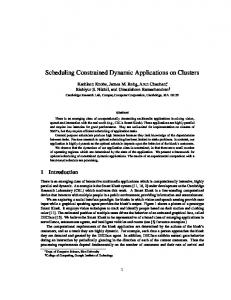
2.2 SI techniques for Cloud scheduling Due to the fact that artificial life techniques have been effective in combinational optimization problems, they result good alternatives to achieve the goals proposed in this work. SI represents a set of artificial life techniques that has received increasing attention for solving this type of problems [7]. The advantage of SI derives from their ability to explore solutions in large search spaces in a very efficient way. All in all, using SI techniques remains an interesting approach to cope in practice with the NP-completeness of job scheduling problems. Particularly, the ACO algorithm [6] arise from the way real ants behave in nature, i.e., from the observation of ant colonies when they search the shortest paths to reach a food source from their nest. In nature, real ants move randomly from one place to another to search for food, and upon finding food and returning to their nest each ant leaves a pheromone that lures other working ants to the same course. When more and more ants choose the same path, the pheromone trail is reinforced and even more ants will further choose it. This positive feedback eventually leaves all the ants following a single path. Over time the shortest paths will be intensified by the pheromone faster since the ants will both reach the food source and travel back to their nest faster. However, if over time ants do not visit a certain path, pheromone trails start to evaporate, thus reducing their attractive strength. The more the time an ant needs to travel down the path and back again, the less the pheromone trails are reinforced. From an algorithmic point of view, the pheromone evaporation process is useful for avoiding the convergence to a local optimum solution. Figure 2 shows two possible nest-food source paths, but one of them is longer than the other one. Figure 2 (a) shows how ants will start moving randomly at the beginning to explore the ground and then choose one of two paths. The ants that follow the shorter path will naturally reach the food source before the others ants, and in doing so the former group of ants will leave behind them a pheromone trail. After reaching the food, the ants will turn back and try to find the nest. Moreover, the ants that perform the round trip faster, strengthen more quickly the quantity of pheromone in the shorter path, as shown in Figure 2 (b). The ants that reach the food source through the slower path will find attractive to return to the nest using the shortest path. Eventually, most ants will choose the left path as shown in Figure 2 (c). In the ACO algorithm, at each execution step, ants compute a set of feasible moves and select the best one (according to some probabilistic rules) to carry out all the tour. The transition probability for moving from a place to another is based on the heuristic information and pheromone trail level of the move. The higher the value of the pheromone and the heuristic information, the more profitable it is to select this move and resume the search. All ACO algorithms adapt the algorithm scheme explained next. After initializing the pheromone trails and control parameters, a main loop is repeated until a stopping criterion is met (e.g., a certain number of iterations to perform or a given time limit without improving the result). In the main loop of the algorithm ants construct feasible 6

Figure 2: Adaptive behaviour of ants solutions and update the associated pheromone trails. Furthermore, partial problem solutions are seen as nodes (an abstraction for the location of an ant): each ant starts to travel from a random node and moves from a node i to another node j of the partial solution. At each step, the ant k computes a set of feasible solutions to its current node and moves according to a probability distribution. For an ant k the probability τij .ηij pkij to move from a node i to a node j is pkij = P q∈allowed if j ∈ allowedk , or k τiq ηiq pkij = 0 otherwise. ηij is the attractiveness of the move as computed by some heuristic information indicating a prior desirability of that move. τij is the pheromone trail level of the move, indicating how profitable it has been in the past to make that particular move (it represents therefore a posterior indication of the desirability of that move). Finally, allowedk is the set of remaining feasible nodes. To conclude, the higher the pheromone value and the heuristic information, the more profitable it is to include state j in the partial solution. The initial pheromone level is a positive integer τ0 . In nature, there is not any pheromone on the ground at the beginning (i.e., τ0 = 0). However, the ACO algorithm requires τ0 > 0, otherwise the probability to chose the next state would be pkij = 0 and the search process would stop from the beginning. Furthermore, the pheromone level of the elements of the solutions is changed by applying an update rule τij ← ρ.τij + ∆τij , where 0 < ρ < 1 models pheromone evaporation and ∆τij represents additional added pheromone. Normally, the quantity of the added pheromone depends on the quality of the solution.

3 Proposed scheduler Conceptually, the scheduling problem can be formulated as follows. A number of users are connected to the Cloud at different times to execute their PSEs. To perform this, each user requests to the Cloud the creation of v VMs. A PSE is formally defined as a set of N = 1, 2, ..., n independent jobs, where each job corresponds to a particular value for a variable of the model being studied by the PSE. The jobs are distributed and executed on the v machines created by the corresponding user. Due to the fact that the total number of VMs required by all users is greater than the number 7

of Cloud physical resources (i.e., hosts), a strategy that achieves a good use of these physical resources must be implemented. This strategy is implemented at the Datacenter (or Cloud infrastructure) level by means of a support that allocates user VMs to hosts. Moreover, a strategy for assigning user jobs to allocated VMs is also necessary (currently we use FIFO). In short, our scheduler operates at two levels: Cloud infrastructure and VM. To implement the Cloud-level part of the scheduler, AntZ, the algorithm proposed in [16] to solve the problem of load balancing in Grid environments has been adapted to be used in Clouds (see algorithm in Table 1 (left)). AntZ combines the idea of how ants cluster objects with their ability to leave pheromone trails on their paths so that it can be a guide for other ants passing their way. In our adapted algorithm, each ant works independently and represents a VM “looking” for the best host to which it can be allocated. The main procedure performed by an ant is shown in Table 1 (left). When a VM is created, an ant is initialized and starts to work. A master table containing information on the load of each host is initialized (initializeLoadTable()). Subsequently, if an ant associated to the VM that is executing the algorithm already exists, the ant is obtained from a pool of ants through the getAntPool(vm) method. If the VM does not exist in the ant pool, then a new ant is created. To do this, first, a list of all suitable hosts in which can be allocated the VM is obtained. A host is suitable if it has an amount of processing power, memory and bandwidth greater than or equal to that of required by the unallocated VM. Then, the working ant and its associated VM is added to the ant pool (antPool.add(vm,ant)) and the ACO-specific mechanism starts to operate (see algorithm in Table 2 (left)). In each iteration of the sub-algorithm, the ant collects the load information of the host that is visiting –through the getHostLoadInformation() operation– and adds this information to its private load history. The ant then updates a load information table of visited hosts (localLoadTable.update()), which is maintained in each host. This table contains information of the own load of an ant, as well as load information of other hosts, which were added to the table when other ants visited the host. Here, load refers to the total CPU utilization within a host and is calculated taking into account the number of VMs that are executing at any moment in each physical host. To calculate the load, the original AntZ algorithm receives the number of jobs that are executing in the resource in which the load is being calculated, and it is calculated taking into account the amount available of million instructions per second (MIPS) in each CPU. MIPS is a metric that indicates how fast a computer processor runs. In our proposed algorithm, the load is calculated on each host taking into account the CPU utilization made by all the VMs that are executing on each host. This metric is useful for an ant to choose the least loaded host to allocate its VM. When an ant moves from one host to another it has two choices: moving to a random host using a constant probability or mutation rate, or using the load table information of the current host (chooseNextStep()). The mutation rate decreases with a decay rate factor as time passes, thus, the ant will be more dependent on load in-

8

Procedure A C O a l l o c a t i o n P o l i c y ( vm , h o s t L i s t ) Begin initializeLoadTable () a n t = g e t A n t P o o l ( vm ) i f ( a n t == n u l l ) t h e n suitableHosts= g e t S u i t a b l e H o s t s F o r V m ( h o s t L i s t , vm ) a n t =new Ant ( vm , s u i t a b l e H o s t s ) a n t P o o l . add ( vm , a n t ) end i f repeat ant . AntAlgorithm ( ) until ant . isFinish () allocatedHost = h o s t L i s t . get ( ant . getHost ( ) ) i f ( ! a l l o c a t e d H o s t . a l l o c a t e V M ( a n t . getVM ( ) ) ) repeat A C O a l l o c a t i o n P o l i c y ( a n t . getVM ( ) , h o s t L i s t ) n u m b e r O f R e t r i e s −− u n t i l s u c e s s f u l l or n u m b e r O f R e t r i e s ==0 End

Procedure SubmitJobsToVMs ( j o b L i s t ) Begin vmIndex =0 while ( j o b L i s t . s i z e ( ) > 0) job= j o b L i s t . getNextJob ( ) vm= g e t V M s L i s t ( vmIndex ) vm . scheduleJobToVM ( j o b ) totalVMs=getVMsList ( ) . s i z e ( ) vmIndex =Mod( vmIndex +1 , t o t a l V M s ) j o b L i s t . remove ( j o b ) end w h i l e End

Table 1: ACO-based allocation algorithm for individual VMs (left) and the SubmitJobsToVMs procedure (right)

formation than to random choice. This process is repeated until the finishing criterion is met. The completion criterion is equal to a predefined number of steps (maxSteps). Finally, the ant delivers its VM to the current host and finishes its task. Due to the fact that each step performed by an ant involves moving through the network, we have added a control to minimize the number of steps that an ant performs: every time an ant visits a host that has not yet allocated VMs, then the ant allocates its associated VM to it directly without performing further steps. When the ant has not completed its work, i.e., the ant can not allocate its associated VM to a host, then an exponential back-off strategy is activated. The allocation of each failing VM in the queue is re-attempted every s seconds and retried n times. Every time an ant visits a host, it updates the host load information table with the information of other hosts, but at the same time the ant collects the information already provided by the table of that host, if any. The load information table acts as a pheromone trail that an ant leaves while it is moving, to guide other ants to choose better paths rather than wandering randomly in the Cloud. Entries of each local table are the hosts that ants have visited on their way to deliver their VMs together with their load information. When an ant reads the information in the load table in each host through and chooses a direction via the algorithm in Table 2 (right), the ant chooses the lightest loaded host in the table, i.e., each entry of the load information table is evaluated and compared with the current load of the visited host. If the load of the visited host is smaller than any other host provided in the load information table, the ant chooses the host with the smallest load. On the other hand, if the load of the visited host is equal to any host in the load information table, the ant chooses a host randomly. Once the VMs have been allocated in physical resources, the scheduler proceeds to assign the jobs to these VMs. To do this, jobs are assigned to VMs according 9

Procedure A n t A l g o r i t h m ( ) Begin s t e p =1 initialize () While ( s t e p < m a x S t e p s ) do currentLoad=getHostLoadInformation () A n t H i s t o r y . add ( c u r r e n t L o a d ) localLoadTable . update ( ) i f ( currentLoad = 0.0) break else i f ( random ( ) < m u t a t i o n R a t e ) t h e n nextHost =randomlyChooseNextStep ( ) else nextHost=chooseNextStep ( ) end i f m u t a t i o n R a t e = m u t a t i o n R a t e −d e c a y R a t e s t e p = s t e p +1 moveTo ( n e x t H o s t ) end w h i l e deliverVMtoHost ( ) End

Procedure C h o o s e N e x t S t e p ( ) Begin bestHost=currentHost bestLoad=currentLoad for each e n t r y in h o s t L i s t i f ( e n t r y . l o a d < bestLoad ) then bestHost=entry . host e l s e i f ( e n t r y . l o a d = bestLoad ) then i f ( random . n e x t < p r o b a b i l i t y ) t h e n bestHost=entry . host end i f end i f end f o r End

Table 2: ACO-specific logic: Core logic (left) and ChooseNextStep procedure (right) to the algorithm in Table 1 (right). This represents the second scheduling level of the scheduler proposed as a whole. This sub-algorithm uses two lists, one containing the jobs that have been sent by the user, i.e., a PSE, and the other list contains all user VMs that are already allocated to a physical resource and hence are ready to execute jobs. The algorithm iterates the list of all jobs –jobList– and then, through getNextJob() method retrieves jobs by a FIFO policy. Each time a job is obtained from the jobList it is submitted to be executed in a VM in a round robin fashion. The VM where the job is executed is obtained through the method getVMsList(vmIndex). Internally, the algorithm maintains a queue for each VM that contains its list of jobs to be executed. The procedure is repeated until all jobs have been submitted for execution, i.e., when the jobList is empty.

4 Evaluation To assess the effectiveness of our proposal in a non-batch Cloud environment where multiple users are dynamically connected to execute their PSEs, we have processed a real case study for solving a well-known benchmark problem discussed for instance in [2]. The experimental methodology involved two steps. First, we executed the problem in a single machine by varying an individual problem parameter by using a finite element solver, which allowed us to gather real job processing times and input/output data sizes (see Section 4.1). Then, by means of the generated job data, we instantiated the CloudSim simulation toolkit, which is explained in Section 4.2. The obtained results regarding the performance of our proposal compared to some Cloud scheduling alternatives are reported in Section 4.3. 10

4.1 Real job data gathering The problem considered in Garc´ıa Garino et al. [2] involves studying a plane strain plate with a central circular hole. The dimensions of the plate were 18 x 10 m, with R = 5 m. Material constants were E = 2.1 105 Mpa, ν = 0.3, σy = 240 Mpa and H = 0. A linear Perzyna viscoplastic model with m = 1 and n = ∞ was considered. Unlike previous studies of our own [17], in which a geometry parameter was chosen to generate the PSE jobs, in this case a material parameter was selected as the variation parameter. Then, 20 different viscosity values for the η parameter were considered, namely α ∗ 10β (with α = 1, 2, 3, 4, 5, 7 and β = 4, 5, 6) in addition 1.107 and 2.107 Mpa. Details on viscoplastic theory and numerical implementation considered can be found in [2]. The finite element mesh used has 1,152 elements and Q1/P0 elements were chosen. Imposed displacements (at y=18m) were applied until a final displacement of 2,000 mm was reached in 400 equal time steps of 0.05 mm each. It is worth noting that ∆t = 1 has been set for all the time steps. After establishing the problem parameters, we employed a single machine to run the parameter sweep experiment by varying the viscosity parameter η as indicated and measuring the execution time for the 20 different experiments, which resulted in 20 input files with different input configurations and 20 output files. The tests were solved using the SOGDE finite element software [2, 18]. Furthermore, the machine on which the tests were carried out had an AMD Athlon(tm) 64 X2 Dual Core Processor 3600+, with 2 GBytes of RAM, 400 Gbytes of storage, and a bandwidth of 100 Mbps. The machine was equipped with the Linux operating system (specifically an Ubuntu 11.04 distribution) running the generic kernel version 2.6.38-8. The information regarding machine processing power was obtained from the native benchmarking support of Linux and as such is expressed in MIPS. The machine had 4,008.64 MIPS. It is worth noting that only one core was used during the experiments. Once the execution times were obtained from the real machine, we approximated for each experiment the number of executed instructions by the following formula N Ii = mipsCP U ∗Ti , where N Ii is the number of million instructions to be executed by or associated to a job i, mipsCP U is the processing power of the CPU of our real machine measured in MIPS, and Ti is the time that took to run the job i on the real machine. For example, for a 117-second job, the approximated number of instructions for the job was 469,011 million instructions.

4.2 CloudSim instantiation First, the CloudSim simulator [10] was configured with a datacenter composed of a single machine –or “host” in CloudSim terminology– with the same characteristics as the real machine where the experiments were performed. As such, the characteristics were 4,008 MIPS (processing power), 4 GBytes (RAM), 400 GBytes (storage), 100 Mbps (bandwidth), and 4 CPUs. Each CPU had the same processing power. Once configured, and to ensure significance, we checked that the simulated ex11

ecution times were close to real times for each independent job performed on the real machine, which was successful. Once the single-machine execution times from CloudSim were validated, a new simulation scenario was set. This new scenario consisted of a datacenter with 10 hosts, where each has the same hardware capabilities as the real single machine. Then, each user connecting to the Cloud requests v VMs to execute their PSE. Each VM has one virtual CPU of 4,008 MIPS, 512 Mbyte of RAM, a machine image size of 100 Gbytes and a bandwidth of 5 Mbps. This is a moderatelysized, homogeneous datacenter that can be found in many real scenarios [19]. To evaluate the performance in the simulated Cloud we have modeled a dynamic Cloud scenario in which new users connect to the Cloud every 120 seconds, and requires the creation of 10 VMs in which run their PSE –a set of 80 jobs–. This is, the real base job set comprising 20 jobs that was obtained by varying the value of η was cloned to obtain more jobs. The number of users who connect to the Cloud varies as u = 10, 20, ..., 120, and since each user executes one PSE –80 jobs–, the total number of jobs to execute is increased as n = 80 ∗ u each time. Each job, called cloudlet by CloudSim, was determined by a length parameter or the number of instructions to be executed by the cloudlet, which varied between 244,527 and 469,011. Moreover, another parameter was PEs, or the number of processing elements (cores) required to perform each individual job. Each cloudlet required one PE since jobs are sequential (not multi-threaded). Finally, the experiments had input files of 93,082 bytes and output files of 2,202,010 bytes. In CloudSim, the amount of available hardware resources for each VM is constrained by the total processing power, RAM, storage and system bandwidth available within the associated host. Thus, scheduling policies must be applied to properly assign VMs to hosts and achieve efficient use of resources. In addition, CloudSim allows users to easily configure different VM scheduling policies. This allowed us to experiment with the scheduler proposed in this paper and compare it against CloudSim built-in schedulers. The next section explains the associated obtained results in detail.

4.3 Performed experiments In this subsection we report on the obtained results when executing PSEs submitted by multiple users in the simulated Cloud by using our two-level scheduler and alternative Cloud scheduling policies for assigning VMs to hosts and handling jobs. Due to their high CPU requirements, and the fact that each VM requires only one PE, we assumed a 1-1 job-VM execution model, i.e., jobs within a VM waiting queue are executed one at a time by competing for CPU time with other jobs from other VMs in the same hosts. This is, a time-shared CPU scheduling policy was used, since it is a good alternative for executing CPU-intensive jobs in terms of fairness. Moreover, our proposed algorithm is compared against another three schedulers: • Random, a simple scheduling algorithm in which the VMs requested by the different users are assigned randomly to different physical resources. Although this algorithm does not provide an elaborated criterion to allocate the VMs to 12

physical resources, it provides a good benchmark in order to compare and see how our proposed VM allocation algorithm performs compared to random assignment. • A scheduler based on genetic algorithm (GA) proposed in [9], also evaluated via CloudSim, in which the population structure is represented as the set of physical resources that compose a datacenter, as illustrated in Figure 3. Each chromosome is an individual in the population that represents a part of the searching space. Each gene (field in a chromosome) is a host in the Cloud, and the last field in this structure is the fitness field. For each request to allocate a VM, this fitness field is updated in each chromosome. The fitness field indicates the result of the fitness function and it is calculated as the inverse of the accumulated load of all hosts composing the chromosome. The load in each is host is calculated taking into account the number of VMs that are executing in it. A chromosome with higher fitness indicates that its associated set of hosts has the most free CPUs to perform the current allocation. Queue of requests to allocations VM2

VM1

...

VMn

Fitness to current VM allocation

Host combinations chromosome

1

6

...

4

3

6

Population

5

3

7

H1

H2

H3

...

2

8

Hm

Fitness

Figure 3: Genetic encoding of VM scheduling to physical hosts Each chromosome keeps combinations of hosts and the fitness of the current allocation. In each generation, a new population P2 originated from the initial population P is formed by selecting chromosomes using a Roulette method [20], given a probability of selection proportional to the chromosome fitness. This P2 population is recombined using a crossover uniform with the aim of exploring more possible servers with better fitness to the current allocation. The evaluation step is done over the P2 population to update the fitness field of this new recombined population. Chromosomes with low fitness in P are replaced by the better individuals in P2. Thus, the algorithm preserves the best individuals to increase the probability of a better allocation. At the end of generations, two sorting steps are done: one local to provide a sorted list of hosts in the chromosome with higher fitness, and a global sort, to provide a sorted list of individuals 13

with better fitness. The allocation of VMs will begin in the first host of the first chromosome. If this host is not able to perform this operation, the next host in the chromosome with better fitness is selected. In the experiments, the GAspecific parameters were set with the following values: chromosome size = 8, population size = 10 and number of iterations = 10. • Min-Min, a policy that chooses, as the host for a VM, the host with less PEs in use. Every time a user requests the allocation of a VM, the broker sends a message to all hosts to know their states and get one with less PEs in use. A broker represents an entity acting on behalf of a user. A broker hides the VM management, such as VM creation, submission of jobs to the created VMs and destruction of VMs. On the other hand, the state of a resource represents the number of free PEs. This algorithm was implemented as an ideal scheduler that always achieves the best possible allocation of VMs to physical resources. To achieve allocate all the VMs, the scheduler performs by using a back-off strategy many attempts to create VMs as needed until it reaches to serve all users. The number of needed retries to serve all users was set equal to 20. This scheduler has been implemented in this way to obtain the ideal values to which all its competitors, including ACO, should be compared against. In our ACO scheduler, we have set the ACO-specific parameters with the following values: mutation rate = 0.6, decay rate = 0.1 and maximum steps = 8. In all cases, the considered algorithms use the same VM-level policy for handling jobs within VMs (i.e., FIFO with round robin), and the VMs allocated to a single host (i.e., timeshared [4]). Moreover, using time-shared means there is not limit on the number of VMs a host can handle. To achieve allocate the VMs to hosts, each scheduler must make a different number of queries to hosts to determine their availability each time they attempting to allocate a VM. These queries are performed through messages sent over the network to hosts to obtain information regarding their availability. For example, Min-Min needs to send messages to hosts every time a VM is allocated to know the hosts states and to decide where to allocate the VM. Moreover, as mentioned earlier, Min-Min performs a number of creation retries until all users are served, which makes the number of messages to send even higher. This process is not actually modeled in CloudSim, but the number of messages sent every time the allocation of a VM is performed should be equal to the total number of physical resources, i.e., sending a message for each host to get the number of free PEs so as to allocate the VM to the host that has the highest number of free PEs. Because the current implementation of Min-Min keeps a vector containing free PEs information for each host, and the algorithm assumes that these PEs are exclusive to PSE job processing and can not be allocated externally (i.e., by computations external to the Cloud owner), Min-Min always can do the best possible allocation since it has information beforehand. In this work we consider Min-Min as the best opponent to which we can compare our scheduler against. It is important to note, however, that the 14

Min-Min implementation was executed using the back-off strategy with a number of retries equal to 20 to obtain the ideal values to reach. Furthermore, since the GA algorithm contains a population size of 10 and chromosome sizes of 8 (7 genes for hosts plus one gene for the fitness value), to calculate the fitness function, the algorithm should send one message for each host of the chromosome to know the availability and obtain the chromosome containing the best fitness value. The VM is allocated in a host belonging to the chromosome with the best fitness value. The number of messages to send will be equal to the number of host within each chromosome multiplied by the population size. Finally, the last competitor in this work is Random, which sends only one network message to a random host for each attempt of VM creation. It is worth to consider, however, that our ACO algorithm makes less use of the network resources than GA and Min-Min. For this, we have set the maximum number of steps that an ant carries out to allocate a single VM to 8, i.e., ACO sends a maximum of 8 messages per VM allocation versus the 10 messages Min-Min and 7x10 messages GA would send if properly simulated or implemented. When ACO finds an unloaded host allocates a VM and does not perform any further step. For the configuration of our proposed scenario this reduction in the number of steps, i.e., messages, is an improvement in network usage of 20% in terms of transmitted messages with respect to Min-Min without to use the back-off strategy. Although Random would send less messages, it is an inefficient algorithm because creates less VMs and offers the lowest job rate among all the users it serves. In our previous works [8, 5], a batch mode scenario was considered and the goal was minimizing the flowtime and makespan of all jobs submitted by one user. In this work, unlike [8, 5], an online Cloud scenario is evaluated. An online Cloud is a Cloud which is available all the time and to which different users connect at different times to submit their experiments. Furthermore, in an online Cloud, the rate at which jobs are processed is as important as processing all users requests. It is for this reason that the goals to achieve have been redefined compared to [5]. To evaluate job rate execution, and since each competing algorithm is capable of actually executing different numbers of jobs, we have used alternative metrics other than makespan and flowtime to compare scheduler performance. Below, the experiments have been performed with the aim of maximizing the tradeoff between the number of serviced users by the Cloud –among all users that are connected to the Cloud– and the jobs that have been executed per unit time up to the time a new user connects to the Cloud. The number of executed jobs –job rate– at time t was calculated as N umberJobst=0,120,240,... = T otalN umberExecutedJobst − T otalN umberExecutedJobst−1 . Irrespective of the metric, in this work we show average results , which arise from averaging 10 times the execution of each algorithm. Figures 4, 5 and 6 illustrate the number of serviced users by the Cloud, the number of executed jobs per unit time and the number of created VMs by each algorithm, respectively. In all cases, each user is connected to the Cloud every 120 seconds. Subfigures in Figures 4, 5 and 6 represent the scenarios in which an exponential back-off strategy to wait for a while is performed to try reallocate VMs whose allocation failed.

15

Without retries of VMs creation 120

With 3 retries of VMs creation

ACO GA Random Min−Min

120

100 Number of serviced users

Number of serviced users

100

ACO GA Random Min−Min

80

60

40

20

80

60

40

20

0

0 10

20

30

40

50

60

70

80

90

100

110

120

10

20

30

40

Number of users online

50

60

70

80

90

100

110

120

Number of users online

Figure 4: Results as the number of users online increases: Number of serviced users Without retries of VMs creation

Number of executed jobs (More is better)

50

With 3 retries of VMs creation 60

ACO GA Random Min−Min

50 Number of executed jobs (More is better)

60

40

30

20

10

ACO GA Random Min−Min

40

30

20

10

0

0 10

20

30

40

50

60

70

80

90

100

110

120

10

Number of users online

20

30

40

50

60

70

80

90

100

110

120

Number of users online

Figure 5: Results as the number of users online increases: Number of executed jobs per unit time This strategy is activated every 120 seconds and the number of retries are 0 (no retry) and 3 times, respectively. The reason that the schedulers can not serve all users that connect to the Cloud is because the attempt to create VMs fails when the user requests them. This is, at the moment a user issues the creation, all physical resources are already fully busy with VMs belonging to other users. Depending on the algorithm and according to the results, some schedulers are able to find to some extent a host with free resources to which at least one VM per user is allocated. It is for this reason that in this work we have also incorporated the mechanism to retry to improve both the number of serviced users by the Cloud as the number of VMs that are created for each of them. Among all approaches, excluding Min-Min which is only taken as reference of an ideal performance to reach, GA is the algorithm that serves less users but creates more VMs and executes a number of jobs per unit time (job rate) greater than Random and ACO. This is because the population size is equal to 10, and each chromosome contains 7 different hosts, so after 10 iterations GA always finds the hosts with better fitness, and can thus allocate more VMs to the first users who connect to the Cloud. On the other hand, Random serves more users than ACO –in some cases– and GA –in 16

Without retries of VMs creation 1200

With 3 retries of VMs creation

ACO GA Random Min−Min

1200

1000 Number of created VMs

Number of created VMs

1000

ACO GA Random Min−Min

800

600

400

200

800

600

400

200

0

0 10

20

30

40

50

60

70

80

90

100

110

120

10

Number of users online

20

30

40

50

60

70

80

90

100

110

120

Number of users online

Figure 6: Results as the number of users online increases: Number of created VMs

all cases– but with the lowest job rate and less VMs. It is important to note that, while Random serves many users, it may not be fair with the response times for users. The reason behind this is that the Random algorithm assigns the VMs to physical resources randomly, and many of the creations of the VMs requested by users might fail. There are situations where for a single user Random is able to create only one VM where all jobs of the user are executed. This situation means that the user must wait too long to complete their jobs and thus loses the benefit of using a Cloud. Finally, ACO performs the best balance with respect to all metrics in question. The ACO scheduler is the algorithm that better balances both the number of serviced users, the number of executed jobs per unit time and the total number of created VMs. ACO achieves the best trade-off between the number of serviced users and the number of executed jobs and created VMs with respect to GA. Moreover, unlike GA, ACO improves the number of serviced users when the number of retries to create VMs increases. On the other hand, ACO offers the best trade-off between the number of executed jobs per unit time and the number of created VMs with respect to the number of serviced users of Random. To visualize how ACO achieves a better balance of the proposed metrics in this paper, the results obtained from different algorithms have been normalized to calculate a new weighted metric. The normalized values for each metric and each user group U connected to the Cloud were calculated as N ormalizedV alueUi=10,20,...,120 = 1 − (M ax(valueUi ) − valueUi )/(M ax(valueUi ) − M in(valueUi ). Table 3 summarizes a weighted metric calculated from the normalized values obtained from each algorithm –ACO, GA, Random and Min-Min– and are calculated by: M etricW eightedUi=10,20,..,120 = (weightSU ∗ N ormalSU i + weightEJ ∗ N ormalEJ + weightV M s ∗ N ormalV M sUi + weightJR ∗ N ormalJRUi ), where weightSU is the weight applied to the number of serviced users, weightEJ weighs the total number of executed jobs (this value is equal to the sum of jobs sent by each serviced user, i.e., the total number of jobs that were executed), weightVMs weighs the number of created VMs and weightJR weighs the number of executed job per unit time. Since all metrics are important and they are to be balanced, we have assigned all 17

Without retries

Users connected to the Cloud

With 3 retries

ACO

GA

Random

Min-Min

ACO

GA

Random

Min-Min

10

0.39

0.26

0.10

1

0.48

0.22

0.34

1

20

0.38

0.29

0.33

1

0.32

0.31

0.15

1

30

0.35

0.30

0.30

1

0.33

0.30

0.17

1

40

0.24

0.25

0.23

1

0.25

0.23

0.14

1

50

0.30

0.24

0.24

1

0.19

0.17

0.13

1

60

0.32

0.27

0.23

1

0.27

0.22

0.15

1

70

0.30

0.28

0.19

1

0.30

0.21

0.14

1

80

0.26

0.25

0.18

1

0.26

0.17

0.14

1

90

0.31

0.21

0.18

1

0.19

0.16

0.13

1

100

0.37

0.25

0.07

1

0.18

0.14

0.13

1

110

0.24

0.23

0.07

1

0.23

0.14

0.14

1

120

0.25

0.21

0.08

1

0.25

0.14

0.13

1

Table 3: Weighted metric weights equally, i.e., equal to 0.25. The higher the value of the weighted metric, the better the metric balance of an algorithm with respect its competitors. Excluding Min-Min, which is shown as a reference of the ideal values to reach, some observations are that when the VMs are created without retries as in Table 3, in most cases the weighted metric is more favorable to ACO, giving better values with regard to their competitors –Random and GA– eleven times out of twelve times. On the other hand, when the number of retries is equal to 3, ACO again achieves the best balance with respect to its competitors in all cases. As shown in these experiments, ACO is the algorithm that achieves a better tradeoff between the number of serviced users and the executed jobs rate per unit time creating a reasonable number of VMs for each of them. This is, the weighted metric shows that ACO is the algorithm that achieves the best balance among all the proposed metrics, specially when three retries are used. Min-Min has only been treated in these experiments as fictitious algorithm that gets ideal results but is taken only as a reference to determine how far each competitor is from the former. To conclude it is important to note that both Min-Min and GA make a greater use of network than ACO. On the other hand, Random sends few messages but it does not show a good performance. These results are encouraging because they indicate that ACO is very close to obtaining the best possible solution balancing all the employed evaluation metrics and making a reasonable use of the network resources. These observations might impact on performance if properly modelled in the simulation. 18

5 Conclusions PSEs is a type of simulation that involves running a large number of independent jobs and typically requires a lot of computing power. These jobs must be efficiently processed in the different computing resources of a parallel environment such as the ones offered by a Cloud. Then, job scheduling plays a fundamental role. Recently, SI-inspired algorithms have received increasing attention in the research community. SI refers to the collective behaviour that emerges from a swarm of social insects. Social insect colonies collectively solve complex problems by intelligent methods. These problems are beyond the capabilities of each individual insect, and the cooperation among them is self-organized without any supervision. Through studying social insect behaviours such as ant colonies, researchers have proposed algorithms for combinatorial optimization problems, and consequently Cloud schedulers. Existing efforts do not address in general dynamic, online environments where multiple users connect to scientific Clouds to execute their PSEs and to the best of our knowledge, no effort aimed at balancing the number of serviced users in a Cloud and the number of executed jobs for each joining user. Executing a greater number of jobs every time a user connects means a more agile human processing of PSE job results. Therefore, our proposed two-level Cloud scheduler pays special attention to this aspect and the total number of serviced users and the number of created VMs. Simulated experiments performed with the help of the well-established CloudSim toolkit and real PSE job data show that our scheduler provides a better balance to the trade-off between the number of serviced users and the job execution rate by user. Moreover, ACO improves in the number of serviced users when the back-off strategy is applied to retry creating the VMs that failed in their first attempt to creation. We are extending this research line in several directions. First, we plan to materialize the resulting schedulers on top of a real Cloud platform, such as Emotive Cloud (http://www.emotivecloud.net/) or OpenNebula (http://opennebula. org/), which are designed for extensibility. Second, we will consider other Cloud scenarios, for example, with heterogeneous machines. Lastly, we will evaluate and measure how the variation of the parameters of each algorithm (e.g., maxSteps, mutation rate and decay rate in ACO, chromosome size, population size and number of iterations in GA) influence the performance and network consumption. For instance, the more the maxSteps in our ACO scheduler, the more the “migrations” of ants among Cloud hosts, which increases network consumption. Another issue concerns energy consumption by the scheduler itself. Simple schedulers (e.g., Random or Min-Min) require less CPU usage and memory accesses compared to more complex policies such as our scheduler. For example, we need to maintain host load information for ants, which requires those resources. Therefore, when running many jobs, the accumulated resource usage overhead may be considerable for large Cloud infrastructures, resulting in higher demands for energy. Another research line is the allocation of VMs of different users to physical resources belonging to federated Clouds taking into account not only processing re19

quirements in the domain but also the interconnection capacity –network links– of the domains. A federated Cloud includes multiple Cloud providers devoted to create an uniform Cloud resource interface to users. Indeed, in [9] a GA-based solution for the problem has been proposed, and we aim at applying ACO as well.

References [1] C. Youn, T. Kaiser, “Management of a parameter sweep for scientific applications on cluster environments”, Concurrency & Computation: Practice & Experience, 22: 2381–2400, 2010. [2] C. Garc´ıa Garino, M. Ribero Vairo, S. And´ıa Fag´es, A. Mirasso, J.P. Ponthot, “Numerical simulation of finite strain viscoplastic problems”, Journal of Computational and Applied Mathematics, 2012, In press. [3] R. Buyya, C. Yeo, S. Venugopal, J. Broberg, I. Brandic, “Cloud computing and emerging IT platforms: Vision, hype, and reality for delivering computing as the 5th utility”, Future Generation Computer Systems, 25(6): 599–616, 2009. [4] E. Pacini, M. Ribero, C. Mateos, A. Mirasso, C. Garc´ıa Garino, “Simulation on Cloud Computing Infrastructures of Parametric Studies of Nonlinear Solids Problems”, in F.V. Cipolla-Ficarra et al. (Editor), Advances in New Technologies, Interactive Interfaces and Communicability (ADNTIIC 2011), Volume 7547 of LNCS, pages 58–70. Springer-Verlag, 2011, ISBN 978-3-642-34009-3. [5] C. Mateos, E. Pacini, C. Garc´ıa Garino, “An ACO-inspired Algorithm for Minimizing Weighted Flowtime in Cloud-based Parameter Sweep Experiments”, Advances in Engineering Software, 56: 38–50, 2013. [6] E. Bonabeau, M. Dorigo, G. Theraulaz, Swarm Intelligence: From Natural to Artificial Systems, Oxford University Press, 1999. [7] E. Pacini, C. Mateos, C. Garc´ıa Garino, “Schedulers based on Ant Colony Optimization for Parameter Sweep Experiments in Distributed Environments”, in Dr. Siddhartha Bhattacharyya, Dr. Paramartha Dutta (Editor), Handbook of Research on Computational Intelligence for Engineering, Science and Business, Volume I, Chapter 16, pages 410–447. IGI Global, 2012, ISBN13: 9781466625181. [8] C. Garc´ıa Garino, C. Mateos, E. Pacini, “Job scheduling of parametric computational mechanics studies on cloud computing infrastructures”, International Advanced Research Workshop on High Performance Computing, Grid and Clouds. Cetraro (Italy). Available online: http://www.hpcc.unical.it/hpc2012/pdfs/garciagarino.pdf, June 2012. [9] L. Agostinho, G. Feliciano, L. Olivi, E. Cardozo, E. Guimaraes, “A Bio-inspired Approach to Provisioning of Virtual Resources in Federated Clouds”, in Ninth International Conference on Dependable, Autonomic and Secure Computing (DASC), DASC 11, pages 598–604. IEEE Computer Socienty, Washington, DC, USA, 12-14 December 2011, ISBN: 978-0-7695-4612-4. [10] R. Calheiros, R. Ranjan, A. Beloglazov, C. De Rose, R. Buyya, “CloudSim: A Toolkit for Modeling and Simulation of Cloud Computing Environments and 20

[11]

[12]

[13]

[14]

[15]

[16] [17]

[18]

[19]

[20]

Evaluation of Resource Provisioning Algorithms”, Software: Practice & Experience, 41(1): 23–50, 2011. M. Armbrust, A. Fox, R. Griffithn, A. Joseph, R. Katz, A. Konwinski, G. Lee, D. Patterson, A. Rabkin, I. Stoica, M. Zaharia, “Above the Clouds: A Berkeley view of Cloud Computing”, Technical Report UCB/EECS-2009-28, EECS Department, University of California, Feb 2009. B. Sotomayor, K. Keahey, I. Foster, T. Freeman, “Enabling Cost-Effective Resource Leases with Virtual Machines”, in Hot Topics session in ACM/IEEE International Symposium on High Performance Distributed Computing 2007. Monterey Bay, CA (USA), 2007. L. Cherkasova, D. Gupta, A. Vahdat, “When virtual is harder than real: Resource allocation challenges in virtual machine based IT environments”, Technical report, HP Laboratories. Technical Report HPL-2007-25, Palo Alto, February 2007. L. Wang, J. Tao, M. Kunze, A.C. Castellanos, D. Kramer, W. Karl, “Scientific Cloud Computing: Early Definition and Experience”, in 10th IEEE International Conference on High Performance Computing and Communications, pages 825– 830. IEEE Computer Society, Washington, DC, USA, 2008. W. Huang, J. Liu, B. Abali, D. Panda, “A case for high performance computing with virtual machines”, in Proceedings of the 20th annual international confer´ pages 125–134. ACM, New York, NY, USA, ence on Supercomputing, ICS 06, 2006, ISBN: 1-59593-282-8. S. Ludwig, A. Moallem, “Swarm Intelligence Approaches for Grid Load Balancing”, Journal of Grid Computing, 9(3): 279–301, 2011. C. Careglio, D. Monge, E. Pacini, C. Mateos, A. Mirasso, C. Garc´ıa Garino, “Sensibilidad de Resultados del Ensayo de Tracci´on Simple Frente a Diferentes Tama˜nos y Tipos de Imperfecciones”, in M.G. E. Dvorkin, M. Storti (Editors), Mec´anica Computacional, Volume XXIX, pages 4181–4197. AMCA, 2010. C. Garc´ıa Garino, F. Gabald´on, J.M. Goicolea, “Finite Element Simulation of the Simple Tension Test in Metals”, Finite Elements in Analysis and Design, 42 (13): 1187–1197, 2006. C. Mateos, A. Zunino, M. Campo, “On the evaluation of gridification effort and runtime aspects of JGRIM applications”, Future Generation Computer Systems, 26(6): 797 – 819, 2010. A. Lipowski, D. Lipowska, “Roulette-wheel selection via stochastic acceptance”, Physica A: Statistical Mechanics and its Applications, 391(6): 2193– 2196, 2012.

21