the actual execution time is always less or equal to the deadline, for each invocation of the task. However, the large variation in execution time for. MPC tasks ...
41st IEEE Conference on Decision and Control, Las Vegas, Nevada, December 2002
On Dynamic Real-Time Scheduling of Model Predictive Controllers Dan Henriksson, Anton Cervin, Johan Åkesson, Karl-Erik Årzén Department of Automatic Control Lund Institute of Technology Box 118, SE-221 00 Lund, Sweden {dan,anton,jakesson,karlerik}@control.lth.se
Abstract The paper discusses dynamic real-time scheduling in the context of model predictive control (MPC). Dynamic scheduling in this setting is motivated by the highly varying execution times associated with MPC controllers. Premature termination of the optimization algorithm is exploited to trade off prolonged computations versus computational delay. A feedback scheduling strategy for multiple MPC controllers is also proposed, where the scheduler allocates CPU time to the tasks according to the current values of the cost functions. Simulated examples show how the overall control performance may benefit from the application of the proposed schemes.
1. Introduction Model predictive control (MPC), see, e.g., [7, 12], has received increased industrial acceptance during recent years, mainly because of its ability to handle constraints explicitly and the natural way in which it can be applied to multi-variable processes. The computational requirements of MPC, where typically a quadratic optimization problem is solved on-line in every sample, has previously prohibited its application in areas where fast sampling is required. Therefore MPC has traditionally only been applied to slow processes, mainly in the chemical industry. However, the advent of faster computers and the development of more efficient optimization algorithms, see, e.g., [4], has led to applications of MPC to processes governed by faster dynamics. In [6] MPC is applied to a high-performance flight control experiment. However, much still remains to be done to develop efficient real-time implementations of MPC, and this paper focuses on dynamic approaches in this area. The work is mainly motivated by the long and non-trivial execution times associated with MPC controllers. From practical experience reported in this paper it is shown that the computation time of an MPC task varies a lot from sample to sample. A
factor of 50 or more is not uncommon. To cope with this, an increased level of flexibility is required in the real-time implementation. Controller tasks are often implemented as tasks on a microprocessor using a real-time kernel or a real-time operating system (RTOS). The real-time kernel or OS uses multiprogramming to multiplex the execution of the tasks on the CPU. The CPU time, hence, constitutes a shared resource which the tasks compete for. To guarantee that the time requirements and time constraints of the individual tasks are all met, it is necessary to schedule the usage of the shared resource. During the last two decades, scheduling of CPU time has been a very active research area and a number of different scheduling models and methods have been developed [3, 10]. The most common, and simplest, model used within the real-time scheduling community assumes that the tasks are periodic, or can be transformed to periodic tasks, with a fixed period, Ti, a known worstcase bound, Ci , on the execution time, and a hard deadline, Di . The latter implies that it is imperative that the tasks always meet their deadlines, i.e., that the actual execution time is always less or equal to the deadline, for each invocation of the task. However, the large variation in execution time for MPC tasks makes a real-time design based on worstcase bounds very conservative and gives an unnecessary long sampling period. Hence, more flexible implementation schemes are needed, where it is sometimes allowed for a deadline to be missed. In feedback scheduling, [1, 5], the CPU time is viewed as a resource that is distributed dynamically between the different tasks based on, e.g., feedback from CPU usage and quality-of-service (QoS). For controller tasks the quality-of-service corresponds to the control performance. The highly varying execution times also introduce delays which are hard to compensate for. The longer time spent on optimization the larger the latency,
i.e. the delay between the sampling and the control signal generation. The latency has the same effect as an input time delay, and if it is not properly compensated for it will affect the control performance negatively. However, since the optimization algorithms used in MPC are iterative in nature, and, typically, reduce the quadratic cost for each iteration step, it may be possible to abort the optimization before it has reached the optimum, and still achieve an acceptable control signal. In the paper, this suboptimal approach is utilized to reduce the computational delay and improve the overall control performance. Suboptimal MPC is discussed in, e.g., [13], where it is shown that feasibility of the solution rather than optimality is a sufficient condition for stability provided that a terminal constraint is added in the MPC formulation. The main idea proposed in this paper is to use feedback information from the optimization algorithm to determine (a) when to terminate the optimization and output the control signal, and (b) which of several MPCs that should be scheduled at a given time. In the present paper, a simulation study is performed, where the new feedback scheduling approach is compared to conventional scheduling techniques. The results show that improvements in control performance can be achieved by more dynamic scheduling. The rest of the paper is organized as follows. Section 2 describes an MPC controller for a quadrupletank process, and the execution time characteristics of the controller are given. Section 3 discusses dynamic scheduling of MPC controllers and simulation results are given, both in the case of a single MPC controller and when two MPC controllers are scheduled on the same CPU. A feedback scheduling mechanism is introduced for scheduling of multiple MPC controllers. Section 4 contains a discussion of future research, and the conclusions are given in Section 5.
Tank 4
Tank 3
Tank 1 Pump 1
y1
Tank 2
y2
u1
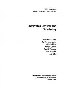
Figure 1 [9].
dx1 (t) dt dx2 (t) dt dx3 (t) dt dx4 (t) dt
Pump 2
u2
The quadruple-tank laboratory process. From
a1 p 2g x1 (t) + A1 a2 p =− 2g x2 (t) + A2 p a = − 3 2g x3 (t) + A3 a p = − 4 2g x4 (t) + A4
=−
a3 p γ 1 k1 2g x3 (t) + u1 (t) A1 A1 a4 p γ 2 k2 2g x4 (t) + u (t) A2 A2 2 (1 − γ 2 )k2 u2 (t) A3 (1 − γ 1 )k1 u1 (t) A4
y1 (t) = kc x1 (t) y2 (t) = kc x2 (t)
where xi is the level, Ai is the cross-section, and ai is the outlet hole cross-section of tank i. The process is linearized around a stationary point, and then sampled with the interval h = 1 s. This gives a standard discrete time state-space model of the process to be used as the internal model by the MPC controller. In the following y1e , y2e , u1e , and u2e denote deviations from the equilibrium point. 2.1 MPC Formulation
2. An MPC Controller An MPC controller for a quadruple-tank process [9] will be described. The tank set-up is shown in Figure 1, and the goal is to control the level of the two lower tanks, y1 and y2 , using the two pumps, u1 and u2 . The flow from pump 1 is divided such that a fraction γ 1 enters tank 1 and 1 − γ 1 enters tank 4. Likewise, the flow from pump 2 is divided such that a fraction γ 2 enters tank 2 and 1 −γ 2 enters tank 3. A nonlinear model of the process is given by
A standard receding horizon MPC formulation based on [11] is used. The function to minimize at time k is V (k) =
Hp X i=1
i yˆ (k + ihk) − r(k + i)i2Q +
HX u −1 i=0
i∆ uˆ (k + ihk)i2R (1)
where yˆ is the predicted output, r is the current level set-point, uˆ is the predicted control signal, H p is the prediction horizon, Hu is the control horizon, Q and R are weighting matrices, and ∆ u( k) = u( k) − u( k − 1). It is assumed that Hu < H p and that uˆ ( k + i) = uˆ ( k + Hu − 1) for i ≥ Hu . Together with constraints on the control signals, u ie ≤ u ie ≤ u¯ie , this ¯ formulation leads to a convex linear-inequality constrained quadratic programming problem (LICQP)
Ideal case Complete optimization in every sample Enforced deadlines by termination Dynamic stop criterion
2
Tank level, ye
1
Tank level, ye
3 2.5 2 1.5 1 0.5 0 −0.5 10
20
30
40
50
60
70
80
90
0 −0.2 −0.4 −0.6 −0.8 −1
100
0
10
20
30
40
50
60
70
80
90
100
0
10
20
30
40
50
60
70
80
90
100
2
Control input, ue
1
Control input, ue
0
0.2
4
2
0
−2 0
10
20
30
40
50
60
70
80
90
100
Time [s]
4
2
0
−2
Time [s]
Figure 2 Comparison of control performance in the single MPC case for different implementations. The solid curve shows the ideal control performance with full optimization and zero execution time. If the computational time is accounted for the performance degrades (dashed). By prematurely aborting the optimization the control performance may improve. However, too early abortion (dotted) gives really bad performance. Best performance is obtained by a dynamic stop criterion (dash-dotted), exploiting the trade-off between delay and continued optimization. The horizontal dotted lines in the control signal plots show the saturation limits.
to be solved each sample. The problem can be written in matrix form as ∆U
subject to
Ω∆U ≤ ω .
2.5
Exec. time [s]
min V ( k) = ∆U T H ∆U − ∆U T G
3
2 1.5 1 0.5
In accordance with the receding horizon principle, only the first element in the control trajectory is applied to the process. In the next sample, new measurements are available and the optimization procedure is repeated.
0
0
20
40
60
80
100
Time [s]
Figure 3 Execution time measurement for the MPC algorithm in the specific simulation scenario given by Figure 2.
2.2 Real-Time Properties Throughout the examples given below, the simulation scenario will be the one shown in Figure 2. At time t = 30 s, a step reference change is commanded in y1e . At the same time a step load disturbance enters in y2e . The reference value for y2e is zero throughout the simulation. The result of an ideal simulation is shown by the solid curves. The control performance is optimal and is obtained by letting the optimization algorithm run to termination in each sample and setting the computational delay to zero in the simulation. A Java-implementation of the MPC controller was used to measure the execution time in the described simulation scenario. The result is shown in Figure 3. A considerable difference in execution time can be noticed between different operating conditions. During steady-state operation the required computation time is negligible, whereas during the transient it
may become well above the period of the controller. The execution time variations depend on a number of factors: the state of the plant, the current and future reference values, the disturbances acting on the plant, the number of active constraints on control signals and outputs, etc. Based on this measurements, the execution time for each iteration of the optimization algorithm in the following simulations was set to 40 ms. Figure 4 shows a close-up of how the objective function (1) decreases for each iteration during one of the samples when the execution time is long. The predicted cost decreases with each new iteration of the QP-solver, but it is also expected that the true control performance will gradually degrade because of the additional delay (indicated by the dotted curve). If the time required to search for a proper control signal sequence is too long, control
900 800 700
value of objective function Cost, V(34)
600 500 400 300
delay−induced cost
200 100 0 33.5
34
34.5
35
35.5
36
36.5
Time [s]
Figure 4 The solid curve shows a close-up of how the objective function (1) decreases for each iteration during a sample when the execution time is long. It is seen that the required execution time for full optimization is well above the period of one second.
performance may actually improve by prematurely terminating the optimization in order to reduce the delay. The QP-solver uses an active set method, and it can be seen that the cost function decreases monotonically but not smoothly by each iteration as the number of active constraints changes. A further discussion regarding proper choices of QP-solvers is given in Section 4.1.
3. Examples of Dynamic Scheduling The following simulation examples will involve two separate cases; first the case of a single MPC controller and then the case where two MPC controllers are competing for computing resources on the same CPU. The MATLAB/Simulink-based simulator TRUETIME [8] is used to simulate controller task execution in a real-time kernel in parallel with the continuoustime dynamics of the quadruple-tank processes. The detailed co-simulation makes it possible to study the effect of different scheduling policies and execution scenarios on the control performance. 3.1 A Single Quadruple-tank Controller The MPC task is implemented using a standard task model, where the task is released periodically and a new instance may not start to execute until the previous instance has completed. The sampling is performed within a separate high-priority task, and the control signal is actuated as soon as the task has completed. In a first attempt, the optimization algorithm is allowed to run to termination in each instance. Because of the execution time characteristics, there will be considerable output jitter and delays. The
result is degraded control performance, as shown by the dashed curves in Figure 2. An obvious alternative would be to terminate the optimization at the end of the period. In this example, however, this turns out to render even worse performance, as shown by the dotted curves in Figure 2. Obviously, the optimization is sometimes terminated too early in this case. In a third attempt, a dynamic stop criterion is used, where the optimization is terminated if it has not finished within two periods. The value of the delay limit was found by extensive simulations. The result is better performance, as shown by the dashdotted curve in Figure 2. The simulations indicate that dynamic scheduling, where the MPC controller is sometimes allowed to miss a deadline, can give better results than terminating the optimization at the deadline or allowing the task to run to completion. 3.2 Two Quadruple-tank Controllers Now consider scheduling of two MPC controllers for two identical quadruple tank processes on the same CPU. Both controllers are designed with the same control and prediction horizons, sampling intervals and weighting matrices. This makes it straightforward to compare the values of the respective cost functions. The simulation scenario for the first MPC controller is the same as before, whereas the reference change and step load disturbance occur ten seconds later for the second MPC controller. The solid curves in Figure 5 show the result of an ideal simulation, with full optimization, no interference and the execution times set to zero. Traditional Scheduling The two MPC controller tasks are first scheduled using standard fixedpriority scheduling. The tasks are implemented as two separate periodic tasks, with MPC 2 given the highest priority. No termination of the optimization algorithms is performed in this simulation. In addition to the delays caused by the long execution times, MPC 1 will now also experience delay due to preemption from the high-priority task, as seen in the computer schedule in Figure 6. The results are given by the dashed curves in Figure 5, and the control performance for MPC 1 is poor. As a comparison the tasks are also scheduled using earliest deadline first (EDF) scheduling [10], where the task with the shortest remaining time to its deadline will be given highest priority. This scheduling policy gives a more fair distribution of the computing resources, and the somewhat improved control performance is shown by the dotted curves in Figure 5.
Ideal case Fixed priority scheduling EDF scheduling Feedback scheduling
Quadruple−tank 1 e
0.1
Tank level, y2
Tank level, y
e 1
4
3
2
1
0
−0.1
−0.2
0 0
10
20
30
40
50
60
70
80
90
0
100
10
20
30
40
50
60
70
80
90
100
10
20
30
40
50
60
70
80
90
100
Quadruple−tank 2 e
0.1
Tank level, y2
e
Tank level, y1
4
3
2
1
0 0
10
20
30
40
50
60
70
80
90
0
−0.1
−0.2
100
0
Time [s]
Time [s]
Figure 5 Scheduling two MPC tasks for two identical quadruple-tank processes. The solid curve shows the optimal performance, corresponding to full optimization, no interference and zero execution times. The other curves show a comparison of control performance obtained by fixed-priority scheduling (dashed), EDF scheduling (dotted), and feedback scheduling (dash-dotted). The introduction of the feedback scheduler, using feedback from the cost functions, improves the control performance considerably.
Computer schedule FP (high=running, medium=preempted, low=sleeping)
let task i perform one iteration; if (optimum_i) { actuate plant; }
MPC 2
}
MPC 1
30
35
40
45
Time [s]
50
55
60
Figure 6 Close-up of the schedule under fixed-priority scheduling. The low-priority controller task (MPC 1) is preempted during significant amounts of time with resulting poor control performance.
Feedback Scheduling The main problem with traditional scheduling approaches is that the (possibly dynamic) priorities of the MPC tasks do not reflect their computational demand nor their relative importance at each point in time. In order to improve the control performance further a feedback scheduler is introduced, which uses the current values of the cost functions to dynamically schedule the MPC tasks. The pseudo-code for the feedback scheduler looks like this:
To guarantee at least nominal stability of the controllers, a controller which does not have a feasible solution yet is associated with an infinite cost (this is typically achieved within the first iteration). The sampling is performed within a separate highpriority task, and when an MPC task has just received new samples, it is also associated with an infinite cost. This ensures that the cost function will become properly updated as soon as possible to reflect current situation in the controlled process. Simulation results using the proposed scheme are given by the dash-dotted curves in Figure 5. It can be seen that the control performance has improved, especially for MPC controller 1. A close-up of the distribution of computing resources in the sample between 44 and 45 seconds is shown in Figure 7. Here it is seen how the execution is divided between the MPC tasks on a per-iteration basis. In the simulation, one scheduling decision is assumed to take 1 ms.
4. Discussion do forever { for (each active MPC task i) { if (delay_i > MAXDELAY_i) { abort optimization; actuate plant; } } determine MPC task i with highest cost;
The simulation results indicate that dynamic scheduling based on feedback from cost functions may be a successful way of dealing with the problem of limited computational time when implementing MPCs. However, to be able to apply the suggested scheme in a more general setting several issues have
Computer schedule (high=running, low=waiting) Feedback Scheduler
MPC 2 Optimization aborted
MPC 1
44
44.2
44.4
44.6
Time [s]
44.8
45
Figure 7 Close-up of the schedule under feedback scheduling. The feedback scheduler distributes the computing resources on a per-iteration basis based on feedback from the cost functions. When the delay exceeds a certain limit the optimization is aborted.
to be addressed. 4.1 Choice of QP-Solver There exist two major families of methods for solving LICQP, see, e.g., [11]. The traditionally most used is the Active Set method, which was used in the examples in this paper. In this algorithm an active set, the set of active inequality constraints, is introduced. At each iteration a solution to a linear-equality constrained quadratic programming problem (LECQP) is obtained. As the algorithm proceeds, constraints are added and removed from the active set until the optimal solution is found. A drawback with this method, as seen in Figure 4, is that the cost function decreases very irregularly which makes it difficult to know how close the optimum is and whether it will pay off to optimize further. In recent years Interior Point methods have won widespread use as an alternative to active set methods. Interior point methods usually maintain a strictly feasible solution at each iteration, see, e.g., [14]. Interior point methods may also be more suitable in a dynamic setting, in that the cost typically decreases more smoothly by each iteration. It is then easier to estimate how much it will pay off to optimize further—the scheduler could look at the time derivatives of the cost functions to decide which MPC controller that should run. A particularly attractive method in the interior point category is the primal-dual interior point method. For convex optimization problems, the algorithm computes the duality gap exactly at each iteration. This is a useful feature, since it gives an indication of how close to the optimal point the solution at hand is, and may be used to decide whether to terminate the algorithm or not. This could be a better indication to the scheduler of what MPC controller that needs attention than just looking at the current cost. As described above, premature termination of an
optimization run in one MPC controller may be justified in order to improve the overall control performance. Given that the algorithm at hand has found a feasible solution (this is considered as a requirement), any of the LICQP algorithms may be terminated before the optimum is found. The quality of the solution then depends on how close to the optimum the solution is. Potentially, this means that the primal-dual interior-point method is preferable, since it offers an estimation of how far off from the optimal value a solution at a given iteration is. It is also expected that the variations in execution time would be less using an interior point method, see, e.g., [2]. 4.2 Computational Delay In the MPC formulation used in this paper the computational delay was not accounted for. Standard practice is to include a one-sample delay in the process description and then synchronize the writing of the outputs with the reading of the inputs to enforce this. The computational delay, however, could vary from a very small fraction of the sampling interval up to several sampling intervals. Compensating for the maximum delay may become very pessimistic and lead to decreased obtainable performance. In the dynamic schemes presented in the paper, the control signal was actuated as soon as the optimization terminated, not to induce any unnecessary delay that degrades the performance. Ideally, this should be combined with an adjustment of the prediction matrices in the next sample according to the actual delay. 4.3 Comparing Cost Functions When scheduling several MPC controllers, the strategy suggested in this paper was to give priority to the controller with the highest current value of its cost function. However, comparing cost functions directly may not be appropriate when the controllers have different sampling intervals, prediction horizons, magnitude of disturbances, etc. In those cases, it would be necessary to scale the cost functions to obtain a fair comparison. The scheduling could also use feedback from the derivatives of the cost functions, as well as the relative deadlines of the different controllers.
5. Conclusions The paper has discussed dynamic scheduling of model predictive controllers. The trade-off between optimization and input-output delay was investigated, and it was shown that early termination of the optimization algorithm can improve overall control performance when computing resources are scarce. In the multi-MPC case a feedback scheduling scheme
was introduced, where computing resources were distributed based on feedback from cost functions. The potential of the suggested scheme was illustrated by simulations, and a number of future research directions were discussed. 5.1 Acknowledgements The work has been supported by LUCAS — the VINNOVA-funded Center for Applied Software Research, and by ARTES — the Swedish Network for Real-time Research and Education.
References [1] K.-E. Årzén, A. Cervin, J. Eker, and L. Sha. “An introduction to control and scheduling co-design.” In Proceedings of the 39th IEEE Conference on Decision and Control, Sydney, Australia, December 2000. [2] R. A. Bartlett, A. Wächter, and L. T. Biegler. “Active set vs. interior point strategies for model predictive control.” In Proceedings of the American Control Conference, Chicago, Illinois, Juny 2000. [3] G. C. Buttazzo. Hard Real-Time Computing Systems: Predictable Scheduling Algorithms and Applications. Kluwer Academic Publishers, 1997. [4] M. Cannon, B. Kouvaritakis, and J. A. Rossiter. “Efficient active set optimization in triple mode MPC.” IEEE Transactions on Automatic Control, 46:8, pp. 1307–1312, August 2001. [5] A. Cervin, J. Eker, B. Bernhardsson, and K.-E. Årzén. “Feedback-feedforward scheduling of control tasks.” Real-Time Systems, 23, pp. 25–53, 2002. [6] W. B. Dunbar, M. B. William, R. Franz, and R. M. Murray. “Model predictive control of a thrust-vectored flight control experiment.” In Proceedings of the 15th IFAC World Congress on Automatic Control, Barcelona, Spain, July 2002. [7] C. E. Garcia, D. M. Prett, and M. Morari. “Model predictive control: Theory and practice – a survey.” Automatica, 25:3, pp. 335–348, 1989. [8] D. Henriksson, A. Cervin, and K.-E. Årzén. “Truetime: Simulation of control loops under shared computer resources.” In Proceedings of the 15th IFAC World Congress on Automatic Control, Barcelona, Spain, July 2002. [9] K. H. Johansson. “The quadruple-tank process: A multivariable process with an adjustable zero.” IEEE Transactions on Control Systems Technology, 8:3, May 2000. [10] J. W. S. Liu. Real-Time Systems. Prentice-Hall, 2000. [11] J. M. Maciejowski. Predictive Control with Constraints. Prentice-Hall, 2002. [12] J. Richalet. “Industrial application of model based predictive control.” Automatica, 29, pp. 1251–1274, 1993.
[13] P. O. M. Stokaert, D. Q. Mayne, and J. B. Rawlings. “Suboptimal model predictive control (feasibility implies stability).” IEEE Transactions on Automatic Control, 44:3, pp. 648–654, March 1999. [14] S. J. Wright. Primal-Dual Interior-Point Methods. SIAM, 1997.