Dynamic Skyline Queries in Large Graphs 3 ¨ Lei Zou1 , Lei Chen2 , M. Tamer Ozsu , and Dongyan Zhao1,4 1
4
?
Institute of Computer Science and Technology, Peking University, Beijing, China, {zoulei,zdy}@icst.pku.edu.cn 2 Hong Kong of Science and Technology, Hong Kong, China,
[email protected] 3 University of Waterloo, Waterloo, Canada,
[email protected] Key Laboratory of Computational Linguistics (PKU), Ministry of Education, China Abstract. Given a set of query points, a dynamic skyline query reports all data points that are not dominated by other data points according to the distances between data points and query points. In this paper, we study dynamic skyline queries in a large graph (DSG-query for short). Although dynamic skylines have been studied in Euclidean space [16], road network [6], and metric space [4, 7], there is no previous work on dynamic skylines over large graphs. We employ a filter-and-refine framework to speed up the query processing that can answer DSG-query efficiently. We propose a novel pruning rule based on graph properties to derive the candidates for DSG-query, that are guaranteed not to introduce false negatives. In the refinement step, with a carefully-designed index structure, we compute short path distances between vertices in O(H), where H is the number of maximal hops between any two vertices. Extensive experiments demonstrate that our methods outperform existing algorithms by orders of magnitude.
1 Introduction As a popular multi-criteria decision making and business planning operator, skyline has attracted considerable attention. Given a record set D of n dimensions, a skyline query over D returns a set of records that are not dominated by any other record in D [2]. A record r is said to dominate another record r0 , if and only if the value of r is no larger than that of r0 in each dimension, and the value of r is smaller than that of r0 in at least one dimension. Fig. 1 shows a simple skyline query example. Given a record set D with 8 records, only 001 and 003 are reported as skyline records, since they are not dominated by any other record in D. The others are all dominated by 001 or 003. For example, 002 is dominated by 001, since 2 < 3 in dimension x and 3 < 4 in dimension y. Based on the skyline definition, given a record set D, the skylines of D are fixed, thus, we refer to the skylines following the original definition as static skylines [4]. In some cases, the values of records are computed at run time based on the values of query points, even for the same record set D, given different query points, we might obtain different skylines. We refer to these as dynamic skylines. These have been studied in various contexts. For example, “spatial” skylines have been proposed in Euclidean ?
Lei Zou and Dongyan Zhao were supported by the National High Technology Research and Development Program(“863”Program) of China (No. 2009AA01Z408). Lei Chen was supported by NSFC/RGC joint research scheme under project no. N HKUST612/09. M. Tamer ¨ Ozsu’s research has been supported by Natural Sciences and Engineering Research Council (NSERC) of Canada.
2
Lei Zou et al.
space [16]. Specifically, given a set of query points Q = {qi } (i = 1...n), for each record r ∈ D, we compute a new vector rd of dimension n, where rd ’s i-th dimension is computed as Euclidean Distance between r and qi . The spatial skylines refer to all vectors rd whose values are not dominated by other r0d in the record set D. A similar query, called multi-source skyline query in road networks, is studied by Deng et al. [6], where the values of records are defined as the shortest path lengths on road networks from data points to query points.
Y 8
Record Set D 005
7
006
6 004 5
00 2
4
007 008
001
3
006
2 1
003 Skyline Records 1
2
3
4
5
6
7
8 X
(a) Static Skylines
v1 q1
v0
ID
X
Y
001
2
3
002
3
4
003
4
2
004
4
5
005
6
7
ID
006
6
3
007
7
6
v0 v3 v4
008
5
4
v4
v3
v2 q2
Dist (vi , q1 ) Dist(vi , q2 ) 1 2 3
1 1 2
(b) Running Example
Fig. 1. (a)Static Skyline Query and (b) Running Example
Compared to static skylines, dynamic skylines offer users more flexibility in specifying their search criteria. In other words, different users can specify different sets of query points. Meanwhile, the flexibility of dynamic skyline queries brings new challenges for efficient query processing. A naive solution computes all the new vectors according to the query points, and then searches the skylines over the generated vectors. This approach is clearly inefficient, since it requires scanning the whole record set D to compute the new vectors. In this paper, we study the problem of dynamic skyline queries over graph data, which is formally defined as follows: Definition 1. Dominate. Given a large undirected and edge-weighted graph G and a set of query vertices Q = {qi }, i = 1...n, in graph G, for two data vertices v 0 and v in G (v and v 0 are not query vertices), we say that v 0 dominates v, if and only if the following holds: (∀i, Dist(v 0 , qi ) ≤ Dist(v, qi )) ∧ (∃j, Dist(v 0 , qj ) < Dist(v, qj ) , where Dist(v, qi ) is the shortest path distance between v and qi in graph G. Definition 2. Problem Definition. Given a large undirected and edge-weighted graph G and a set Q of query vertices Q = {qi }, i = 1...n, in graph G, a dynamic skyline query in graph (DSG-query) reports all data vertices v in graph G (v 6= qi ) where each v is not dominated by any other vertex v 0 in G. All skyline vertices of query Q in graph G are denoted as Skyline(G, Q). Example 1 (Running Example). Consider a graph G and two query vertices q1 and q2 (denoted as shaded vertices) in Fig. 1b. The number in the vertex is the vertex ID. For simplicity, we assume that all edges have the same weight 1. Obviously, in this example, there is only one skyline vertex, that is v0 . Similar to the cases in the Euclidean space, dynamic skylines over graph data are quite useful. For example, given a social network modeled as a large graph, where each vertex corresponds to an individual, and each edge denotes the friendship between two corresponding individuals, we can use shortest path distance to define the relationship
Dynamic Skyline Queries in Large Graphs
3
score between two individuals in a social network [18]. Assuming that there are two important latent customers (two query vertices), a company may look for a salesman who has “closer” relationship to these customers than any other salesmen. In fact, the company is looking for the skyline salesmen with respect to the two given potential customers c1 and c2 . A salesman r is a skyline if and only if there exists no other salesman r0 , such that Dist(r0 , c1 ) < Dist(r, c1 ) and Dist(r0 , c2 ) < Dist(r, c2 ), where Dist(r, ci ) denotes the shortest path distance between r and ci . Finally, consider a Peer-to-Peer (P2P) network with a number of peers that are interested in some movies. In order to reduce the communication cost, we can put replicas of the movies on a node that is near these peers. Obviously, dynamic skylines with respect to these peers in the topology map (a graph) of this P2P network can provide some candidate nodes for storing the replicas. Although efficient solutions have been proposed for dynamic skylines over Euclidean space [16], these cannot be applied to graphs. In a graph, the shortest path distance is often used as a measure between two vertices, rather than Euclidean distance. Thus, it is impossible to utilize existing pruning rules, such as MBR and Voronoi Diagrams that have been used in Euclidean space [16]. The most related work is multi-source skyline query processing in road networks [6], which also uses shortest path distance as the measure. Three different algorithms have been proposed to find dynamic skylines in road networks. Two of the algorithms (EDC and LBC) [6] utilize Euclidean distance as the lower bound of shortest path distance in a road network to perform pruning. However, for a general graph G, we cannot define Euclidean distances to bound the shortest path distances between any two vertices in G, since there is no coordinate associated with each vertex. Therefore, EDC and LBC algorithms cannot be applied to DSG-Query. The third algorithm (CE) is not efficient. It expands each query point towards all directions, which may generate too many candidate objects and cause unnecessary shortest path distance computation, as confirmed by our experiments (Section 4). Dist(v, qi ) in DSG-query is a metric distance. Thus, the approaches that address skyline queries in metric space (e.g. [4]) are of interest. However, these solutions are only designed for the general metric space, and the methods are not optimized for large graphs. Experiments in Section 4 show that our methods outperform these general approaches by orders of magnitude. For a DSG-query, there exist two challenges: 1) Huge Search Space: each vertex in graph G (except for query vertices) is a candidate for DSG-query; and 2) Expensive Shortest Path Computation: In order to find final skyline vertices, we need to compute Dist(v, qi ) (see Definitions 1 and 2). However, the expansion process in shortest path algorithms (e.g. Dijkstra’s Algorithm [5]) is very time-consuming, especially in very large graphs. In order to address the above challenges, we adopt the “filter-and-refine” framework. During the filtering process, we prune most false positives (the vertices that cannot be skyline vertices) to generate a set of candidate vertices. We compute Dist(v, qi ) for each candidate vertex during refinement using an index structure. Furthermore, we can compute Dist(v, qi ) in O(H)where His the number of maximal hops between any two vertices in the graph, without expensive expansions that are employed in previous solutions. In summary, we make the following contributions:
4
Lei Zou et al. 1. We propose shared-shortest-paths (SSP) pruning for DSG-query, that considers graph properties, and that filters out most false positive vertices. We also give a theoretical analysis of the pruning power of SSP-pruning. 2. During offline processing of DSG-query, we build carefully-designed index structures that support both filtering and verification processes in online DSG-query. 3. Based on novel pruning rules and index structures, we propose the SSP query algorithm (see Algorithm 3) for DSG-query. 4. We show by extensive experiments that our methods have good pruning power and fast query response time.
The remainder of this paper is organized as follows. Some background knowledge is discussed in Section 2. A novel pruning rule is proposed in Section 3. The index structures and SSP-query algorithm are also presented in Section 3. We evaluate the efficiency of our methods with extensive experiments in Section 4. We discuss related work in Section 5 in detail. Finally, we conclude the paper in Section 6.
2 Preliminaries Definition 3. Shortest Path Tree. (SP -Tree for short) Given a large graph G and a vertex v, we perform a single-source shortest path algorithm (such as Dijkstra algorithm [5]) from vertex v to get a tree SP (v). The root of SP (v) is v, and all paths from v to another node v 0 in SP (v) is the shortest path from v to v 0 in graph G.
SP(v1)
SP(v0)
v1
SP(v2)
v1
v0
v2
v3
v4
v0
SP(v3)
v2
v0
v1
SP(v4) v4
v3
v2
v3
v3
v2
v4
v3 v4
v0
v4
v2
v1 v0
v1
Fig. 2. Shortest Path Trees Fig. 2 shows all SP -Trees for graph G of Example 1. We can perform Dijkstra’s algorithm [5] offline to obtain the SP -Tree. Note that, for a vertex v in a large graph G, there may exist more than one SP -Tree rooted at v. Actually, for a vertex v in G, we can select any SP -Tree rooted at v without affecting the correctness of our methods. We will prove this claim in Section 3 (see Lemma 4). We utilize SP-Tree in our SSP query algorithm (see Section 3). Definition 4. Minimum Common Ancestor. Given a SP -Tree SP (v) in a large graph G and a set of nodes {v1 , ..., vn } in SP (v), a node v 0 is the minimum common ancestor of {v1 , ..., vn } (denoted as M CA(v1 ...vn , SP (v))) if and only if 1) v 0 is the ancestor of all nodes v1 , ..., vn ; and 2) there exists no other node v 00 , where v 00 is the ancestor of all nodes v1 , ..., vn , and v 0 is the ancestor of v 00 . Take SP (v3 ) in Fig. 2, for example, M CA(v0 , v1 , SP (v3 )) = v2 .
3 Shared Shortest Path Algorithm 3.1 SSP Pruning Algorithm We first note an interesting property of graphs: many pairwise shortest paths in a graph have shared parts. We propose a pruning strategy (SSP Pruning) that exploits these
Dynamic Skyline Queries in Large Graphs SP(V4)
V0
V4
to be pruned
q1 ĂĂ
SP(V0)
v'
v
V1
V2
q1
qn
5
V3 q2
V3
V2
V4 (a)
V0
q2
V1
q1
(b)
Fig. 3. (a)Shared Shortest Path Pruning and (b) Lemma 2
shared paths. We also give a theoretical analysis of pruning power of SSP pruning. Theoretical analysis and experiments confirm the effectiveness of SSP pruning. Furthermore, the indexing structures proposed for SSP can be used to support the efficient computation of Dist(v, qi ) (discussed in Section 3.2). Pruning Rule 1: Shared Shortest Path (SSP) Pruning. Given a large graph G and a set of query vertices Q = {qi }, i = 1...n, for a data vertex v, if there exists at least one joint (common) vertex v 0 among all shortest paths between v and qi (denoted as vqi )(v 6= v 0 , i = 1...n), v can be pruned safely for DSG-query. Lemma 1. SSP pruning will not lead to false negatives. Proof. Since vertex v 0 is in the shortest path vqi (as shown in Fig. 3a), it is straightforward to see that Dist(v 0 , qi ) < Dist(v, qi ), i = 1...n . According to Definition 1, vertex v 0 dominates v. Therefore, v cannot be a skyline vertex, without causing false negatives. Definition 5. Strictly Dominate, Candidate Skyline Vertex. Given a large graph G and a set Q of query vertices Q = {qi }, i = 1...n, for a vertex v, if there exists a joint vertex v 0 (v 6= v 0 ) in all shortest paths vqi , vertex v 0 strictly dominates vertex v. For a vertex v in graph G, if there exists no other vertex v 0 that strictly dominates v, the vertex v is a candidate skyline vertex. Theorem 1. Given a large graph G and a set Q of query vertices Q = {qi }, i = 1...n, the following formula holds:Skyline(G, Q) ⊆ Can Skyline(G, Q), where Skyline(G) (or CanSkyline(G)) is the set of skyline vertices (or candidate skyline vertices) in graph G. Proof. SSP-pruning will not lead to false negatives, therefore, Skyline(G, Q) ⊆ Can Skyline(G, Q) Obviously, CanSkyline(G, Q) can be regarded as a candidate set for Skyline(G, Q). In Example 1, we enumerate all SP -Trees in graph G, as shown in Fig. 2. Lemma 2. Given a large graph G, a set Q of query vertices Q = {qi }, i = 1...n, and a SP -Tree SP (v) and v 0 = M CA( q1 ...qn , SP (v)), v is a candidate skyline vertex if and only if v = v 0 . Proof. Proof is based on Definition 5. Due to space limit, we omit the details. We show two shortest path trees SP (v0 ) and SP (v4 ) in Fig. 3b. In these trees, M CA(q1 , q2 , SP (v4 )) = v3 6= v4 , therefore,v4 ∈ / CanSkyline(G, Q). However, M CA(q1 , q2 , SP (v0 )) = v0 , thus, v0 ∈ CanSkyline(G, Q).
6
Lei Zou et al.
Using Lemma 2, we propose a conceptually simple framework for SSP-pruning. During offline processing, we enumerate all SP -Trees in graph G. Given a set Q of query vertices Q = {qi }, i = 1...n, in each SP (v), if v 0 = M CA(q1 ... qn , SP (v)) and v 0 = v , v will be inserted into candidate set CL. Otherwise, v can be pruned safely. We can find CanSkyline(G, Q) by sequentially scanning all SP -Trees. However, due to large space cost, it is impractical to store all SP -Trees of a large graph G. The space cost of each SP -Tree is O(|V (G)|), where |V (G)| is the number of vertices in G. Therefore, we would need O(|V (G)|2 ) space to store all SP -Trees in graph G. For example, if G has 10K vertices, the total space cost is O(108 ). To alleviate this space cost, in this work, we only store 1-hop SP -Trees. Definition 6. 1−Hop Shortest Path Tree Given a large graph G and a vertex v in G, 1Hop Shortest Path Tree from v (denoted as SP (v, 1)) is obtained by extracting vertex v and vertices that are directly reachable from v in SP (v). Each leaf node f in SP (v, 1) also has a set des of vertices (denoted as f.des), that corresponds to all descendants of the leaf node f in SP (v). We call f.des the node area of f .
SP(v0) v0 v1 v1.des =
v2 v2.des = {v3,v4}
Fig. 4. 1−Hop Shortest-Distance-Path Tree
Fig. 4 shows SP (v0 , 1) in Example 1, that is obtained by extracting vertices v1 and v2 that are directly reachable from v0 in SP (v0 ) to form SP (v0 , 1). Since vertices v3 and v4 are descendants of v2 in SP (v0 ), v2 .des = {v3 , v4 }. Theorem 2. Given a set of query vertices Q = {qi }, i = 1...n, and 1-hop SP-Tree SP (v, 1), if there exists a leaf node f in SP (v, 1) and f.des contains all query vertices, vertex v cannot be a skyline vertex. Proof. Proof is based on Definition 5. Due to space limit, we omit the details. Based on Theorem 2, we propose Algorithm 1. For a vertex v, we only need to check whether all query vertices are in the same leaf node area f.des. If so, v can be pruned. Furthermore, Lemma 3 shows that using 1-hop shortest path tree does not affect the pruning power of Pruning Rule 1. Lemma 3. Given a large graph G and a set of query vertices Q = {qi }, i = 1...n, for a data vertex v in G, if v is strictly dominated by another vertex v 0 , then there must exist a leaf node f in SP (v, 1) and f.des contains all query vertices. Proof. Since v 0 strictly dominates v, all query vertices are descendent of v 0 in SP (v). According to Definition 6, it is straightforward to know all query vertices are in one leaf node area f.des.
Dynamic Skyline Queries in Large Graphs
7
Algorithm 1 Prune False Positives by SSP pruning SSP-pruning(G,Q,S) Require: Input: A large graph G and a set Q of query vertices Q = {qi }, all 1-hop SP Trees, and a set S of vertices Output: Candidate Set CL 1: for each vertex v in S do 2: if all query vertices qi are in only one leaf node n.des of SP (v, 1) then 3: continue (Pruned by Theorem 2 ) 4: else 5: insert v into candidate set CL. 6: report CL
Lemma 4. Given a vertex v that has more than one SP -Tree rooted at v (SP1 (v), ..., SPb (v)), choosing any SP-Tree rooted at v for SSP pruning does not lead to false negatives. Proof. No matter which SPj (v) is selected, if all query vertices are contained in f.des of SPj (v), f strictly dominates v. Therefore, Lemma 4 holds. However, the space cost of the set f.des in each leaf node f is still a problem. The number of vertices in f.des is always large. In order to reduce the space cost, we build hierarchical clusters on vertices in G. If f.des contains all vertices in a cluster P , we can use P 0 s ID instead of the vertices in P in f.des. For example, Fig. 5a shows a hierarchical cluster of Example 1. Cluster P2 has two vertices: v3 and v4 . Fig. 5b shows that v3 and v4 are both in v2 .des of SP (v0 , 1). Therefore, we only need to insert P2 instead of v3 and v4 in v2 .des of SP (v0 , 1), as shown in Fig. 5c. Intuitively, if some vertices often occur together in f.des, they should be grouped together. Based on this intuition, we propose distance definitions (Definitions 7 and 8) that account for clustered vertices. In Example 1, vertices v3 and v4 should be grouped into one cluster, since they occur together in three 1-hop SP -Trees (i.e. SP (v0 , 1), SP (v1 , 1) and SP (v2 , 1)). Similarly, v1 and v2 should be clustered together. Essentially, the coherence of vertices in 1-hop SP-Tree is derived from their shared shortest paths of SP -Trees. P
SP(v0,1) P0
P1
SP(v0,1)
P2
v0
v1
v2
v3
Hierachical Cluster Tree (a)
v4
v1
v2 v2.Des={v3,v4} (b)
v1
TAB_1SPT dst P2 ...
v0
v0
src v0 ...
lef v2 ...
v2 v2.Des={P2} (c)
(d)
Fig. 5. Hierarchical Cluster Tree and 1-Hop SP -Tree
In order to build a hierarchical cluster on vertices, we propose the following distance functions, which are used to measure the probability that two vertices appear together. Definition 7. Vertex Distance. Given three vertices v, v1 and v2 , if there exists a leaf node f in SP (v, 1) and f.des contains both v1 and v2 , we say that v1 and v2 occur together in SP (v, 1). Let the number of vertices v in which v1 and v2 occur together in
8
Lei Zou et al.
SP (v, 1) be T . Then, vertex distance between v1 and v2 (denoted as V exDis(v1 , v2 )) is defined as: T V exDis(v1 , v2 ) = |V (G)| Definition 8. Cluster Distance. Given two clusters P1 and P2 and a vertex v, if there exists a leaf node f in SP (v, 1) and f.des contains all vertices in P1 and P2 , we say that P1 and P2 occur together in SP (v, 1). Let the number of vertices v in which P1 and P2 occur together in SP (v, 1) be D. Then, cluster distance between P1 and P2 (denoted as CluDis(P1 , P2 )) is defined as: CluDis(P1 , P2 ) =
D |V (G)|
We employ bottom-up clustering to build the hierarchical clusters. First, based on vertex distances (Definition 7), we utilize clustering algorithms to find clusters on vertices. Then, based on cluster distance (Definition 8), small clusters are grouped into larger ones. We can recursively build a hierarchical cluster tree HT on vertices in graph G, as shown in Fig. 5a. In practice, we store 1-hop SP-Tree in tables using a commercial RDBMS. The table format is shown in Fig. 5d, where ‘dst’ denotes a destination vertex (or a destination cluster),‘src’ denotes a source vertex, and ‘lef ’ denotes that the leaf node f whose node area f.des contains the destination dst in SP (src, 1). We illustrate the methods using Fig. 5. Since the cluster P2 is in v2 .des of SP (v0 , 1), there is a row ‘P2 , v0 , v2 ’ in table T AB 1SP T , which means that v2 .dst contains P2 in SP (v0 , 1). Pruning Power of SSP Pruning We discuss the pruning power of SSP pruning. To facilitate analysis, we assume that all query vertices are selected independently. First, in Lemma 5, we discuss the probability that one vertex v can be pruned in DSG-query with n query vertices. Lemma 5. Given a vertex v in graph G, there are C leaf nodes in SP (v, 1). The number of vertices in each leaf node area fc .des is denoted as |fc .des|, c = 1...C. Given a query set of Q = {qi }, i = 1...n, the probability P r(v) that v is pruned can be evaluated by the following formula. P r(v) =
C X 1 |fi .des|n |V (G)|n i=1
(1)
Proof. If all query vertices are in one leaf node area fc .des of SP (v, 1), fc strictly dominates v ( Definition 5). Therefore, according to Algorithm 1 and SSP pruning, v can be filtered out safely. The probability that one query vertex qi is in node area fc .des is |f|Vc .des| (G)| . Since all query vertices are selected independently, the probability that all n query vertices are in the same node area fc .des is ( |f|Vc .des| (G)| ) . Since there are C leaf nodes in SP (v, 1), we obtain:
P r(v) =
C X 1 |fi .des|n |V (G)|n i=1
Dynamic Skyline Queries in Large Graphs
9
Theorem 3. Given a large graph G with |V (G)| vertices, and a query set of Q = {qi }, i = 1...n, the expected number of pruned vertices can be evaluated by the following formula. |V (G)|
X
P r(vi )
(2)
i=1
where P r(vi ) is evaluated by Equation 1. In the above analysis, we assume that all query vertices are selected independently. We evaluate Equation 2 in experiments (see Section 4) and show that the simple model can provide a good approximation of SSP’s pruning power. 3.2 Computing Shortest Path Distance As stated in Section 1, given a DSG query, we adopt filter-and-refine framework to find the answers. In the refinement phase, in order to avoid the expensive expansion in shortest-path algorithms, we can compute Dist(vj , qi ) directly based on 1-hop SP Trees. The recursive algorithm (DisQ algorithm) shows the computation of Dist(v, q). DisQ is a recursive function. If the destination vertex q is in SP (v, 1), we can report Dist(v, q) directly (Lines 2-3). Otherwise, if the leaf node area f.des in SP (v, 1) contains q, we recursively call DisQ(f, q) to compute Dist(f, q) (Line 5). Finally, we report Dist(v, q) = Dist(v, f ) + Dist(f, q) (Line 6). Algorithm 2 Shortest-Distance Query DisQ(v, q) Require: Input: v and q: two vertices in graph G; SP (v): all 1-Hop SP-Trees Output: Dist(v, q): the shortest distance between the two vertices v and q. 1: if vertex q is a leaf node in SP (v, 1) then 2: Return Dist(v, q) 3: else 4: There is leaf node f in SP (v, 1), and f.des contains q. 5: Call DisQ(f, q) to compute Dist(f, q) 6: Return Dist(v, f )+Dist(f, q).
Theorem 4. The time complexity of DisQ(v, q) Algorithm (see Algorithm 2) in the worst case is O(H), where H is the number of maximal hops between any two vertices in graph G. Proof. Algorithm 2 is a recursive algorithm. Since the number of maximal hops between any two vertices is H, we recursively call DisQ(v, q) at most H times. In each iteration, the time complexity is O(1). Therefore, the time complexity of Algorithm 2 is O(H). 3.3 Putting It All Together: SSP Query Algorithm We propose SSP-query algorithm in Algorithm 3, which calls SSP pruning algorithm (Algorithm 1) to obtain candidates in CL (Line 1). After that, Algorithm 2 is executed to compute Dist(v, q) (Line 4). Skyline vertices are obtained by BNL algorithm [2] (Line 5). Finally, we report the final results RS (Line 6).
10
Lei Zou et al.
Algorithm 3 SSP Query Algorithm Require: Input: G: a large graph; Q: a set of query vertices Q = {qi } Output: RS: the final skyline vertices. 1: call SSP P rune(G, Q) (Algorithm 1) to obtain candidate set CL. 2: for each candidate vertex v in CL do 3: for each query vertex qi do 4: call DisQ(v, q) (Algorithm 2) to compute Dist(v, q). 5: perform BNL algorithm to find skyline vertices, and insert them into answer set RS. 6: Report RS.
4 Experiments In this section, we evaluate our methods over both real data sets and synthetic data sets. Although several efficient dynamic algorithms have been proposed, such as B2 S2 and VS2 [16] in spatial data and EDC and LBC algorithm [6] in road network, they cannot be applied to general graph data as discussed in Section 1. The two algorithms (EDC and LBC algorithms) proposed in [6] are not applicable to a DSG-query, since they employ Euclidean distances as lower bounds of shortest path distances in a road network. There is no coordinate associated with each vertex, thus, it is impossible to employ Euclidean distances as lower bounds of shortest path distances in general graphs. Therefore, we exclude them from comparisons. We compare our methods with MSQ algorithm [4], since MSQ can work on any metric space and the distance function Dist(v, q) in a graph is also a metric function. We also compare our algorithm with CE algorithm [16]. Although CE algorithm is proposed for skyline queries in road networks, it does not utilize special properties of road networks, suggesting that CE can handle dynamic skyline queries in general graphs. CE runs Dijkstra’s algorithm from each query vertex in parallel until that at least one vertex is done by all query vertices. All un-visited vertices can be pruned safely. Furthermore, in the experiments, we also run linear scan for a DSG query as the straightforward approach, denoted as LS algorithm. Specifically, we first perform Dijkstra’s algorithm [5] from each query vertex qi to obtain Dist(v, qi ) for each vertex v in graph G. After that, we perform BNL algorithm [2] to find results from all vertices in graph G. All experiments are implemented using standard C++ and conducted on a P4 1.7GHz machine with 1G RAM running Windows XP. Data Sets: a) S.cerevisiae Dataset: This dataset (http://dip.doe-mbi.ucla.edu) is an undirected graph G in which each vertex represents a protein and each edge represents interactions between two proteins. There are 4934 vertices and 17346 edges in G. In experiments, we set all edge weights to be “1”. b) DBLP Dataset: This dataset is the well-known publication data from DBLP (dblp.unitrier.de/xml/). We construct a co-author network G: every author is denoted as a vertex in G; and an edge is introduced when the corresponding two authors have at least one co-authored paper. We consider 100 important conferences in different areas to construct G. On the whole, there are about 100K vertices and about 400K edges in G. We also set all edge weights to be “1”. c) Synthetic Dataset: We use the graph generator gengraph win ( www.cs.sunysb.edu/ algorith/implement/ viger/distrib/). In experiments, we generate a large graph G with 10K
Dynamic Skyline Queries in Large Graphs
11
vertices satisfying power-law distribution. The edge weights in G satisfy random distribution between [1, 1000]. We denote the synthetic data set as P owerlaw10K. We generate query sets by similar methods to those employed in previous studies [16, 4]. We first randomly choose a vertex o in graph G, then retrieve M ax{λ × |V (G)|, n} vertices in G that are the closest to o, and finally randomly select n vertices from them as query vertices. λ is a parameter within (0,1), |V (G)| is the number of vertices in G, and n is the number of query vertices. Intuitively, large λ leads to a large diameter of query vertices in G. We evaluate query performance under different λ in Section 4. 4
4
10
10
3
SSP MSQ CE AnswerSet
2
10
1
10
Average Candidate Size
Average Candidate Size
Average Candidate Size
10
3
10
SSP MSQ CE AnswerSet
2
10
3
10
2
10
SSP MSQ CE AnswerSet
1
986
1972 2958 3944 The Number of Vertices in Graph G
(a)
10 2000
4934
4000 6000 8000 The Number of Vertices in Graph G
(b)
S.cerevisiae
10000
20K
40K 60K 80K The Number of Vertices in Graph G
(c)
P owerlaw10K
100K
DBLP
Fig. 6. Candidate Size vs. Data Size 4
4000
The Number of Dominance Checks
The Number of Dominance Checks
5000
SSP MSQ CE LS
3000 2000 1000 0 986
1972 2958 3944 The Number of Vertices in Graph G
(a)
x 10
SSP MSQ CE LS
3.5 3 2.5 2 1.5 1 0.5 0 2000
4934
The Number of Dominance Checks
4
6000
4000 6000 8000 The Number of Vertices in Graph G
(b)
S.cerevisiae
5
10
SSP MSQ CE LS
4
10
10000
20K
40K 60K 80K The Number of Vertices in Graph G
(c)
P owerlaw10K
100K
DBLP
−1
10
−2
10
986
SSP MSQ CE LS
1972 2958 3944 The Number of Vertices in Graph G
(a)
S.cerevisiae
4934
Response Time (in Seconds)
Response Time (in Seconds)
Response Time (in Seconds)
Fig. 7. Number of Dominance Checks vs. Data Size
−1
10
−2
SSP MSQ CE LS
10
2000
4000 6000 8000 The Number of Vertices in Graph G
10000
0
10
SSP MSQ CE LS −1
10
20K
(b) P owerlaw10K Fig. 8. Response Time vs. Data Size
40K 60K 80K The Number of Vertices in Graph G
(c)
100K
DBLP
Query Performance vs. Data Sizes In this subsection, we test our algorithm (denoted as SSP) under different data sizes, and compare it with MSQ and LS over both real datasets and synthetic datasets. In this set of experiments, we set n = 5, and λ = 0.003. Fig. 6 shows the pruning power of different methods. SSP has the highest pruning power. Furthermore, the pruning power of SSP is stable in all datasets, and scales well with increasing data sizes. MSQ does not work well, especially in large graphs. This is because the pivots in graph G cannot provide the tight bound for the shortest-path distance Dist(v, q). The candidate size in CE algorithm is larger than that in SSPalgorithm. In CE, we need to expand each query point in ascending order of their shortest path distance to this query point (in parallel). The expansion process stops when
12
Lei Zou et al.
there exists at least one vertex that is visited by all query points. Therefore, as mentioned in [6], CE may result in many candidates and cause unnecessary shortest-path distance computation. Fig. 7 illustrates the number of dominance checks in different methods during DSGquery. With increasing data size, the number of dominance checks also increases in all algorithms. SSP requires fewer dominance checks than other algorithms by orders of magnitude, which again confirms the superior efficiency of SSP. Fig. 8 shows the total response time in different methods. MSQ, CE and LS all need to perform Dijkstra’s algorithm [5] from each query vertex qi . The time complexity of Dijkstra’s algorithm is O(|V (G)|2 ). In CE algorithm, we also need to expand each query vertex by Dijkstra’s algorithm. The cost of running Dijkstra’s algorithm consti1 of tutes the major portion of the response time. Figure 6 shows that |CL| is about 10 |V (G)|. Thus, SSP’s total response time outperforms MSQ, CE and LS by orders of magnitude, as observed in Figure 8. Query Performance vs. Query Size In this set of experiments, we evaluate SSP under different query sizes. Specifically, we set the number of query vertices n = 2, 3, 5, 8, 10, and λ = 0.003. As in traditional skylines, with increasing dimensions (i.e. the number of query vertices), the number of skyline vertices as well as the number of candidates grow. Fig. 9 shows that SSP still has the highest pruning power under different query sizes, consequently, the number of dominance checks is smaller than in other methods (Fig. 10). Figure 11 further shows that the total response time of SSP is the smallest among all methods under various query sizes. 4
10
4
10
SSP MSQ CE AnswerSet
2
10
Average Candidate Size
Average Candidate Size
Average Candidate Size
3
10
3
10
SSP MSQ CE AnswerSet
2
10
3
10
2
10
SSP MSQ CE AnswerSet
1
10
2
3 5 8 The Numer of Query Vertices
(a)
2
10
3 5 8 The Number of Query Vertices
(b)
S.cerevisiae
2
10
3 5 8 The Numer of Query Vertices
(c)
P owerlaw10K
10
DBLP
Fig. 9. Candidate Size vs. Query Size 4
7000 6000
The Number of Dominance Checks
The Number of Dominance Checks
8000
SSP MSQ CE LS
5000 4000 3000 2000 1000 0 2
3 5 8 The Number of Query Vertices
(a)
S.cerevisiae
10
x 10
6 5
6
10 The Number of Dominance Checks
7
9000
SSP MSQ CE LS
4 3 2 1 0 2
3 5 8 The Number of Query Vertices
(b)
P owerlaw10K
10
5
10
4
10
2
SSP MSQ CE LS 3 5 8 The Number of Query Vertices
(c)
10
DBLP
Fig. 10. Number of Dominance Checks vs. Query Size
Query Performance vs. Query Distribution In this subsection, we test SSP under different query vertex distributions. Obviously, large λ means a large diameter of query vertices in G. In this set of experiments, we set λ = 0.001, 0.002, 0.003, 0.004, 0.005,
Dynamic Skyline Queries in Large Graphs 2.5 SSP MSQ CE LS
0.8 0.6 0.4 0.2 0 2
3 5 8 The Number of Query Size
(a)
5
SSP MSQ CE LS
2
Response Time (in Seconds)
1
Response Time (in Seconds)
Response Time (in Seconds)
1.2
1.5 1 0.5 0 2
10
13
3 5 8 The Number of Query Size
SSP MSQ CE LS
4 3 2 1 0 2
10
3 5 8 The Number of Query Size
(b) P owerlaw10K (c) Fig. 11. Total Response Time vs. Query Size
S.cerevisiae
10
DBLP
and the number of query vertices n = 5. Fig. 12 shows that, with increasing query diameter, the cardinality of candidates in SSP also increases. This means that the pruning power of SSP decreases. The reason can be explained as follows: When query diameter is large, the probability that all query vertices are in one node area f.des is small. Actually, MSQ’s and CE’s pruning powers also decrease when query diameter is large. However, the decrease in SSP’s pruning power is smaller than MSQ’s and CE’s, as shown in Fig. 12. Fig. 13 and 14 show that the number of dominance checks and total response times increase with increasing of query diameter in both SSP and MSQ. This can be explained by the decreasing pruning power in Fig. 12. 4
10
4
2
10
SSP MSQ CE AnswerSet
Average Candidate Size
Average Candidate Size
Average Candidate Size
10 3
10
3
10
SSP MSQ CE AnswerSet 2
0.002
(a)
0.003 λ
0.004
0.001
0.005
SSP MSQ CE AnswerSet 2
10
0.001
3
10
0.002
0.003 λ
0.004
10 0.001
0.005
0.002
(b) P owerlaw10K Fig. 12. Candidate Size vs. λ
S.cerevisiae
(c)
0.003 λ
0.004
0.005
0.004
0.005
DBLP
4
3000 2000 1000
0.002
Response Time (in Seconds)
(a)
0.003 λ
0.004
3.5 3 2.5 2 1.5 1 0.5 0 0.001
0.005
SSP MSQ CE LS
0.002
0.003 λ
0.004
0.005
5
10
SSP MSQ LS
4
10
0.001
0.002
(b) P owerlaw10K (c) Fig. 13. Number of Dominance Checks vs. λ
S.cerevisiae
SSP MSQ CE LS
−1
10
SSP MSQ CE LS
−1
10
Response Time (in Seconds)
0 0.001
x 10
The Number of Dominance Checks
4000
The Number of Dominance Checks
4
SSP MSQ CE LS
5000
Response Time (in Seconds)
The Number of Dominance Checks
6000
0.003 λ
DBLP
0
10
SSP MSQ CE LS
−2
10 0.001
0.002
(a)
0.003 λ
0.004
S.cerevisiae
0.005
0.001
0.002
0.003 λ
0.004
0.005
0.001
(b) P owerlaw10K Fig. 14. Total Response Time vs. λ
0.002
(c)
0.003 λ
DBLP
0.004
0.005
14
Lei Zou et al.
Evaluating Pruning Power Analysis We evaluate the pruning power analysis in Theorem 3 in Fig. 15. We use Equation 2 to compute the cardinality of pruned space (P runed) under different query sizes. The theoretical candidate size is |V (G)|−P runed. Fig. 15 shows that the theoretical candidate set size is a good approximation of the real candidate set size in SSP pruning, which confirms the effectiveness of our analysis about SSP pruning power in Theorem 3. 900
1500
7000
600 SSP−λ=0.003 SSP−λ=0.001 SSP−λ=0.005 Analysis
500 400 300 200
1000
500
SSP−λ=0.003 SSP−λ=0.001 SSP−λ=0.005 Analysis
100 0 2
3 5 8 The Numer of Query Vertices
(a)
S.cerevisiae
10
Average Candidate Size
700
Average Candidate Size
Average Candidate Size
800
0 2
(b)
3 5 8 The Numer of Query Vertices
P owerlaw10K
6000 5000
SSP−λ=0.003 SSP−λ=0.001 SSP−λ=0.005 Analysis
4000 3000 2000 1000
10
0 2
3 5 8 The Numer of Query Vertices
(c)
10
DBLP
Fig. 15. Evaluating Pruning Power Analysis in Equation 2
5 Related Work Borzsonyi et al. have introduced the skyline operator [2], and have proposed block nested loops (BNL) and divide-and-conquer (D&C) algorithms [2] to execute them. Tan et al. [17] propose Bitmap and Index skyline processing algorithms. Kossmann et al. propose Nearest Neighbor (NN) method to process skyline queries progressively [11]. Papadias et al. introduce another efficient progressive algorithm named Branchand-Bound Skyline (BBS) [13]. Recently, Lee et al. [12] propose a new method to answer skyline queries. The most related works to ours are dynamic skyline [13], spatial skyline [16], multi-source skyline on the road networks [6], and dynamic skyline queries in metric space [4]. Papadias et al. [13] first introduce dynamic skyline problems. Recently, Chen and Xiang have proposed MSQ algorithms for dynamic skyline problems [4], where the dimension functions can be any metric function. Although the shortest path distances in graphs that we use in our work is also a metric function, their methods are not optimized for large graphs. As the experimental results show, our methods outperform MSQ algorithm by orders of magnitude, in terms of both the number of dominance checks and online response time. Sharifzadeh and Shahabi [16] propose spatial skylines, where only Euclidean distances are considered as dimension functions. Thus, their pruning strategies cannot be applied into graph problems. Deng et al. [6] consider dynamic skylines in road networks, where Dist(o, qi ) is defined as the shortest-path distance between o and qi in the road network. However, their problem definition is different than ours, since each vertex in the graphs that they consider has a coordinate. Euclidean distance is used as lower bounds of shortest-path distances in a road network. Obviously, it is impossible to utilize the bounds in general graphs. Therefore, their pruning strategies cannot be applied to DSG-query. Dijkstra’s algorithm [5] is a classical single-source shortest-path algorithm, which extends graph G from source q until all vertices are reached, if graph G is connected. Given two vertices q and d, in order to answer shortest-path query (SP query for short), we can perform Dijkstra’s algorithm from vertex q until vertex d is visited. However, it is inefficient to employ Dijkstra’s algorithm to answer SP query in a large graph, since we have to visit a large number of vertices before we reach the desired destination
Dynamic Skyline Queries in Large Graphs
15
vertex d. Therefore, materialization techniques should be applied to speed up online query. Lim and Chan [3] propose DiskSP algorithm to answer SP queries. Based on graph partitions, they propose super-graph. Jing et al in [9] propose Hierarchical Encoding Path View (HEPV) for SP query. Another hierarchical graph model called HiTi is proposed by Jung and Pramanik [10]. Actually, any efficient SP -query algorithm can be utilized in the refinement process of DSG-query, which is orthogonal to our pruning strategies. There are a lot of work on spatial networks [15, 14]. Generally speaking, these methods always utilize some spatial properties for processing. For example, Samet et al. [15] propose a best-first algorithm to find the k nearest neighbors in a spatial network. Data objects are indexed by quadtrees, which is a spatial indexing structure. For general graph problems, it is impossible to employ these spatial properties, such as spatial indexing, spatial coherence, Voronoi Diagrams and Euclidean distances, since vertices in general graphs have no coordinate. The main contributions of our work are that we only employ graph properties to develop pruning rules and process DSG-query. Ranked keyword search queries on a graph (such as BLINKS and BANKS algorithm [8, 1]) need to retrieve the top-k answers according to some ranking criteria, where each answer is a substructure of the graph containing all query keywords. However, these algorithms adopt “expanding” strategy. As shown in experiments, the “expanding” strategy is quite expensive in our problem.
6 Conclusions
In this paper, we propose dynamic skyline queries in graphs (DSG-query for short). For DSG-query, we propose a novel pruning strategy, that is shared shortest path (SSP) pruning. Based on SSP Pruning, we build careful-designed indexing structures. Extensive experiments confirm the effectiveness of our methods.
References
1. G. Bhalotia, et al. Keyword searching and browsing in databases using banks. In ICDE, 2002. 2. S. B¨orzs¨onyi, et al. The skyline operator. In ICDE, 2001. 3. E. P. F. Chan and H. Lim. Optimization and evaluation of shortest path queries. VLDB J., 16(3), 2007. 4. L. Chen and X. Lian. Dynamic skyline queries in metric spaces. In EDBT, 2008. 5. T. H. Cormen, et al. Introduction to algorithms. The MIT Press, 2001. 6. K. Deng, et al. Multi-source skyline query processing in road networks. In ICDE, 2007. 7. D. Fuhry, et al. Efficient skyline computation in metric space. In TR-KSU-CS-2008-02, Department of Computer Science Kent State University, 2008. 8. H. He, et al. Blinks: ranked keyword searches on graphs. In SIGMOD, 2007. 9. N. Jing, et al. Hierarchical encoded path views for path query processing: An optimal model and its performance evaluation. IEEE Trans. Knowl. Data Eng., 10(3), 1998. 10. S. Jung and S. Pramanik. An efficient path computation model for hierarchically structured topographical road maps. IEEE Trans. Knowl. Data Eng., 14(5), 2002. 11. D. Kossmann, et al. Shooting stars in the sky: An online algorithm for skyline queries. In VLDB, 2002. 12. K. C. K. Lee, et al. Approaching the skyline in z order. In VLDB, 2007. 13. D. Papadias, et al. An optimal and progressive algorithm for skyline queries. In SIGMOD, 2003. 14. D. Papadias, et al. Query processing in spatial network databases. In VLDB, 2003. 15. H. Samet and J. S. H. Alborzi. Scalable network distance browsing in spatial databases. In SIGMOD, 2008. 16. M. Sharifzadeh and C. Shahabi. The spatial skyline queries. In VLDB, 2006. 17. K.-L. Tan, et al. Efficient progressive skyline computation. In VLDB, 2001. 18. H. Tong and C. Faloutsos. Center-piece subgraphs: Problem definition and fast solutions. In SIGKDD, 2006.