Mar 25, 2008 - Chan et al. [4] defined a k-dominant skyline ...... [4] C. Y. Chan, H. V. Jagadish, K.-L. Tan, A. K. H. Tung, and. Z. Zhang. On high dimensional ...
Dynamic Skyline Queries in Metric Spaces Lei Chen and Xiang Lian Department of Computer Science and Engineering Hong Kong University of Science and Technology Clear Water Bay, Kowloon Hong Kong, China {leichen,xlian}@cse.ust.hk
ABSTRACT Skyline query is of great importance in many applications, such as multi-criteria decision making and business planning. In particular, a skyline point is a data object in the database whose attribute vector is not dominated by that of any other objects. Previous methods to retrieve skyline points usually assume static data objects in the database (i.e. their attribute vectors are fixed), whereas several recent work focus on skyline queries with dynamic attributes. In this paper, we propose a novel variant of skyline queries, namely metric skyline, whose dynamic attributes are defined in the metric space (i.e. not limited to the Euclidean space). We illustrate an efficient and effective pruning mechanism to answer metric skyline queries through a metric index. Extensive experiments have demonstrated the efficiency and effectiveness of our proposed pruning techniques over the metric index in answering metric skyline queries.
1.
Figure 1: Example of Traditional Skyline
and-conquer (D&C) [2], bitmap and index [23], nearest neighbor (NN) [14], and branch-and-bound (BBS) [18]. These methods assume static data objects in the database (i.e. attributes of each data object are fixed). As in the previous example of Figure 1, coordinates of each object are assumed to be static.
INTRODUCTION
Recently, skyline queries have attracted much attention from the database research community due to its wide applications related to multi-criteria decision making. Specifically, given a d-dimensional data set D, a skyline query [2] returns all the data objects which are not dominated by other objects in D. Here, we say a data object X(X1 , X2 , ..., Xd ) dominates another one Y (Y1 , Y2 , ..., Yd ), if attribute Xi of X on each dimension is never greater than Yi in Y (for all i ∈ [1, d]), and there exists at least one attribute Xj which is strictly smaller than Yj in Y .
The skyline query processing with dynamic attributes is more challenging than that with static ones, in the sense that skylines have to be calculated in an online fashion, which requires effectively pruning method to reduce the computation cost. Some recent work [19, 22, 10] consider skyline queries with dynamic attributes. In particular, Papadias et al. [19] defined a dynamic skyline, where attributes of each data object are given by a set of dimension functions. Sharifzadeh and Shahabi [22] proposed the spatial skyline query, where attribute values of each data object are dynamically calculated as Euclidean distances from query points to this object. Deng et al. [10] presented the multi-source skyline query, in which attributes are defined as the shortest path lengths on road networks from data to query objects. In their proposed approaches [19, 22, 10], however, they all assume data objects in the form of vectors and utilize the geometric property of data objects in the Euclidean space to facilitate the pruning. However, there exist applications where the data from them can not be represented as vectors. For example, in the bioinformatics, the DNA sequences are usually modeled as strings. Therefore, the previous methods restricted their solutions to a specific application domain.
Figure 1 illustrates a simple example of skyline, in which nine data points locate in a 2-dimensional space (i.e. d = 2). Specifically, we say o3 dominates o4 , since object o3 (1.5, 2.5) has smaller coordinates than object o4 (2, 3.5) in both dimensions (i.e. 1.5 < 2 and 2.5 < 3.5). Similarly, object o1 (2, 1) dominates object o2 (2.8, 1), since o1 has smaller x-coordinate (attribute) than o2 (i.e. 2 < 2.8) and moreover y-coordinate not greater than o2 (i.e. 1 = 1). As objects o1 and o3 are not dominated by any other points in the space, they are called skyline points in the database. In literature, many proposals have studied the efficiency issues of searching skylines, including block nested loop (BNL) [2], divide-
Permission to make digital or hard copies of all or part of this work for personal or classroom use is granted without fee provided that copies are not made or distributed for profit or commercial advantage and that copies bear this notice and the full citation on the first page. To copy otherwise, to republish, to post on servers or to redistribute to lists, requires prior specific permission and/or a fee. EDBT’08, March 25-30, 2008, Nantes, France. Copyright 2008 ACM 978-1-59593-926-5/08/0003...$5.00.
In this paper, we propose a more generic skyline query with dynamic attributes, namely metric skyline, which retrieves skyline points with dynamic attributes in the metric space. Specifically, the input of a metric skyline query is a set of data objects, D = {o1 , o2 , . . . , om }, and a set of query objects, Q = {q1 , q2 , . . . , qn }, in the metric space. The output includes those data objects in D
333
2.
whose attribute vectors are not dominated by those of other data objects, where the attribute vector of a data object is defined as an n-dimensional vector consisting of metric distances from this object to n query points.
2.1
RELATED WORK Traditional Skyline Processing
The skyline operator was first introduced into the database community by Borzsonyi et al. [2]. In their work, they also proposed solutions based on block nested loop (BNL) and divide-andconquer (D&C). BNL is a straightforward approach to compute skyline points. Specifically, each data object is compared with all the other objects in the data set and output if it is not dominated by others. However, BNL is computationally expensive, since the cost of dominance checks for each data object is proportional to the total database size. D&C approach recursively divides the data space into partitions until each partition can fit in memory. Then, partial skyline points in each partition are calculated and merged into a final skyline set.
Metric skyline queries have many important applications. For example, consider a business plan of opening a number of shops near some residential areas. The candidate locations for opening a shop can be viewed as data objects in the database, whereas residential areas that the shop is targeting at are query points. The manager has to decide appropriate shop locations for the convenience of customers living in the targeted areas. In particular, the candidate locations of shop must be interesting in terms of the traveling distance from a shop to all its targeted customers (areas), and any candidate location should satisfy the condition that no other location is closer to all its targeted areas than itself. Note that, here the computation of the traveling distance between a candidate location and a residential area should take into account the underlying road network, for instance, the shortest road path between two places, which is a metric distance function.
A variant of BNL, sort-filter-skyline (SFS), was proposed by Chomicki et al. [6], where the basic idea is to sort the input data with respect to some monotonic score function, and then compute the skyline by scanning the sorted list. Later, Tan et al. [23] proposed two progressive processing algorithms, bitmap and index. Specifically, bitmap encodes all the information that can determine a skyline point, and then simply applies bitwise “AND” operation to obtain skyline points. The index approach partitions the entire data set into several lists, each of which is in ascending order of their minimum coordinate along that dimension. Local skyline is calculated in each list and merged into a global one.
Unlike previous work such as dynamic skyline [19], spatial skyline [22] or multi-source skyline on road networks [10], our metric skyline is more generic in that it does not require data objects be either vectors or in the Euclidean space. Thus, it can be applied to a much broader application areas, such as geographic information systems (GIS), traffic networks and molecular biology, where data objects in these areas are often modeled as polygons or sequences and different metric distance functions are used to compute dynamic attribute vectors of data objects. Due to this generality of metric skyline, previous methods [19, 22, 10] specifically designed in the Euclidean space cannot be used to retrieve metric skyline with arbitrary format of data (e.g. numerical vector, string, etc.) and in arbitrary metric spaces.
Kossmann et al. [14] proposed a nearest neighbor (NN) approach to obtain skyline with the aid of a spatial index, for example, R-tree [12]. Specifically, the NN algorithm identifies skyline by repeating the NN search on the partitioned spaces. Papadias et al. [18] improved the NN method by using the idea of branch-and-bound (BBS). Unlike the NN approach, which searches R-tree many times, BBS only traverses the R-tree once. In particular, the algorithm maintains a list to store skyline points and use a minimum heap to traverse the R-tree in the best-first manner. Entries in the heap are sorted in ascending order of a key, which is defined as the minimum L1 -norm distance from the origin to an R-tree node or data point. Whenever an R-tree node is encountered, BBS checks the dominance of the node as well as entries in it, with respect to skyline points in the list. Then, those entries that cannot be pruned are inserted into the heap. The traversal procedure terminates when the heap is empty. BBS algorithm has been proved to be I/O optimal [18].
Therefore, in the paper, we propose an efficient and effective approach to answer generic metric skyline query in the metric space, without any assumption of the format of data objects and metric distance functions. In particular, we present a novel pruning method and retrieve metric skyline points over M-tree index [8]. However, the proposed methodology is not limited to M-tree only, and it can be applied to other metric index as well. The contributions of this paper are summarized below.
Recently, Lee et al. [15] utilized the close relationship between Zorder curve and skyline processing strategy to index data objects and efficiently answer skyline queries. In particular, they encode data objects with Z-order curve and construct a novel index structure called ZBtree. Then, the skyline search can be conducted over ZBtree based on the pruning property of Z-order curve. Morse et al. [17] considered the skyline computation in the case where attributes are drawn from low-cardinality domains. A lattice skyline algorithm (LS) was proposed with such property.
1. We formally define in Section 3 the problem of metric skyline query, and present in Section 4 the foundation of our pruning method, namely triangle-based pruning, in metric spaces. 2. We propose in Section 5 an efficient query procedure to answer metric skyline queries over M-tree index [8]. 3. Last but not least, we demonstrate in Section 6 the efficiency and effectiveness of our proposed approach for answering metric skyline queries through extensive experiments, compared with the linear scan.
2.2
Skyline Variants
There are many variants of the traditional skyline query. Pei et al. [21] and Yuan et al. [29] proposed methods to compute skylines in all possible subspaces. Tao et al. [24] gave an efficient algorithm to calculate skylines in a specific subspace. Chan et al. [4] defined a k-dominant skyline which extends the dominant concept of traditional skyline to k-dominant. Given a d-dimensional data space, an
In the sequel, Section 2 briefly reviews the previous work on skyline and spatial skyline queries. We discuss in Section 5 query processing of metric skyline queries. Finally, Section 7 concludes this paper.
334
Symbol D oi qj m n dist(·, ·)
object p is said to k-dominate another one q if there are k(≤ d) dimensions in which p dominates q. Dellis and Seeger [9] proposed a reverse skyline query, which obtains those objects that have the query point as skyline, where each attribute is defined as the absolute difference from objects to query point along each dimension. In the context of uncertain databases, Pei et al. [20] proposed the probabilistic skyline over uncertain data, which returns a number of objects that are expected to be skylines with probability higher than a threshold. Khalefa et al. [13] studied the skyline query processing in the presence of missing attributes. Furthermore, skyline has also been studied in some constrained environment, such as on data streams [16], in distributed environment [1] and in the partial-order domain [3].
Figure 2: Meanings of Symbols Used 3. dist(x, y) = dist(y, x), and 4. dist(x, z) ≤ dist(x, y) + dist(y, z).
The most relevant problems to our work are the dynamic skyline [19], spatial skyline [22] and multi-source skyline on road networks [10]. Specifically, Papadias et al. [19] applies BBS algorithm to retrieve skyline points, where dynamic attributes of data objects are computed by a set of dimension functions. However, only Euclidean distance were considered for dimension functions. For the spatial skyline [22], given a database D containing data objects oi (i ∈ [1, m]), a spatial skyline query takes as input an arbitrary number (e.g. n) of query points q1 , q2 , ..., and qn in the vector space. For each data object oi ∈ D, vector hL2 (q1 , oi ), L2 (q2 , oi ), ..., L2 (qn , oi )i contains n spatial derived attributes, where L2 (qj , oi ) is the Euclidean distance between two data objects qj and oi . A spatial skyline query retrieves a set of data objects oi ∈ D such that their attribute vectors are not dominated by those of other objects. Note that, the spatial skyline query requires all data objects be in a Euclidean space. Thus, the proposed solutions by Sharifzadeh and Shahabi [22] can utilize the geometric property of data objects in the database to prune the search space. In particular, two important theorems are given, that is, spatial skyline points are those data objects either within the convex hull of query points or having their own Voronoi cells intersect with boundaries of the convex hull of query points. All these assumptions and properties, however, do not hold in a more general metric space, which makes their methods inapplicable to our metric skyline scenario.
Given a set of query points, Q = {q1 , q2 , ..., qn }, a metric skyline query retrieves all data objects oi such that their attribute vectors in the form hdist(oi , q1 ), dist(oi , q2 ), ..., dist(oi , qn )i are not dominated by those of other objects. In other words, a data object oi ∈ D is in the answer to a metric skyline query if and only if it holds that: ∀ocand ∈ D ∧ ocand 6= oi , (∃qj ∈ Q, s.t. dist(qj , oi ) < dist(qj , ocand )). Note that, since we consider the metric skyline problem in the metric space, no geometric information can be utilized to guide the pruning during query processing. Thus, previous methods, for example, the one that retrieves spatial skyline points [22] in Euclidean space or uses specific measure (e.g. the shortest distance on road networks [10]), are inapplicable to the generic metric skyline scenarios. Fortunately, we have one important tool (probably the only one) to facilitate the metric skyline search, that is, the triangle inequality (the fourth property for the metric distance function above), which will be discussed in the next section. Figure 2 illustrates the commonly-used symbols in this paper.
4.
Similarly, the method proposed for multi-source skyline on road networks [10] also utilizes geometric information of data objects during the pruning, which is thus limited to road network application and cannot be used for generic metric skyline retrieval in other metric space.
THE PRUNING FOUNDATION
In this section, we propose an effective pruning mechanism to facilitate answering metric skyline queries in the metric space. We first illustrate the basic pruning heuristics resulting from the definition of metric skyline, and then propose our pruning method with the help of the triangle inequality in the metric space.
In summary, previous studies on skyline variants are limited to either Euclidean space or metric space for a specific application. In contrast, our work focuses on the generic metric skyline search in the metric space.
3.
Description a database of size m the data object in D the j-th query point of the metric skyline query the number of data objects the number of query points the metric distance function
4.1
Preliminary
As mentioned earlier, given a database D and a set, Q, of query points, data object oi ∈ D is in the result of a metric skyline query, if and only if for any data object ok ∈ D\{oi }, there exists at least one query point qj ∈ Q such that dist(qj , oi ) < dist(qj , ok ), where dist(·, ·) is a metric distance function. In other words, data object oi can be safely pruned, if and only if there exists one object ok ∈ D such that dist(qj , oi ) ≥ dist(qj , ok ) for all j ∈ [1, n] (i.e. the attribute vector of oi is dominated by that of ok ), for qj ∈ Q, which is our basic pruning heuristics to answer metric skyline queries.
PROBLEM DEFINITION
In this section, we formally define a variant of skyline with dynamic attributes, namely metric skyline, where attributes are defined in the metric space. Specifically, given a database D with m data objects oi (i ∈ [1, m]) in a metric space, assume that all the pairwise distances dist(oi , oj ) between data objects oi and oj are known in advance, where i, j ∈ [1, m], and dist(·, ·) is a metric distance function, satisfying four properties below: ∀x, y, z ∈ D,
However, with such heuristics, in order to prune an object oi , we have to scan the entire database, which requires O(m) dominance checks in the worst case, where m is the number of objects in the database. Obviously, this method is quite inefficient, especially
1. dist(x, y) > 0, 2. dist(x, y) = 0 ⇔ x = y,
335
when the computation of distance function dist(·, ·) is costly. Motivated by this, in the sequel, we propose a more efficient yet effective method, triangle-based pruning, by applying the (probably only) available tool, the triangle inequality, in metric spaces.
4.2
exactly the pruning condition in the theorem by letting ok = ocand . 2 According to Theorem 4.1, we discuss one possible solution to our metric skyline problem. Specifically, we first select d pivots p1 , p2 , ..., and pd from database D. Next, we pre-compute pairwise distances dist(pl , ok ) from pivot pl to object ok for l ∈ [1, d] and k ∈ [1, m]. Thus, for each data object ok , we can obtain a d-dimensional vector hdist(p1 , ok ), dist(p2 , ok ), ..., dist(pd , ok )i which can be inserted into any multidimensional index structure such as R-tree [12]. Without loss of generality, assume we also pre-compute the minimum distance from each pivot pl to data objects in D\{pl }, denoted as mindist(pl , D/pl ). Given any metric skyline query with n query points q1 , q2 , ..., and qn , we first compute the pairwise distance dist(qj , pl ) between qj and pivot pl for any l ∈ [1, d]. Then, based on Theorem 4.1, we issue a range query on the R-tree, where the query interval along the l-th dimension is [0, 2 · maxn j=1 dist(qj , pl ) + mindist(pl , D/pl )) for l ∈ [1, d]. All the returned objects of the range query are metric skyline candidates. However, this method has the defect as follows. In the case where query points follow the same distribution as data objects, the distance dist(pl , ok ) from pivot pl to an object ok is very likely to be smaller than 2 · maxn j=1 dist(qj , pl ) + mindist(pl , D/pl ). In other words, we have to issue a large range query which essentially accesses nearly all the objects in the database. Thus, this method is quite inefficient and may perform even worse than a linear scan.
Triangle-Based Pruning
In our metric skyline problem, since the metric distance function is used to measure the similarity among data objects, a very important property, triangle inequality (Section 3), thus holds, which is the foundation of our triangle-based pruning method for answering metric skyline queries. Specifically, we select a number of objects in the database D as socalled pivots. Then, for each data object oi ∈ D, we can obtain its lower and upper bounds of distance dist(qj , oi ), LBij and U Bij , respectively, using the triangle inequality, where qj is a query object (j ∈ [1, n]) and p is a pivot. Obviously, we have LBij = |dist(qj , p) − dist(p, oi )| and U Bij = dist(qj , p) + dist(p, oi ). Next, we utilize these bounds to prune unqualified objects during the metric skyline search. The following lemma illustrates the heuristics of our triangle-based pruning method. L EMMA 4.1. (Triangle-Based Pruning Heuristics) Given a database D containing m data objects o1 , o2 , ..., om , and a set, Q, of query points q1 , q2 , ..., qn in a metric space, a data object oi ∈ D can be safely pruned, if there exists a data object ok ∈ D such that U Bkj ≤ LBij for all j ∈ [1, n], where qj ∈ Q and dist(·, ·) is a metric distance function.
5.
METRIC SKYLINE QUERY
Up to now, we have illustrated our pruning foundation, trianglebased pruning, for answering metric skyline queries. Note that, without the help of indexes, we have to sequentially scan the entire database, which is not efficient. In this subsection, we discuss query processing of metric skyline via indexes in the metric space, which can significantly reduce the search space by filtering out the unqualified data objects as earlier as possible.
Proof. By the triangle inequality and the definition of metric skyline. 2 Intuitively, by the triangle inequality, the distance from any data object to a query point is bounded by an interval. According the skyline definition, any data object oi is definitely dominated by another one ok , if the lower bound LBij of dist(qj , oi ) is never smaller than the upper bound U Bkj of dist(qj , ok ) for all dimensions (i.e. LBij ≥ U Bkj for all j ∈ [1, n]), which is exactly the pruning condition given in Lemma 4.1. Note that, in the case where metric distance function dist(·, ·) is costly, the pruning heuristics in Lemma 4.1 shows its superiority, since all the distances dist(p, oi ) (dist(p, ok )) from pivot p to objects oi (ok ) can be pre-computed. The only required online computation is to calculate dist(qj , p) for all j ∈ [1, n], when metric skyline query is issued. We summarize our triangle-based pruning method below.
Specifically, we use M-tree [8] for illustration, since it is a widelyused data structure to index and search data objects in the metric space, and moreover it is the only metric index structure considering I/O cost. Our proposed approach for answering metric skyline query, however, can be applied to other metric indexes as well. Figure 3 depicts a small M-tree, which contains 9 data objects o1 , o2 , ..., and o9 . Only for the sake of clear presentation, we use Euclidean distance as the similarity measure. Figure 3(a) is the visualization of hierarchical M-tree structure in Figure 3(b). Similar to other multidimensional indexes in the vector space such as R-tree [12], data objects in the M-tree are recursively grouped together by minimum bounding hyperspheres (the circles in Figure 3(a)), until finally only one large sphere (i.e. root node bounding e1 and e2 ) is obtained. Each entry ei in an intermediate node of M-tree consists of three components, a routing point ei .piv (a selected pivot in the subtree of ei ), a covering radius ei .r, and a parent distance dist(e.piv, ei .piv) where e.piv is the selected pivot (routing point) in the parent node e of ei . Note that, once the M-tree is constructed on the data, all the pivots in nodes are fixed. Moreover, through the M-tree index, as long as an intermediate node is filtered out, we can avoid accessing all the objects under this node, which significantly reduces the search space of metric skyline queries.
T HEOREM 4.1. Given a metric skyline query set, Q, any data object oi ∈ D can be safely pruned, if there exists a data object ocand ∈ D such that 2 · dist(qj , p) + dist(p, ocand ) ≤ dist(p, oi ) holds for all j ∈ [1, n], where qj is a query object, p is a pivot, and dist(·, ·) is a metric distance function. Proof. According to Lemma 4.1, a data object oi can be safely pruned if and only if there exists a data object ok such that U Bkj ≤ LBij for all j ∈ [1, n], that is, dist(qj , p)+dist(p, ok ) ≤ |dist(qj , p) − dist(p, oi )|. Since this pruning condition can only hold when dist(qj , p) < dist(p, oi ) (otherwise, inequality dist(p, ok ) + dist (p, oi ) ≤ 0 is contradict to the first property of a metric distance function that the distance is positive), we rewrite it as dist(qj , p) + dist(p, ok ) ≤ dist(p, oi ) − dist(qj , p) for all j ∈ [1, n], which is
In the sequel, we first introduce the rationale of our metric skyline query processing. Then, we illustrate the mechanism of pruning an intermediate node in M-tree index. Finally, we present the detailed procedure of our metric skyline query processing.
336
(a)
(b)
Figure 4: Illustration of Metric Skyline in CVS
Figure 3: An Example of M-tree
5.1
Rationale of Query Processing
In order to clarify our metric skyline query processing, we conceptually map each entry ei of M-tree onto a hyperrectangle in an n-dimensional vector space, namely conceptual vector space (CVS), in which each dimension is related to one dynamic attribute. Specifically, the j-th dimension of the hyperrectangle (from entry ei ) corresponds to interval [LB(qj , ei ), U B(qj , ei )], where LB(qj , ei ) and U B(qj , ei ) are lower and upper bounds of distance dist(qj , ox ), respectively, for any object ox in entry ei . Formally, by applying the triangle inequality, the distance dist(qj , ox ) (j ∈ [1, n]) from query point qj to any object ox ∈ ei is bounded by: dist(qj , ox ) ∈ ½
[0, dist(qj , ei .piv) + ei .r] if dist(qj , ei .piv) ≤ ei .r, [dist(qj , ei .piv) − ei .r, dist(qj , ei .piv) + ei .r] otherwise. (1) where ox ∈ ei . In the example of Figure 3(a), assume we have two query points q1 and q2 . Let us first discuss upper and lower bounds of distance dist(q1 , ox ) (dist(q2 , ox )) from q1 (q2 ) to any object ox in entry e1 . Since both query points q1 and q2 are within the circle of entry e1 , that is, dist(q1 , e1 .piv) < e1 .r and dist(q2 , e1 .piv) < e1 .r, based on Eq. (1), we have dist(q1 , ox ) ∈ [0, dist(q1 , e1 .piv) + e1 .r] and dist(q2 , ox ) ∈ [0, dist(q2 , e1 .piv) + e1 .r], for any ox ∈ e1 . As another example, we consider lower and upper bounds of distance dist(q1 , oy ) (dist(q2 , oy )) from q1 (q2 ) to any object oy in entry e6 . Since it holds that dist(q1 , e6 .piv) > e6 .r, according to Eq. (1), we have dist(q1 , oy ) ∈ [dist(q1 , e6 .piv) − e6 .r, dist(q1 , e6 .piv) + e6 .r], for any oy ∈ e6 . Similarly, for query point q2 , we have dist(q2 , oy ) ∈ [dist(q2 , e6 .piv) − e6 .r, dist(q2 , e6 .piv) + e6 .r], for any oy ∈ e6 .
to a hyperrectangle HRi similarly, then it holds that HR contains HRi (i.e. HRi ⊆ HR) in CVS. Proof. Without loss of generality, we consider the j-th dimension of hyperrectangles HRi and HR, where j ∈ [1, n]. According to the conversion (indicated by Eq. (1)), the j-th side of HRi (HR) is within the interval [max{0, dist(qj , ei .piv)−ei .r}, dist(qj , ei .piv)+ ei .r] ([max{0, dist(qj , e.piv)−e.r}, dist(qj , e.piv)+e.r]). Since entry ei is fully contained in e, we have dist(ei .piv, e.piv) + ei .r ≤ e.r. Furthermore, according to the triangle inequality that dist(qj , ei .piv) − dist(qj , e.piv) ≤ dist(ei .piv, e.piv), it holds that dist(qj , ei .piv)+ei .r ≤ dist(qj , e.piv) + e.r. Similarly, we have max{0, dist(qj , ei .piv)−ei .r} ≥ max{0, dist(qj , e.piv) − e.r}. In other words, for each j ∈ [1, n], the interval of HRi is always contained in that of HR along the j-th dimension. Hence, we have HRi ⊆ HR. 2 As a simple example in Figure 4, since entry e1 is the parent of e3 and e4 , the transformed rectangle from e1 contains those from both e3 and e4 . The same case occurs to entries e2 and e5 (e6 ). Moreover, since data objects o1 and o2 are in a child node of e3 , the converted rectangle from e3 also contains the transformed objects, where the coordinate of object o1 (o2 ) in CVS along the j-th dimension is defined as the real metric distance from o1 (o2 ) to qj for j ∈ [1, n]. Recall that, a data object is a metric skyline point if and only if its attribute vector is not dominated by that of other objects in the database. Intuitively, each dimension of our CVS corresponds to one attribute of data objects. Moreover, any intermediate node in the M-tree has its transformed hyperrectangle containing those of its children in CVS. Therefore, our metric skyline problem in metric space can be reduced to a classical skyline search in CVS.
Figure 4 illustrates the resulting CVS conceptually transformed from Figure 3(a) with respect to q1 and q2 . In particular, since the distance from q1 (q2 ) to entry e1 is bounded by [0, 5] ([0, 4]) using Eq. (1), entry e1 corresponds to a rectangle in the 2D CVS with two diagonal corner points (0, 0) and (5, 4). Similarly, entry e3 (e4 ) is represented by a rectangle with corner points (1, 0) and (3, 2) ((0.5, 1.5) and (2.5, 3.5)); entry e2 is transformed to rectangle with corner points (3, 2) and (9, 9), and; entry e5 (e6 ) to that with corner points (4.5, 3.5) and (7, 6) ((6.5, 5.5) and (9, 8)). The transformed hyperrectangles in CVS have the following property:
Note, however, that, for different sets of query points given by different metric skyline queries, the resulting CVS’ are also different, in terms of coordinates of hyperrectangles or even the dimensionality (due to different numbers, n, of query points). Thus, it is quite inefficient to materialize the metric space to a CVS for every incoming metric skyline query, and then issue a classical skyline query in CVS. Motivated by this, we propose a novel approach that can directly answer metric skyline queries in the metric space, through metric index. Although we do not explicitly convert (or materialize) CVS, which is the reason that we call CVS “conceptual”, our query procedure can inherently perform a skyline query in CVS.
L EMMA 5.1. Given a set, Q, of n query points, if an entry e in the M-tree is conceptually transformed to a hyperrectangle HR in an n-dimensional CVS, and its child node ei is also transformed
337
5.2
Pruning Intermediate Entries
max{0, dist(qj , ei .piv)−ei .r} (Eq. (1)) and dist(e.piv, ei .piv)− dist(qj , e.piv) ≤ dist(qj , ei .piv) (triangle inequality as illustrated in Figure 5), we can infer that dist(e.piv, ei .piv) − dist(qj , e.piv) − ei .r ≤ dist(qj , ei .piv) − ei .r ≤ LB(qj , ei ), which completes our proof. 2
Before we provide the detailed query procedure for the metric skyline retrieval, in this subsection, we present heuristics of pruning entries in an intermediate node of M-tree, which can avoid accessing data objects under entries and thus reduce the search cost. Assume that we have obtained a metric skyline candidate ocand in the database D. Our goal is to find the condition of pruning an entry ei by candidate ocand . Obviously, if the attribute vector of candidate ocand can dominate that of any point ox in entry ei , then we can safely prune entry ei . Specifically, we have the theorem below:
Since distances dist(qj , e.piv) between query points qj and pivot e.piv in parent node e have been computed before accessing entry ei and moreover parent distances dist(e.piv, ei .piv) are stored in entry ei , we can utilize these information to quickly check the pruning condition given in Theorem 5.2, which requires much lower cost than that of directly calculating the metric distance. In brief, we check the condition of pruning entries in an intermediate node as follows. First, we use Theorem 5.2 to prune entries in the node. Then, in case entry ei cannot be pruned, we compute the distance between qj and ei .piv and perform the pruning with Theorem 5.1. Finally, if entry ei cannot be pruned by both Theorems 5.2 and 5.1, we have to access the subtree of ei since ei may contain metric skylines.
T HEOREM 5.1. Given a set, Q, of query points q1 , q2 , ..., and qn , and a candidate skyline point ocand ∈ D, for any entry ei in the M-tree, entry ei can be safely pruned by candidate ocand if it holds that dist(qj , ocand ) ≤ LB(qj , ei ) for all j ∈ [1, n], where dist(·, ·) is a metric distance function and LB(qj , ei ) is the minimum possible distance between query point qj and any data object in ei .
Pruning over Other Metric Index. Note that, our proposed methodProof. By contradiction, assume that although it holds dist(qj , ology to prune intermediate entries can be applied to other metric ocand ) ≤ LB(qj , ei ) for all 1 ≤ j ≤ n, there still exists a data obindexes as well, such as VP-tree [5] or SS-tree [27]. Taking VP-tree ject ox in entry ei that is a metric skyline point. Therefore, accord[5] as an example, since intermediate nodes in a VP-tree also have ing to the definition of metric skyline, since candidate ocand is in pivots (called vantage points), we can use the same pruning idea the database D, there exists a query point qj such that dist(qj , ox ) < dist(qj , ocand ). However, this is contrary to the fact that dist(qj , ocand ) ≤as that in Theorem 5.1 and moreover derive light-weighted pruning conditions similar to Theorem 5.2, which can be integrated into our LB(qj , ei ) (i.e. dist(qj , ocand ) ≤ dist(qj , ox ) since ox ∈ ei ) for metric skyline query processing. all j ∈ [1, n], which completes our proof. 2
5.3
Query Processing
In this subsection, we present the procedure of our metric skyline query processing, namely MSQ, in Figure 6, which is directly processed in the metric space via metric index, M-tree. Specifically, similar to query processing on multidimensional indexes like Rtree [12], we search metric skyline points in a best-first manner by initializing an empty min-heap H and set rlt (recording metric skyP line points). We define the key in heap H as n j=1 LB(qj , e) for any entry e, where qj is the query point for j ∈ [1, n]. Intuitively, the smaller the key is, the more likely entry e contains metric skyline points. Then, we insert all entries of root into H (lines 1-3). Each time we pop out one entry e from heap H (lines 4-5) and by applying Theorem 5.1, check whether or not e can be pruned by points in rlt (lines 6-7). If the answer is yes, we do nothing; otherwise, process e as follows.
Figure 5: Illustration of Theorem 5.2 Theorem 5.1 illustrates the criterion of pruning an entry ei using candidate ocand ∈ D, which requires to obtain lower bound distance LB(qj , ei ). As given by Eq. (1), the calculation of LB(qj , ei ) involves computing dist(qj , ei .piv), which is costly in the case where the time complexity of dist(·, ·) is high. Moreover, it is quite inefficient to perform such calculation for every intermediate entry encountered during query processing. To reduce the cost, we present a more efficient way to prune data objects with parent distances stored in entries. T HEOREM 5.2. Given a set, Q, of query points q1 , q2 , ..., and qn , and a candidate skyline point ocand ∈ D, for any entry ei in the M-tree, entry ei can be safely pruned by ocand if it holds that dist(qj , ocand ) ≤ dist(e.piv, ei .piv) − dist(qj , e.piv) − ei .r for all j ∈ [1, n], where dist(·, ·) is a metric distance function and entry e is parent of entry ei .
If e is a data point, we simply add it to rlt (lines 8-11). In case entry e is a leaf node, for each object oi in e, which cannot be pruned by Theorem 4.1, we further verify whether or not it can be pruned by points in rlt and insert it into heap H when the answer is negative (lines 12-15). Similarly, in the case where entry e is an intermediate node, for each entry ei in e, we first perform a quick pruning with rlt based on Theorem 5.2, followed by another verification with Theorem 5.1 if the former one fails to prune entry ei (lines 1719). When entry ei cannot be pruned by both theorems, we need to insert ei into heap H for further filtering. The query procedure repeats until heap H is empty.
Proof. From Theorem 5.1, entry ei can be safely pruned if dist(qj , ocand ) ≤ LB(qj , ei ) for all j ∈ [1, n]. Therefore, it is sufficient to prove that dist(e.piv, ei .piv) − dist(qj , e.piv) − ei .r ≤ LB(qj , ei ) for all 1 ≤ j ≤ n. Since it holds that LB(qj , ei ) =
As a example in Figure 3, assume a metric skyline query specifies two query points q1 and q2 , and aims to retrieve all the metric skyline points through M-tree I constructed over D, which contains nine data objects o1 , o2 , ..., and o9 . We first initialize set rlt and min-heap H which accepts entries in the form (e, key). Figure
338
Procedure MSQ { Input: M-tree I, n query points q1 , q2 , ..., and qn Output: a set rlt of metric skyline points (1) initialize a min-heap H accepting entries in the form (e, key) (2) rlt = Φ; (3) insert all entries of root(I) into heap H (4) while H is not empty (5) (e, key) = de-heap H (6) if e can be pruned by some point in rlt (Th. 5.1) (7) do nothing (8) else //e is not dominated (9) if e is a data point (10) add e to rlt (11) else (12) if e is a leaf node (13) for each data object oi in e that cannot be pruned by Th. 4.1 (14) if oi is not dominated by any point ocand ∈ rlt (15) insert oi into heap H (16) else // intermediate node (17) for each entry ei in e (18) if ei cannot be pruned by Th. 5.2 (19) if ei cannot be pruned by Th. 5.1 (20) insert ei into heap H (21) return rlt }
heap operation access root(I) expand e1 expand e3 expand e4 (de-heap o1 , o2 ) de-heap o3 expand e2
heap status (e1 , 0), (e2 , 5) (e3 , 1), (e4 , 2), (e2 , 5) (e4 , 2), (o1 , 3), (o2 , 3.8), (e2 , 5) (o1 , 3), (o2 , 3.8), (o3 , 4), (e2 , 5), (o4 , 5.5) (o3 , 4), (e2 , 5), (o4 , 5.5) (o4 , 5.5), (e5 , 8), (e6 , 12)
rlt Φ Φ Φ {o1 } {o1 , o3 } {o1 , o3 }
Figure 7: Heap Contents During Metric Skyline Retrieval Data sets SF sstock sat signature
Data size 174K 50K 200K 50K
Dim. 2 4 5 64
Measure L1 -norm L2 -norm L∞ -norm Edit distance
Page size 1KB 10KB 10KB 10KB
Figure 8: Characteristics of the Four Tested Data Sets similar result for our MSQ, due to its equivalence to BBS in CVS. T HEOREM 5.3. The search procedure MSQ in Figure 6 is I/O optimal in CVS.
Figure 6: Metric Skyline Query Processing (MSQ)
Proof. Proved by the facts that, procedure MSQ in metric spaces corresponds to BBS in CVS and moreover BBS is I/O optimal [18]. 2
7 illustrates the heap contents of query processing in each step of procedure MSQ. Specifically, our metric skyline query processing starts by inserting all entries (i.e. e1 and e2 ) in root root(I) into heap H, which sorts them in ascending order of keys (i.e. (e1 , 0) and (e2 , 5)). Each time we pop out an entry (e.g. e1 ) with the minimum key (0) in heap H. Since the initial set, rlt, for metric skyline is empty, we expand entry e1 and add its children e3 and e4 back to heap H. Then, we further de-heap entry e3 from H which contains data objects o1 and o2 . Since o1 and o2 cannot be pruned by any point in rlt (empty), we insert them into heap H. Similarly, we also expand entry e4 and insert objects o3 and o4 into heap H. After that, we encounter the first data object o1 in the heap, which cannot be pruned by empty rlt, and thus add it to rlt. Since the attribute vector of the secondly popped data object o2 is dominated by that of o1 (as illustrated in Figure 4), we simply discard data object o2 . Furthermore, the attribute vector of the third data object o3 is not dominated by o1 in rlt, and o3 is thus added to rlt. Finally, we expand entry e2 and obtain its child entries e5 and e6 . The next popped object, o4 , is discarded due to the dominance of its attribute vector by that of object o1 (or o3 ). Moreover, since attribute vectors (rectangles) of the remaining two entries e5 and e6 in heap H are dominated by that of data object o1 (as shown in Figure 4), both of them can be pruned. Finally, the resulting points o1 and o3 in the set rlt are the answer to the metric skyline query.
6. EXPERIMENTAL EVALUATION In this section, through extensive experiments, we demonstrate the efficiency and effectiveness of our proposed approach for metric skyline queries. In particular, we test our methods using both real and synthetic data sets, SF [25], sstock [26], sat [11], and signature [25], with four different metric distance functions, L1 -norm, L2 norm, L∞ -norm, and Edit distance, respectively. All the selected distance functions have been widely used in many real-world applications [28, 7]. The first data set, SF , contains 174K 2D spatial locations in San Francisco. The second one, sstock, is obtained from 193 company stocks’ daily closing price from late 1993 to early 1996, which consists of 50K truncated time series with length 4. The third data set, sat, includes 200K 5-dimensional satellite image data. The last one, signature, is a synthetic data set. Specifically, 50K strings, each containing 64 English letters, are randomly generated, which form about 20 clusters. Figure 8 briefly summarizes characteristics of our tested four data sets. In order to guarantee large node capacity for indexes, in our experiments, we set the page size of tree indexes to 1 KB for SF , and 10 KB for the other 3 data sets. Note that, methods like dynamic [19], spatial [22], multi-source skylines [10] are designed for specific applications and cannot handle generic cases with arbitrary metric distance functions. Thus, we do not compare with them in our experiments. Moreover, our search procedure MSQ inherently corresponds to the BBS algorithm [18] in CVS, which is I/O optimal. However, it is inefficient to use BBS to answer metric skyline queries in CVS by first performing a space conversion and then constructing a multidimensional index (e.g. R-tree [12]) over transformed data in CVS. Therefore, in our experiment, we only compare our approach,
Note that, procedure MSQ in Figure 6 demonstrates the search procedure of metric skyline queries in the metric space, which exactly corresponds to that of skyline queries, BBS [18], in CVS. In other words, given query points from a metric skyline query, the execution of procedure MSQ in Figure 6 is implicitly a skyline search in CVS. In particular, each node of M-tree can be conceptually converted into a hyperrectangle in CVS, whose accessing cost is one page I/O. Since BBS [18] is proved to be I/O optimal, we have
339
(a)
SF
(c)
sat
sstock
(a)
SF
signature
(c)
sat
(b)
(d)
(b)
(d)
sstock
signature
Figure 11: The I/O Cost vs. m
Figure 9: The Number of Dominant Checks vs. m
Intuitively, large λ may lead to a large diameter of query points in the metric space. Specifically, in the example of opening shops near residential areas (Section 1), λ indicates the closeness of these areas (query points).
(a)
SF
(b)
In the sequel, we compare the performance of M S and LS in answering metric skylines over four data sets. Specifically, Section 6.1 evaluates the effect of the data size m on the performance of metric skyline queries, whereas Section 6.2 studies the performance with respect to the query size (i.e. the number, n, of query points). Furthermore, we also present the experimental results by varying the workload of query points with respect to parameter λ. All our experiments are conducted on a Pentium IV 3.4GHz PC with 1G memory and query results are averaged over 50 runs.
sstock
6.1 (c)
sat
(d)
Query Performance vs. Data Size
In the first set of experiments, we illustrate the performance with metric skyline queries under different data sizes m, by comparing M S with LS over both real and synthetic data sets. In particular, for LS, we assume that data objects are stored consecutively on disk blocks and the metric skyline query can be answered by sequentially scanning disk pages. For M S method, we insert each data point from data set D into a standard M-tree index I, on which the metric skyline query is processed (i.e. procedure MSQ).
signature
Figure 10: The CPU Time vs. m namely M S, over M-tree index [8] with the linear scan (LS). In particular, we consider three measures, the number of dominance checks, the CPU time, and page accesses (i.e. I/O cost). Note that, the CPU time include the cost of both accessing the index and checking the dominance relationships.
Figure 9 illustrates the number of dominance checks of LS and M S, with respect to data size m, during the metric skyline search, over four data sets, SF , sstock, sat, and signature, where the number, n, of query points is set to 5 and λ = 0.03%. For all data sets, when m varies from 20% to 100% of the total data size, the number of dominance checks also increases. This is reasonable, since more data objects become candidates of metric skyline.
In order to evaluate the performance of our query processing, we generate a set, Q, of query points q1 , q2 , ..., and qn as follows. We first choose a random object o in the database D, then retrieve max{λ · m, n} data objects in D that are closest to o, and finally randomly select n points from these objects as query points, where λ is a parameter within (0, 1), m is the data size, and n is the number of query objects. Note that, a similar parameter has been used in the experiments of spatial skyline [22] to test the query performance with different region areas covered by query points.
Obviously, since LS sequentially scans the data set for only one pass, it requires large number of dominance checks each time a data point is encountered, so as not to incur false dismissals (i.e. actual answer to metric skyline queries that are, however, not in the final result). On the other hand, since M-tree can facilitate pruning the search space, M S can save the cost of dominance checks. Thus,
340
(a)
SF
(c)
sat
sstock
(a)
SF
signature
(c)
sat
(b)
(d)
Figure 12: The Number of Dominant Checks vs. n
(b)
(d)
sstock
signature
Figure 14: The I/O Cost vs. n LS, since data objects are sequentially stored on disk, the number of page accesses (I/O cost) can be easily obtained, that is, dividing the required space for the entire data set by the page size. Specifically, in our implementation, each real number takes up 8 Bytes. Thus, the total number of pages for data set SF is 2719, that for sstock is 157, for sat 782, and for signature 313, respectively. As shown in our experimental results, the I/O cost of LS is higher than that of M S.
(a)
SF
(b)
From the results demonstrated in Figures 9 to 11, we can find that larger m will lead to higher cost in finding metric skylines. Compared to LS, our proposed method, M S, not only reduces the search cost significantly but also scales smoothly with the increase of data size, which indicates that M S can be applied to very large data sets with complicated distance functions.
sstock
6.2 Query Performance vs. Query Size (c)
sat
(d)
In the second set of experiments, we evaluate the effect of query size (i.e. the number of query points, n) on the query performance, in terms of the number of dominance checks, the CPU time, and the I/O cost. Specifically, we vary the number, n, of query points from 2 to 10, and compare M S with LS.
signature
Figure 13: The CPU Time vs. n
In particular, Figure 12 illustrates the number of dominance checks with LS and M S, over four data sets SF , sstock, sat, and signature, where n = 2, 3, 5, 8, 10, λ = 0.03%, and m is set to 60% of the data size that each data set has (described in Figure 8). For both methods, when n increases, the number of dominance checks also becomes higher, since more objects are included as metric skyline points. In general, M S requires much fewer dominance checks than LS.
M S always outperforms LS by order of magnitude. Correspondingly, Figure 10 shows the CPU time of LS and M S with the same experimental settings, over the four data sets. Since the major cost in the CPU time is for dominance checking and distance computation, the trends of the CPU time with respect to m are similar to that of the number of dominance checks in Figure 9. From 11, we can also find that CPU cost of finding metric skylines in signature data set is much larger than costs on other tree data sets, this because the expensive distance function, Edit distance, is used in signautre data set.
Figure 13 demonstrates the CPU time of LS and M S with the same experimental settings. Like previous results, the trends of the CPU time are similar to that of the number of dominance checks. That is, the CPU time increases with the increasing n due to higher distance computation between query points and objects/MBRs.
Figure 11 demonstrates the effect of data size m on the I/O cost of LS and M S, over four data sets, where n = 5 and λ = 0.03%. For
Next, Figure 14 presents the I/O cost of LS and M S, with the same
341
(a)
SF
(c)
sat
sstock
(a)
SF
signature
(c)
sat
(b)
(d)
(b)
(d)
sstock
signature
Figure 17: The I/O Cost vs. λ
Figure 15: The Number of Dominant Checks vs. λ
find that when parameter λ becomes large (i.e. query points loosely scattered in the space), both the number of dominance checks and the CPU time increase. Furthermore, the I/O cost of both methods also increases when large λ is used. This is mainly because more metric skyline points are included in the answer set when query points are loosely scattered in the space, which requires more I/O’s to retrieve. Similar to previous results, M S outperforms LS, in terms of both evaluated measures. (a)
SF
(b)
In summary, we have demonstrated through extensive experiments the efficiency and effectiveness of our proposed method, M S, over different data sets and under various metric measures, for the metric skyline retrieval, compared with LS.
sstock
7. (c)
sat
(d)
CONCLUSIONS
Skyline plays an important role in a wide spectrum of applications including the business planning, multi-criteria decision making, and so on. Previous work on the skyline search assume data objects have either static attributes over Euclidean space or dynamic attributes designed for specific applications. However, there exist applications where the data from them can not be represented as vectors. For example, in the bioinformatics, the DNA sequences are usually modeled as strings. In these applications, other than the data themselves, the only information that we can obtain are the distance between each pair of data objects. Often, a metric distance function in used and the corresponding data space is called metric space.
signature
Figure 16: The CPU Time vs. λ settings. Specifically, when the number, n, of query points becomes larger, more metric skyline points are included in the answer set and more page accesses (I/O’s) are thus needed for M S during the metric skyline search. Again, the results reported in Figures 12 to 14 show that the search cost of M S is much less than that of LS in retrieving the metric skylines when different number of query objects are used.
In this paper, motivated by the usefulness of skyline queries, we study the skyline queries over a metric space. Specifically, we propose a generic skyline query, namely metric skyline, which retrieves skyline points with dynamic attributes defined in the metric space. In order to search metric skylines efficiently, we present an effective pruning mechanism and efficient query algorithm over the metric index. Extensive experiments have demonstrated the efficiency and effectiveness of our proposed method.
Finally, we demonstrate the effect of parameter λ on the query performance. Recall that, λ can approximately indicate the diameter of query points scattered in the metric space, similar to that used in [22]. Figure 15, Figure 16, and Figure 17 illustrate the number of dominance checks, the CPU time, and page accesses, respectively, where m is 60% of the total data size and n = 5. From figures, we
342
8.
ACKNOWLEDGMENT
[15] K. Lee, B. Zheng, H. Li, and W.-C. Lee. Approaching the skyline in Z order. In Proc. 33th Int. Conf. on Very Large Data Bases, 2007.
Funding for this work was provided by Hong Kong RGC Grant No. 611907, National Grand Fundamental Research 973 Program of China under Grant No. 2006CB303000, and the NSFC Key Project Grant No. 60533110.
9.
[16] X. Lin, Y. Yuan, W. Wang, and H. Lu. Stabbing the sky: Efficient skyline computation over sliding windows. In Proc. 21th Int. Conf. on Data Engineering, 2005.
REFERENCES
[17] M. Morse, J. Patel, and H.V. Jagadish. Efficient skyline computation over low-cardinality domains. In Proc. 33th Int. Conf. on Very Large Data Bases, 2007.
[1] W. Balke, U. Guntzer, and J. X. Zheng. Efficient distributed skylining for web information systems. In Advances in Database Technology — EDBT’04, 2004. [2] S. Borzsonyi, D. Kossmann, and K. Stocker. The skyline operator. In Proc. 17th Int. Conf. on Data Engineering, 2001.
[18] D. Papadias, Y. Tao, G. Fu, and B. Seeger. An optimal and progressive algorithm for skyline queries. In Proc. ACM SIGMOD Int. Conf. on Management of Data, pages 467–478, 2003.
[3] C-Y Chan, P-K Eng, and K-L Tan. Stratified computation of skylines with partially-ordered domains. In Proc. ACM SIGMOD Int. Conf. on Management of Data, 2005.
[19] D. Papadias, Y. Tao, G. Fu, and B. Seeger. Progressive skyline computation in database systems. ACM Trans. Database Syst., 30(1):41–82, 2005.
[4] C. Y. Chan, H. V. Jagadish, K.-L. Tan, A. K. H. Tung, and Z. Zhang. On high dimensional skylines. In Advances in Database Technology — EDBT’06, pages 478–495, 2006.
[20] J. Pei, B. Jiang, X. Lin, and Y. Yuan. Probabilistic skylines on uncertain data. In Proc. 33th Int. Conf. on Very Large Data Bases, pages 15–26, 2007.
[5] T. Chiueh. Content-based image indexing. In Proc. 20th Int. Conf. on Very Large Data Bases, pages 582–593, 1994.
[21] J. Pei, W. Jin, M. Ester, and Y. Tao. Catching the best views of skyline: a semantic approach based on decisive subspaces. In Proc. 31th Int. Conf. on Very Large Data Bases, pages 253–264, 2005.
[6] J. Chomicki, P. Godfrey, J. Gryz, and D. Liang. Skyline with presorting. In Proc. 19th Int. Conf. on Data Engineering, 2003.
[22] M. Sharifzadeh and C. Shahabi. The spatial skyline queries. In Proc. 32th Int. Conf. on Very Large Data Bases, pages 751–762, 2006.
[7] P. Ciaccia and M. Patella. Searching in metric spaces with user-defined and approximate distances. In ACM Trans. Database Sys., 2002.
[23] Kian-Lee Tan, Pin-Kwang Eng, and Beng Chin Ooi. Efficient progressive skyline computation. In Proc. 27th Int. Conf. on Very Large Data Bases, 2001.
[8] P. Ciaccia, M. Patella, and P. Zezula. M-tree: An efficient access method for similarity search in metric spaces. In Proc. 23th Int. Conf. on Very Large Data Bases, pages 426–435, 1997.
[24] Y. Tao, X. K. Xiao, and J. Pei. SUBSKY: Efficient computation of skylines in subspaces. In Proc. 22th Int. Conf. on Data Engineering, page 65, 2006.
[9] E. Dellis and B. Seeger. Efficient computation of reverse skyline queries. In Proc. 33th Int. Conf. on Very Large Data Bases, pages 291–302, 2007.
[25] Y. Tao, M. L. Yiu, and N. Mamoulis. Reverse nearest neighbor search in metric spaces. IEEE Trans. Knowl. Data Eng., 18(9):1239–1252, 2006.
[10] K. Deng, X. Zhou, and H. T. Shen. Multi-source skyline query processing in road networks. In Proc. 23th Int. Conf. on Data Engineering, pages 796–805, 2007.
[26] C.Z. Wang and X. Wang. Supporting content-based searches on time series via approximation. In Proc. 12th Int. Conf. on Scientific and Statistical Database Management, pages 69–81, 2000.
[11] H. Ferhatosmanoglu, E. Tuncel, D. Agrawal, and A. E. Abbadi. High dimensional nearest neighbor searching. Inf. Syst., 31(6):512–540, 2006.
[27] D. A. White and R. Jain. Similarity indexing with the SS-tree. In Proc. 12th Int. Conf. on Data Engineering, pages 516–523, 1996.
[12] A. Guttman. R-trees: a dynamic index structure for spatial searching. In Proc. ACM SIGMOD Int. Conf. on Management of Data, pages 47–57, 1984.
[28] B-K Yi and C. Faloutsos. Fast time sequence indexing for arbitrary Lp norms. In Proc. 26th Int. Conf. on Very Large Data Bases, pages 385–394, 2000.
[13] M. Khalefa, M. Mokbel, and J. Levandoski. Skyline query processing for incomplete data. In Proc. 24th Int. Conf. on Data Engineering, 2008.
[29] Y. Yuan, X. Lin, Q., W. Wang, J. Xu Yu, and Q. Zhang. Efficient computation of the skyline cube. In Proc. 31th Int. Conf. on Very Large Data Bases, 2005.
[14] Donald Kossmann, Frank Ramsak, and Steffen Rost. Shooting stars in the sky: An online algorithm for skyline queries. In Proc. 28th Int. Conf. on Very Large Data Bases, 2002.
343