ging a concurrent Java program is more di cult than a sequential ... 11 end;. 12 end if. 13 write(Total, sum);. 14 end. 1 begin. 2 read(X,Y);. 3 Total := 0.0;. 4. 5 if X
Indian Institute of Technology Kharagpur. Kharagpur ... grams. In orderto copewiththis scenario, programmers need effective computer-supported techniquesfor ...
Program slicing can be effectively used to debug, test, analyze, understand and maintain ... In this paper, a new slicing model is proposed to slice Java programs based on their inherent ...... ing focus, the overall performance of slicing will be.
To solve this problem, we present the dy- namic object-oriented dependence graph (DODG) which is an arc-classi ed digraph to explicitly rep- ... 1 Introduction ... the great strengths of object-oriented programming ..... as Java and Ada95 are easily
are presented, the architecture of the Java program analyzing Tool (JATO) based on ..... performance of slicing will be improved considerably. The procedure .... CLDG. MLDG. JATO software measurement tools software testing tools. GUI.
Department of Computer Sci. & engineering, NIT, Hamirpur. 3. Department of Computer Science and Technology, Guru Nanak Dev University,. Amritsar. Abstract.
A typical example of this situation is to download a web page ... version of the bug-free software. ... class inheritance, polymorphism and dynamic binding. [4, 11 ...
The application of search-based strategies for object-oriented unit ... of the testing activity; a test set that contains test cases that exercise all such elements is.
dynamic slice for multithreaded programs which can assist in locating faults, including ..... Figure 3 shows a simple DDG example where 11 state- ment instances are executed by ..... http://bugs.mysql.com/bug.php?id=2011. [4] www.mysql.org.
Sep 28, 2006 - criteria C consisting of a set of program statements, a program slicer ... the statements in C. Upon conclusion of the slice calculation, the slicer.
Figure 7: The dynamic slice of the program given in Figure 2 for the slicing criterion (11,p). Lexical Analyzer. Slicer. Dynamic Slice. Parser and. Program Analysis.
Different program slicing methods are used for mainte- nance, reverse engineering, testing and debugging. Slicing algorithms can be classified as static slicing ...
Such high performance virtual machines are complex artifacts, difficult to ... statically, writing such test suites to validate dynamic deoptimization is difficult. ... how this subset of JIT compiler optimizations works, we define two Java classes.
help understand how programs use data structures, the pre- cise effect of ... we
describe the general design of our analyzer and the kinds of analyses and ...
Abstract. The pure methods in a program are those that exhibit functional or side effect free behaviour, a useful property in many contexts. How- ever, existing ...
(static slicing) or dynamic execution information for a specific program input (dynamic ..... Programming Language Design and Implementation, 1990: 246-256.
Fixing runtime bugs in long running programs using tracing based analyses such as .... [email protected]/inboxâ was typed in as the email ac- count, which was ...... replay and debuggingâ, Fourth Workshop on Automated and.
Sep 20, 2010 - NASA Ames Research Center, Moffett Field, CA 94035, USA. {corina.s.pasareanu ... D.2.5 [Software Engineering]: Testing and Debuggingâ. Symbolic Execution .... dispatch them to an appropriate constraint solver that can.
BCEL (formerly JavaClass) allows you to load a class, iterate through the
methods and fields ... BCEL also makes it easy to create new classes from
scratch. [2].
2 Dept. of Computer Science, Trinity College Dublin, Ireland. .... The bigram at rank seven is made up of the same bytecodes as the top ranked bigram. - but in a ...
ing class related data and bytecode instructions (Figure. 1 shows a simple ... One way is to use program dependence analysis tech- nique. ... control ows and data ows in the program. ... A control ow graph (CFG) of a bytecode method M is.
Debray and Lin's work [11] investigates key features of ...... [3] A. V. Aho, R. Sethi, and J. D. Ullman. ... Rocco De Nicola, editor, 16th European Symposium on Programming, ESOP'07, Lecture Notes in ... [21] P. Vasconcelos and K. Hammond.
... AND OPTIMIZATION OF JAVA CLASSES. A Thesis. Submitted to the Faculty of
..... For example, in the program in Figure 2.2a we wish to hoist the expression.
I thank Tobias Nipkow for supervising this thesis. ...... So hp ⣠v ::⼠T (v conforms to T in hp) implies that v is either a value of primitive ...... [94] Phillip M. Yelland.
backward slice, since it associates a slicing criterion with a set of program locations ...... http://www.epcc.ed.ac.uk/javagrande/seq/contents.html. [7] Kawa, a Java ...
Dynamic Slicing of Java Bytecode Programs Attila Szegedi and Tibor Gyim´othy University of Szeged Department of Software Engineering 6720 Szeged, Aradi v´ertan´uk tere 1., Hungary [email protected], [email protected] Abstract A forward global method for obtaining backward dynamic slices of Java bytecode programs is presented. In contrast with existing published techniques that require either a customized Java compiler (which also implies access to the source code) or bytecode instrumentation and eventual manual dependency specifications, our approach was to produce an instrumented virtual machine for Java. This approach works with programs compiled with arbitrary third party compilers and does not require access to the source code during the slicing process. However, we still retain the ability to express the slicing criterion and the resulting slice in terms of source code locations using the supplemental information present in the compiled code. Our technique also handles advanced aspects of the Java environment, such as exception handling, multithreaded execution and, to a certain degree, the execution of native machine code linked with the Java classes.
1. Introduction For a given program P and a set of variables V at a program location l we say that those statements in P that affect the values of variables in V at l are the slice of the program P with regard to the slicing criterion (V , l) [15]. This definition is sometimes more precisely referred to as backward slice, since it associates a slicing criterion with a set of program locations whose earlier execution affected the value computed at the criterion. (It is possible to define a dual concept, the forward slice as a set of program locations whose later execution depends on the values computed at the slicing criterion. We are however concerned with backward slices, and will simply use the term slice to refer to them.) Program slicing is thus a technique helpful in debugging, reengineering and other activities related to understanding relations betweens statements in a program. A survey of
program slicing techniques is found in [12]. Slicing techniques are divided into two broad categories: static and dynamic slicing. Static slicing is done exclusively by static code analysis (hence the name), and provides results that are independent of the program input. Dynamic slicing is done by running the program for some input I then collecting and analyzing the corresponding execution trace. Dynamic slicing therefore provides results with regard to the input I, and the slices are usually computed separately for each execution of the statement at the program location in the slicing criterion. Dynamic slicing and associated concepts are discussed in depth in [1]. Every concrete implementation of a dynamic slicing technique targets a certain concrete representation of the executing program. The technique we present here is suitable for the slicing of Java bytecode programs, as interpreted by a Java Virtual Machine (referred to as “VM” or “JVM” from now on). In contrast with existing published techniques that require a customized Java compiler [13] (which also implies access to the source code and being limited to the Java language) or bytecode instrumentation and manual dependency specifications [14] [10], our approach was to build an instrumented JVM. It works with programs compiled with arbitrary third party compilers and does not require access to the source code. Because it does not need the source code to work, it is applicable to programs written in any source language (not necessarily Java) compiled into Java bytecode. (In practice, the value of this benefit is diminished due to the limited usage of non-Java languages on the Java platform.) We retain the ability to express the slicing criterion and the resulting slice in terms of source code expressions and line numbers using the supplemental symbolic and line number information present in the compiled code. Dynamic slicing methods can be further categorized by the direction of the traversal of the execution trace. There are backward methods that can calculate relatively quickly a slice of a single criterion by traversing the execution trace in backward direction, starting from the criterion, and tran-
sitively resolving outstanding dependencies as they work toward the beginning of the trace. An example of such a method for Java is presented in [14]. There are also forward methods that incrementally calculate slices of criteria of interest by traversing the execution trace in the forward direction. Forward methods are usually considered global, since they calculate the slices of all criteria of interest, not just that of a single criterion. A forward global method for slicing C programs was given in [3] and this work was partly inspired by it. Our method here is a forward global method for the dynamic calculation of backward slices of Java bytecode programs. As we will demonstrate, it does not rely on the presence of source code, deals with exception handling and multithreaded execution, and can follow the computation through third party library code and, to a limited degree, even through native machine code linked with the Java classes. In the following chapters we will first introduce the elements of our slicing toolbox, then discuss the static analysis steps: the reconstruction of source expressions without the source code, the narrowing of the scope of interest for slice calculations, and control flow analysis. Then we present our method for calculating the slices through tracking data and control flow dependencies, including the handling of the exceptions and native code execution. We devote a section to the slicing of multithreaded programs. Finally, we conclude the paper with experimental results, related works and a short summary.
2. The slicing toolbox Of course, code instrumentation is essential to obtain an execution trace. Instrumentation can be performed on multiple levels (from highest to lowest): we can instrument the Java source code, the Java bytecode, or the Java Virtual Machine. Our approach here was to create an instrumented VM based on the code of a publicly available Open Source VM called JamVM [5]. Instrumenting at the lowest level has some obvious advantages over higher level instrumentations. These include the following: • It can work without source code, relying solely on symbolic and line number information found in the compiled class files. • Analysis is not limited to the immediately analyzed code. It can track dependencies that arise in thirdparty code, in code of standard Java library classes, inside the VM itself, and to a limited extent even in third-party native machine code. If higher-level instrumentations were used, instrumenting the Java library classes would be difficult, while tracking dependencies
inside the VM and in third-party native code would be impossible. • Instrumentation is confined to a single, finite body of code - the C source code of the VM itself. • It works with programs in any language (not just Java) that can be compiled to Java bytecode. Currently, Open Source bytecode compilers for FORTRAN [4], Lisp [2] and Scheme [7], as well as commercial compilers for Pascal, Oberon-2, and Modula-2 [11] are available, and a low-level slicing toolbox can work with all of them. Figure 1 depicts the architecture of the toolbox. One element of it is an instrumented JVM that produces the execution trace of a program as it runs. This generates some overhead as file I/O operations are involved, but is otherwise light on CPU usage and requires no extra memory. The instrumented JVM does not record the execution of each and every instruction as the slicer is capable of reproducing the effects of many instructions based on the bytecode (this feature will be elaborated on later). The other part of the toolbox is a slicer that reads the execution trace and implements the forward global method for computing backward dynamic slices. The main components of the slicer are the thread multiplexer, the static analyzer, and one or more slice calculator instances. The thread multiplexer reads the execution trace, and handles all ”thread start”, ”thread end” and ”context switch” events. It creates, destroys or activates slice calculators accordingly. It forwards other events from the trace to the currently active slice calculator. Each slice calculator corresponds to one thread in the running program, which will be discussed more later on. The static analyzer is invoked whenever a method is entered for the first time, and performs a necessary one-time analysis of the method, which is a prerequisite for the tracking of dependencies inside it.
3. Static analyzer The static analysis of a method is comprised of three key operations: that of translating bytecode to source expressions, narrowing the scope of interest, and calculating control-flow information.
3.1. Translating bytecode to source expressions An important feature of the slicer is the ability to query the generated slices using source-level symbolic expressions in the slicing criterion. Here we should mention that the slicer does not rely on the source code of the classes or the compiled class files being separately available in the
Instrumented JVM 6
.class files
execution trace ... - thread multiplexer - slice calculator operand stack thread start thread start context switch thread ID thread death define class define class method stack
filesystem. Rather, whenever a class is defined in the instrumented VM, it dumps the full defining byte stream of the class into the execution trace. Aside from making the execution trace file fully self-contained, it also allows us to process on-the-fly generated code like proxy classes. The value of this approach lies in the fact that dynamic on-demand code generation has become a widespread technique in Java programming, especially with the advent of aspect oriented programming. When the slicer reads the class bytecode from the execution trace, it will store it and later perform limited static analysis on it method-by-method, on each first invocation of a method. Part of this static analysis is the assignment of a symbolic expression to each bytecode instruction that accurately describes the result of its operation. This is done by the static simulation of the operand stack, but instead of concrete values the stack contains symbols. We will illustrate this in the following example: Source statement a[i]=42;
When the first instruction BIPUSH 42 is encountered, the slicer will use the decimal string representation of the con-
stant operand of the BIPUSH bytecode as the symbolic expression. The next two instructions load an integer and an object reference respectively from local variables. The slicer will consult the local variable table of the method (which is generated by the compiler and is embedded in the byte sequence that defines the class) to map the local variable with index 1 to the symbol “i” and the local variable with index 2 to the symbol “a”. Lastly, when the IASTORE instruction (which stores a 32-bit signed integer value from the stack into an element of an array of 32-bit signed integers) is encountered, the slicer will combine the topmost two symbols on the stack – the index and the array object reference – into a new symbol describing the array element. It is trivial matter to assign a source code line number to each bytecode offset using the line number information present in the compiled class. With symbolic expressions and source code locations assigned to non-jumping instructions, these instructions become static slicing criteria.
3.2. Narrowing the region of interest With the above process we have now turned every nonjumping bytecode instruction into a static slicing criterion. The resulting set of slicing criteria is huge for any nontrivial program, and since our method is a forward method that, by default, calculates slices for all of them, we usually constrain the calculation to a certain narrower subset of
slicing criteria for efficiency reasons. One filtering we use is for specifying classes of interest. This is achieved by specifying a regular expression that the fully qualified name of the Java class must match so that the slices are calculated for criteria in that class’ code. Hence, we will sometimes refer to included classes and excluded classes. The scope can be further narrowed by eliminating some of the criteria in the included classes from it. Consider this rather simplistic statement: Source statement a = b + c;
Bytecode sequence ILOAD 2 ILOAD 3 IADD ISTORE 1
Symbol stack “b” “b”, “c” “b + c” empty
Assigned symbol “b” “c” “b + c” “a”
As this table shows, on bytecode level we have four expressions: b, c, b + c, and lastly a, each of them being a slicing criterion. In most cases we only want to calculate slices for the left-hand side of an assignment. By default, our slicer only considers left-hand sides of assignments as well as branch predicates for criteria of interest. So far we have narrowed the set of criteria for which we calculate the slices. We can also narrow the set of code locations that can serve as elements of dependency sets and slices. Again considering the previous example, the only code location we want included in the slices is the code location belonging to the ISTORE 1 operation. In general, we only consider locations of assignment instructions, conditional branch instructions, method return instructions, and instructions that push arguments for method calls onto the stack. The reasoning for these latter instructions is that they are essentially assignments - when the target method is invoked these values will be assigned to local variables representing the method arguments, and the assignment intuitively happens at the call site. These instructions are backward calculated during the static analysis of the method: whenever a method invocation instruction is encountered in the method being analyzed, the analyzer tracks back the instructions that contributed to the topmost n values on the stack (n being the number of arguments of the callee) and marks them as code locations of interest. This tracking is simple as it is performed along with the calculation of source expressions, and the data structure used for the symbol stack entries also has a field for noting the identifier of the instruction that pushed the value onto the stack (the value origin). For instance, consider the method call obj.m(a + b, obj2.n()); which is translated to the following set of bytecode instructions, with instructions resulting in method arguments being marked as such in the ”Arg” column:
As the method n() has just a single argument (namely this), only the topmost location on the stack, (namely 5) will be flagged as an additional code location of interest. The method m() has three arguments (namely this plus two others), so the three topmost locations (namely 1, 4, and 6) will be flagged as additional code locations of interest.
3.3. Static control-flow analysis In order to track control-flow dependencies we have to perform a static analysis of the control flow inside every executed Java method. It is sufficient to perform only procedure level slicing, since we get interprocedural dependencies from the execution trace. We partition the method code into basic blocks. The partition criteria is similar to that used in flow analysis of code without exception handling: a new basic block is started whenever an instruction is encountered that immediately follows a branch instruction or an instruction that is a target of a branch instruction. However, we also assume that each instruction capable of throwing an exception is a branch instruction and that the first instruction of each exception handler is a target of a branch instruction. Next, we build two control flow graphs using the basic blocks as vertices: one contains only edges representing normal control flow (CF Gn ), and another with extra edges for control transfers occurring because of exception throws (CF Ge ). We apply the Lengauer-Tarjan [9] algorithm for finding the dominators in the flowgraph on the inversion of both control flow graphs. This way, we obtain at most two postdominators for each branching basic block – one in CF Gn , and another, possibly different in CF Ge . Each branching basic block identifies a set of control flow predicates – namely the operands of its last, branching instruction. Branching instructions take either one or two operands from the top of the expression stack. The postdominators are used to control the scope of a control flow predicate. When the branch instruction is executed, the control flow predicate becomes effective. When the execution reaches any of the postdominators of the basic block that ends with that branch instruction, the control flow predicate is no longer effective (and the previous control flow predicate, stored on a separate per-thread stack becomes effective again).
It is actually possible to use two interpretations of the scope of a control flow predicate when exceptions are considered. A less strict interpretation is used when we consider the postdominators from both CF Gn and CF Ge . In this interpretation, a predicate that can cause an exception is not considered effective when it actually does not cause an exception since, in the case of a normal control flow, it is cancelled when the execution enters the predicate’s postdominator in CF Gn . A more strict interpretation is employed when we consider only the postdominators from CF Ge . In this interpretation, a predicate that can potentially cause an exception remains in effect even when it does not cause an exception, the reason being that its valid value contributed to the execution continuing on the normal execution path. The more strict interpretation is usually not feasible for most applications of slicing, as it results in broader slices.
4. Slice calculator The slicer can have any number of slice calculators at any one time, each slice calculator of course representing one thread in the running program. As such, it contains its own operand stack, call stack, control flow dependency stack, and program counter.
4.1. Data dependency tracking In order to facilitate data dependency tracking, our slicer needs to reproduce a significant part of the behavior of an actual JVM; it needs to simulate threads, per-thread stacks, and an object heap. The main difference between a real JVM and the slicer is that while in a real JVM each 32-bit data slot (a stack slot or an object field slot) contains a 32bit numeric value, in our slicer it contains a dependency set, or more precisely, a pointer to a dependency set. As a fortunate side effect (since these pointers are also 32-bit wide) the memory requirements of the slicer are not much higher than the memory requirements of the real JVM, the only difference being the extra memory needed for storage of the actual dependency sets. While operations in a real JVM perform arithmetical and logical operations on stack values, in our slicer they perform set operations on dependency sets. As [14] shows, the effects of stack operations do not need to be traced in the trace file since the slicer can simulate these operations itself. Therefore the dependency effects of each of the JVM stack operations can be calculated without additional external information. Take for example the IADD instruction: it pops the top two operands from the stack, adds them together, and pushes the result back on the stack. When our slicer encounters the IADD instruction, it pops the top two dependency sets from the stack, calculates their union set, and pushes it back on the stack. There are
however operations whose effects cannot be fully deduced by the slicer. These are operations that access objects on the heap, branch instructions, and the virtual method invocations. That is why in addition to the slicer, we also need a real instrumented JVM. This JVM will execute the program, and upon executing an instruction whose effect cannot be fully deduced by the slicer alone, it will emit the necessary additional information into the trace file. In the case of the branch instruction, it will be the address of the jump target; in the case of a virtual method call it is the identifier of the actual method being called; in the case of the access to an object on the heap (this includes arrays as well) it is the address of the exact slot or array element that was being read or written. Other events that cannot be deduced properly by the slicer – like defining of a class, exit from a native method, throwing and catching of an exception, CPU thread context switches, freeing of memory, are also emitted to the trace file. There are also resolution events, namely the resolutions of nonvirtual methods and static fields to actual memory addresses. These are emitted by the instrumented JVM once for each GETSTATIC, PUTSTATIC, INVOKESPECIAL, and INVOKESTATIC instruction when it is executed for the first time. A sample code fragment and the events emitted to the trace file are shown below. The hexadecimal addresses here are purely fictional and used only for the purposes of illustration: Bytecode ILOAD 1 ALOAD 0 GETFIELD 4 IADD ICONST 2 IMUL DUP ALOAD 0 PUTFIELD 4 INVOKEVIRTUAL f() ILOAD 2 IF ICMPEQ 22
Event ADDRESS 0x00ca8104, 4
ADDRESS 0x00ca8104, 4 INVOKE 0x00ae6010 BRANCH 22
JVMs have automatic memory management, and usually employ garbage collectors that move the objects in memory, so the address of an object is not fixed during the runtime of the program. This complicates data dependency tracking, but fortunately our VM of choice, JamVM uses a nonmoving garbage collector, hence we can use the physical memory addresses of the objects as their identifiers. Viewed at a high level, the calculation of slices in our slicer is driven by the events in the trace file. The component indicated in Figure 1 as a multiplexer reads the trace file. It forwards the majority of events (i.e. ones containing the target object’s heap address, the target of a branch instruction, identifier of a virtual method and so on) to the
currently active slice calculator. The operation of the slice calculator for two events (address, and invokeV irtual) along with a supporting function for calculating dependencies induced by the execution of stack instructions (those not requiring external information) is shown in the pseudocode below. function address(int32 address, uint16 offset) while(!isHeapInstruction(currentInstruction)) interpretStackInstruction(currentInstruction); cancelFlowDependencies(); Set dep; if(isArrayLoadInstruction(currentInstruction)) dep = union(pop(), pop()) + getArray(address)[offset+1]); dep = addLocationAndCfDep(dep); push(dep); else if(isArrayStoreInstruction(currentInstruction)) dep = union(pop(), pop(), pop()); dep = addLocationAndCfDep(dep); getArray(address)[offset + 1] = dep; else if(isGetFieldInstruction(currentInstruction)) dep = union(pop(), getObject(address)[offset]); dep = addLocationAndCfDep(dep); push(dep); else if(isPutFieldInstruction(currentInstruction)) dep = union(pop(), pop()); getObject(address)[offset] = dep; addSliceMoveNext(dep); function invokeVirtual(int32 methodAddress) while(!isVirtualInvocationInstruction(currentInstruction)) interpretStackInstruction(currentInstruction); cancelFlowDependencies(); invokeMethod(method); function interpretStackInstruction(Instruction instruction) cancelFlowDependencies(); Set dep; if(isReturnInstruction(instruction)) if(isValueReturnInstruction(instruction)) dep = addLocationAndCfDep(pop()); addSlice(dep); exitMethod(); else if(isLoadLocalVariableInstruction(instruction)) uint16 lvindex = getLocalVariableIndex(instruction); dep = addLocationAndCfDep( operandStack[lvarsIndex + lvindex]); push(dep); else if(isStoreLocalVariableInstruction(instruction)) uint16 lvindex = getLocalVariableIndex(instruction); dep = addLocationAndCfDep(pop()); operandStack[lvarsIndex + lvindex] = dep; else if(isConstantPushInstruction(instruction))
dep = union(cfDep, currentLocation); else if(isNonvirtualInvocationInstruction(instruction)) dep = Ø; invokeMethod(getTargetMethod(instruction)); else for(i = 0; i < popCount(instruction)) dep = union(dep, pop()); dep = addLocationAndCfDep(dep); for(i = 0; i < pushCount(instruction)) push(dep); addSliceMoveNext(dep);
Each data manipulating instruction overwrites a dependency set at its target or calculates the union of several (usually two, in some cases three) dependency sets and stores it in its target. If the current instruction is at a program location of interest, the program location will be added to the resulting dependency set. The elements of the currently effective control-flow dependency set (control flow dependency tracking will be discussed below) are also added to the resulting dependency set. Finally, if the expression associated with the currently executed bytecode instruction and its code location are a slicing criterion of interest, the dependency set qualifies as a slice for that criterion and is appended to the list of slices for that criterion. The static slicing criterion (V, l) is thus effectively extended to a list of dynamic slicing criteria (V, l, i), where i is an index in the slice list assigned to the static criterion (V, l). It is important to understand the distinction between slice calculation and dependency tracking in excluded code. Our slicing technique tracks dependencies in all code, regardless of whether it is excluded or not. The distinction is that the code locations of excluded code are not of interest and are therefore never added to dependendency sets, and dependency sets are never added to the list of slices for slicing criteria inside the excluded code, hence these slice lists will remain empty.
4.2. Dynamic calculation of intraprocedural control flow dependencies Each slice calculator maintains a stack of active control flow dependencies Scf d (referred to in pseudocode as cf DepStack). Whenever a branch instruction is encountered, the union of data dependencies of its predicates becomes a new control flow dependency that is pushed on Scf d . This happens when a branch event is read from the execution trace, and is shown by the following pseudocode:
function branch(uint16 newpc) while(!isBranchInstruction(currentInstruction)) interpretStackInstruction(currentInstruction); cancelFlowDependencies(); if(popCount(currentInstruction) > 0)) Set newCfDep = pop(); if(popCount(currentInstruction) == 2) newCfDep = union(newCfDep, pop()); newCfDep = addLocationAndCfDep(newCfDep); cfDepStack.push(new ControlFlowDependency(CfDep, pc, invocationStack.length - 1)); cfDep = newCfDep; jump(newpc); When a postdominator of the block that contained the branch instruction is reached, the dependency is popped off Scf d : function cancelFlowDependencies() int32 callStackDepth = invocationStack.length - 1; while(!cfDepStack.isEmpty()) ControlFlowDependency cfd = cfDepStack.peek(); if(cfd.stackDepth < callStackDepth or !isCancelledAt(pc)) break; cfDepStack.pop(); The control flow dependencies affect the data dependencies since whenever a data dependency set is calculated, the dependency set at the top of Scf d is added to it.
will the control flow dependencies from the called method be popped off Scf d . However, since the only successor of such a basic block in CF Gn begins at the next instruction, it is also its postdominator in CF Gn . Hence provided we are using the lenient interpretation of the dependency scope the dependencies from the callee will get popped off Scf d as soon as the execution returns to the caller. In order for this to work, the locations of these callee dependencies will be reset to the location of the call site in the caller when the callee is exited, as shown in the pseudocode for handling method exits: function exitMethod() invocationStack.pop(); MethodInvocation invocation = invocationStack.peek(); currentMethod = invocation.method; int32 stackDepth = invocationStack.length; uint16 lastpc = invocation.lastpc; for(i = cfDepStack.length - 1; i- - > 0;) if(cfDepStack[i].callStackDepth < stackDepth) break; cfDepStack[i].pc = lastpc; jump(lastpc); Should the callee exit abruptly, its control flow dependencies will correctly remain in effect during the execution of exception handler blocks (those corresponding to both Java language keywords catch and finally). If an exception handler itself exits abruplty itself (i.e. it rethrows the exception), the control flow dependencies will propagate further to the next caller on the call stack, and so on.
4.3. Dynamic calculation of interprocedural control flow dependencies
4.4. Handling f inally blocks
There are two kinds of interprocedural control flow dependencies: from caller to callee (forward dependency) and from callee to caller (reverse dependency). Whenever execution enters another method, the Scf d remains unchanged, thus the control flow dependency that was effective in the caller is effective in the newly called method as well – this is called forward dependency. Whenever a method exits – regardless of whether normally (via a return instruction) or abruptly (via exception throw), the control flow dependencies that were in effect at the point of exit remain in effect – Scf d again doesn’t change. These dependencies are called reverse dependencies. In Java, each method invocation instruction (INVOKEINTERFACE, INVOKESPECIAL, INVOKESTATIC, and INVOKEVIRTUAL) is capable of throwing an exception, so in our static analysis these instructions always end a basic block. The basic block ending with an invoke instruction will also have a postdominator or two, and only when one of these postdominators is reached
In the JVM, no distinction is made between a catch and a f inally block. A f inally block is really just a specially compiled catch block. The compiler is, however, free to decide how to implement it. A common implementation is to extract the code inside the f inally block to an intraprocedural subroutine, ending with a RET instruction, and then call it using the JSR instruction from both the normal execution path and from the exception handler. Our static analysis handles this implementation correctly, since it treats JSR instruction as a basic block boundary, and maintains an edge between the JSR instruction and the targeted subroutine in CF Gn . Thus, it is reachable from both the normal and the abrupt execution path, and it will be recognized as a postdominator for all exception throwing instructions inside the block protected by the try instruction, and the corresponding control flow dependencies will be popped off Scf d as soon as the execution enters the subroutine implementing the finally block.
However, some more recent compilers choose to inline all or some of the “finally” blocks, that is they emit the code twice – once on the normal execution path, and once in the exception handler. Unfortunately, our slicer does currently not handle this implementation of the f inally block well, and it will not pop those control flow dependencies off the Scf d that were created in the try block when the copy in the exception handler is reached. As a consequence of the structured nature of the normal execution path in the Java code, we still remove all these dependencies when the copy of the f inally block on the normal execution path is reached.
4.5. The dynamic calculation of control flow dependencies in native code
Java code can be integrated with native machine code by virtue of having methods declared as “native” – the code for such methods is loaded from a library (a DLL, a SO, or some other format for dynamically loadable shared code). We cannot yet carry out a static analysis for these methods similar to that described above, but colleagues are doing research in the static analysis and slicing of binary executable code [8], and we might be able to integrate its results sometime in the future. Such native code can however interact with the virtual machine via the Java Native Interface (JNI), which is defined in terms of a C struct containing function pointers. JNI permits the reading and writing of static fields, fields of objects, elements of arrays, as well as the invoking of Java methods, creating new objects, and throwing exceptions. We will treat the native code as a black box with its activity only being observable through its invocation of JNI functions. We employ the conservative assumption that once execution enters native code, all values read through JNI functions are values of control flow predicates that become control flow dependencies and stay in effect even when the control returns to Java code – they will be popped off Scf d according to the same rules as those used for the interprocedural reverse dependencies described above. Similar to the way we treated the reading of values, we will assume that data dependency of any value written by a JNI method is equal to the currently effective control flow dependency (which will include all the values previously read by the native code). Due to the conservative nature of the approach, we can introduce false dependencies in the analysis. We can also omit dependencies if the native code is not stateless and stores values in some private storage (i.e. static variables in C) between method invocations.
5. Supporting slicing of multithreaded programs Our slicer toolbox fully supports the accurate slicing of well-behaved multithreaded programs. We define wellbehaved as a multithreaded program with no race conditions arising from unsynchronized concurrent modification of shared data; the rationale for this constraint being given at the end of this section. The write operations to the execution trace file are protected by a critical section inside the instrumented JVM, so the operations are guaranteed to be recorded sequentially. Thread context switches are also detected and a context switch event followed by the newly activated thread’s identifier is written to the trace file. The slicer itself executes on a single thread, but internally emulates multiple threads, each emulated thread being represented by a distinct slice calculator instance. Whenever the slicer reads a context switch from the trace file, it makes the respective slice calculator current and forwards subsequently read events from the trace file to it until another context switch event is read from the file. The JVM also emits events whenever a thread is started and terminated. The latter event is especially important for the correct operation of the slicer since upon reading this event, the slice calculator will emulate all pending instructions on that thread until it flushes its call stack to its bottom, and can calculate additional dependency sets and slices during this wrap-up phase. We currently have no data about whether this critical section alters the behavior of the program compared to the same program executing on a non-instrumented JVM. Intuitively we assume that for programs that already properly synchronize concurrent access to shared data across threads this critical section has no effect. With programs that do not synchronize access to shared data properly, it can actually reduce the chance of race conditions. Generally speaking we can say that, in absence of proper synchronization (that is when the analyzed program contains race conditions) our implementation of instrumentation does not guarantee that concurrent writes to a memory location from two different threads will be emitted to the trace file in the order they actually occurred. This is due to the fact that the critical section only encompasses the I/O operations on the trace file, and does not extend to the actual data modification. Doing so would widen the duration of the critical section and hence further deteriorate the performance of multithreaded programs, with no obvious benefits. Slicing for debugging is usually done on a repeated program run, after the bug has been detected. We expect that the repeatedly executed program instance runs in an identical way to the instance which produced the bug. If the program contains a race condition, this deterministic repetition is already impossible, so there is little point in ensuring that the operations embodying the race condition are regis-
Program Crypt FFT HeapSort LUFact Series
Description IDEA symmetric-key encryption and decryption 1-D Fast Fourier Transformation Heapsort algorithm on integers LU Factorization Fourier coefficient analysis
Table 1. Sliced programs tered in their actual physical order.
6. Experimental results 6.1. Retrieving the slices for a slicing criterion The ultimate purpose of slicing a program is to be able to conveniently retrieve the slices for slicing criteria of interest. The data structure used to store the slicing data during and after the slicing is organized in three levels that reflect the natural structure used by the JVM: on the top level there are Java classes, which contain methods, and methods finally contain bytecode instructions, which are – as we mentioned earlier – equivalent to slicing criteria. The criterion of instructions of interest is represented as a pair of a source-level variable name and source-level program location. This pair is further annotated by a list of slices (one slice for each evaluation of the expression). Each slice is a dependency set that contains any number of source level program locations. A slicing criterion can be specified symbolically using a symbolic expression, a fully qualified class name, and a source code line number where the expression occurs. We then look up the class with the specified name, use the line number tables of methods to identify the method where the line number belongs as well as the exact bytecode range corresponding for that line number inside the method. Finally, we scan the instructions in the bytecode range to find the instruction that was associated with the symbolic expression of the criterion during the initial static analysis. When the instruction is found, the list of slices linked to that instruction is returned. This list can have any number of elements, even zero if the instruction was never executed.
6.2. Experimental results Below we present some experimental results obtained by slicing several test programs, chosen from the Java Grande Forum’s Benchmark suite [6]. We sliced the programs listed in Table 1. We obtained the performance figures shown in Table 2 after running these programs under the instrumented VM, as well as running the slicer on the execution traces of these programs.
Total dynamic slices 2350647 610431 178086 21283 4491
Table 3. Slicing statistics
In Table 2, “HotSpot” shows the time it takes a Sun 1.4.2 HotSpot Client VM to run the program, “JamVM” tells us the time it takes the instrumented JamVM to run the program, and “Slicing” the time it takes the slicer to analyze the trace file and calculate the slices. All tests were performed on a 1.6GHz Pentium4 processor with 1GB of RAM, with 512MB of RAM allocated to the slicer. Table 3 summarizes some of the more interesting data points obtained through the slicing. it, “Distinct slices” refers to the number of unique slice sets calculated. “Average slice size” means the average number of program locations contained in a slice set, represented as both an absolute number and a percentage of the total LOC of the program. “Static criteria” is the number of static criteria of interest in the sliced program – in this case, the number of left-hand sides of assignments as well as predicates. “Total slices” is the total number of slices calculated, each criterion having one slice assigned for each evaluation of it. The especially large number of slices in the Crypt example mainly comes from the fact that it contains a number of loops with 200000 iterations each, each iteration evaluating several criteria in the loop body.
7. Related work
References
Umemori et al [13] reported an implementation of a bytecode-based Java slicing system. Their technique, however, is known as Dependence-Cache Slicing, and is a hybrid static and dynamic approach that – as they state in their article – generally yields less precise slices compared to a fully dynamic system like ours. They also state that their approach requires a custom Java compiler and is therefore essentially confined to analyzing programs written in Java source language. Wang et al [14] also reported an implementation of a bytecode-based Java slicing system. In contrast with our system, they use a backward slicing method where each slice calculation requires one traversal of the execution trace, so their main focus is that of minimizing the execution trace size and they do indeed present a novel approach for compressing the trace. Since ours is a global method, we are not concerned with the size of the trace as we only use it as intermediate information for constructing the set of slices for all slicing criteria. Wang’s implementation is also suitable for slicing single threaded programs only, and uses manual dependency specifications for library and third party code, but we are able to track dependencies in third party and library code as well. Zhang [16] reported a technique for improving the efficiency of forward slicing method for C programs that could be adapted to our Java slicing method. Zhao [17] published a technique for the slicing of multithreaded Java programs, his is however a fully static approach. Finally, Masri [10] presents a dynamic slicing methodology for Java bytecode that is similar to ours in its calculation of data and control flow dependencies. However, it does not deal with exception handling, multithreading, and dependency tracking in native code.
[1] H. Agrawal and J. R. Horgan. Dynamic program slicing. SIGPLAN Notices, 25(6):246–256, 1990. [2] Armed Bear Common Lisp. http://armedbearj.sourceforge.net. [3] A. Besz´edes, T. Gergely, Z. M. Szab´o, J. Csirik, and T. Gyim´othy. Dynamic slicing method for maintenance of large c programs. In CSMR ’01: Proceedings of the Fifth European Conference on Software Maintenance and Reengineering, pages 105–113, Lisbon, Portugal, March 2001. [4] F2J, a Java bytecode compiler for the FORTRAN language. http://www.cs.utk.edu/f2j. [5] JamVM, a Java Virtual Machine. http://jamvm.sourceforge.net. [6] JGF, The Java Grande Forum Benchmark Suite. http://www.epcc.ed.ac.uk/javagrande/seq/contents.html. [7] Kawa, a Java bytecode compiler for the Scheme language. http://www.gnu.org/software/kawa. [8] A. Kiss, J. J´asz, G. Lehotai, and T. Gyim´othy. Interprocedural static slicing of binary executables. In SCAM 2003: Proceedings of the Third IEEE International Workshop on Source Code Analysis and Manipulation, pages 118–127, Amsterdam, The Netherlands, September 2003. [9] T. Lengauer and R. E. Tarjan. A fast algorithm for finding dominators in a flowgraph. ACM Trans. Program. Lang. Syst., 1(1):121–141, 1979. [10] W. A. Masri. Dynamic information flow analysis, slicing and profiling. PhD thesis, Case Western Reserve University, 2005. Adviser-Andy Podgurski. [11] MHC Corp.’s suite of Java bytecode compilers for the Pascal family of languages. http://www.webcom.com/mhc/home.html. [12] F. Tip. A survey of program slicing techniques. Journal of Programming Languages, 3(3):121–189, 1995. [13] F. Umemori, K. Konda, R. Yokomori, and K. Inoue. Design and implementation of bytecode-based java slicing system. In SCAM 2003: Proceedings of the Third IEEE International Workshop on Source Code Analysis and Manipulation, pages 108–117, Amsterdam, The Netherlands, September 2003. [14] T. Wang and A. Roychoudhury. Using compressed bytecode traces for slicing java programs. In ICSE ’04: Proceedings of the 26th International Conference on Software Engineering, pages 512–521, Edinburgh, United Kingdom, May 2004. [15] M. Weiser. Program slicing. IEEE Transactions on Software Engineering, SE-10(4):352–357, 1984. [16] X. Zhang, R. Gupta, and Y. Zhang. Efficient forward computation of dynamic slices using reduced ordered binary decision diagrams. In ICSE ’04: Proceedings of the 26th International Conference on Software Engineering, pages 502– 511, Edinburgh, United Kingdom, May 2004. [17] J. Zhao. Slicing concurrent java programs. In IWPC ’99: Proceedings of the 7th International Workshop on Program Comprehension, pages 126–133, 1999.
8. Summary and future work So far we have implemented a system for the dynamical slicing of Java bytecode programs that operates without source code, is source language independent, can trace dependencies through native code, and is suitable for slicing multithreaded programs. We continue our research on dynamic slicing of Java bytecode programs. Testing the slicer against programs written in languages other than Java is a future task. Following the idea presented in [14] we also intend to utilize the Sequitur-RLE algorithm, only instead of applying it to the trace file we intend to apply it to the lists of slices to reduce their memory requirements. Similarily, we are looking into streamlining the heavily used set operations by utilizing reduced ordered binary decision diagrams, a technique reported in [16] for C programs that we wish to adapt for Java bytecode programs. These avenues of research look promising.