DYNAMIC SPATIAL DATA STRUCTURES - THE VORONOI APPROACH Christopher M. Gold Dept. des Sciences Géodésiques et de Télédétection Université Laval Ste-Foy, Quebec, Canada GlK 7P4 Tel: (418) 656-3308; E-mail:
[email protected] Voronoi diagrams have recently received attention as data structures containing significant information about the spatial adjacency of map objects. Despite their theoretical efficiency, batch construction techniques require complete rebuilding after each modification. Incremental Voronoi creation methods use processes such as insert, delete and move for points, and from these derive insertion and deletion of lines. With these tools a Voronoi spatial data structure may be maintained dynamically while the input data is being modified. This approach permits data base querying immediately after modification (a feature not always available) plus more intelligent editing. Dynamic maintenance permits development of interactive polygon building and digitizing systems, including real-time trapping of line crossings. As all updating of polygon sets is performed by incremental operations a temporal log of these may be maintained. This is of value in forestry, among other fields, where previous activities in an area are needed to assess future management practices. Other dynamic applications include areastealing based interpolation and statistical assessment, and flow modelling where individual particle movement is dependent on the effects of its neighbours. Les diagrammes de Voronoi ont récemment retenu l'attention à titre de structures de donnees contenant suffisamment d'information au sujet de la contiguité spatiale d’objets cartographiés. Malgré leur rendement théorique, les techniques de construction en lots nécessitent une reconstruction Dans les méthodes de création cumulative de complète, dès modification. Voronoi, on utilise des procédés comme l'insertion, la suppression et le déplacement des points, avec l'insertion et la suppression de lignes qui en dérivent. Avec ces outils, la structure de données spatiales de Voronoi peut être conservée de façon dynamique, alors que les donnees sont changées Cette approche permet de consulter la base de données immédiatement après modification (caractéristique parfois absente) ainsi qu'une présentation plus Le caractère dynamique permet de développer des systèmes de intelligente. numérisation et de construction de polygones interactifs, notamment avec Comme tous les interception des intersections de lignes en temps reel. ensembles de polygones sont mis à jour par des opérations cumulatives, on peut en garder un registre temporaire. Cette caractéristique est intéressante en foresterie, entre autres domaines, car il faut connaître les dernières activités dans un secteur pour évaluer les mesures de gestion suivantes. Parmi les autres applications à caractère dynamique, mentionnons l'interpolation et l'évaluation statistique ainsi que la modélisation de flux, dans laquelle le mouvement d'une particule donnée depend de l'effet des particules voisines.
INTRODUCTION To most users of geographic information systems the underlying spatial data structure linking the parts of the map together, along with the way the system designers imagined "space" to be constructed, appear to be of little direct relevance. In this paper 8 however, I would like to point out that many of the apparently incomprehensible bugs/features of a GIS are directly related to the underlying spatial model used. There is no claim in the following discussions that particular systems are being evaluated, only that certain basic design concepts lead to particular strengths and limitations. Despite the fact that there may be possible "work-arounds" of the underlying limitations, this does not excuse a lack of understanding of the properties of a chosen spatial data structure (SDS) and the underlying perception of space that was used in it (the spatial model). While much of my research on spatial data structures has been to show that the underlying spatial model may be inadequate, the particular by-product of this research that I want to review here is the importance of the SDS being dynamic. The paper is therefore divided into the following parts: 1) 2) 3)
what is a dynamic data structure, together with an example taken from traditional data base management: what are dynamic spatial data structures -- why a traditional SDS is not usually dynamic, and the consequences of it not being dynamic; the importance of understanding the underlying s atial model; the Voronoi spatial model, and a prototype digitBzing system: applications where the dynamic property is important.
TRADITIONAL DYNAMIC DATA STRUCTURES ta &asa A dynamic data structure is one that may be fully updated "on the fly". U ates usually consist of insertions and deletions, and are q~~h~~n F' n order to permit the searchin of the data base in a rapid This is standard DBMS term 9nology -- not specifically spatial: In a traditional (non-relational) DBMS there are two rts: the collection of individual records (items, etc.) preserved rn a file structure that permits the rapid retrieval of any articular record by its "acquisition number" as with shelved books Pn a library; and the maintenance of one or more indexes permitting the determination of the "acquisition number" for the desired record. The first part poses relatively little problem; the second, the maintenance of the index, is more difficult. The basic requirement in a data base "search" is to examine the appropriate index to see if a record having a particular value does exist, and if so where it is (i.e. its acquisition number). For a data base of any size a sequential search of the index would take too long, and hence some form of tree structure is used, permitting
246
the rapid "zeroing in" on the desired value. Computing scientists have argued long and hard about the best type of tree structure for the usual fom of one-dimensional data, and about the desired properties of the tree structure used. To simplify, the B+ tree is now frequently considered a ood choice, and its properties will be briefly described, without 9nvolving a detailed description. The B+. tree is a data structure, in that it consists of a set of information combined with pointers permitting all the data items to be examined according to certain rules. It is a tree structure, designed to permit the rapid searching of all index values, starting from some initial point (the root). The process consists of deciding which of several available branches would contain the required value, taking that branch , examining the data item at the resulting node, and recursively asking the same question: which branch do I take next? Clearly a tree with fewer levels will require fewer queries to find an existing index value, and hence obtain the "acquisition number " or record number with which to extract the desired detailed information from the record file. In order to make a tree with the same number of items in it more shallow, there must be an increasing number of children permitted to each parent node. The B+ tree structure allows a fairly large number of children to each parent. A tree structure is maintained by the insertion and deletion of index values at nodes. Depending on the order of insertion, a tree may become "unbalanced", and most of the new children may, for example, continue to be added to the rightmost node -- hence increasing the tree depth on this side, and not on the other. This negates most of the purpose of a tree, and so techniques are introduced to "balance" the tree (i.e. shift some children to other parents: to those further left in our example). The B+ tree has this property also: all parent nodes are guaranteed to hold at least half of the maximum permitted, and if a node becomes full children are shifted to adjacent parents if possible. If this is not possible the node is split. These processes can be shown to be able to maintain a tree structure with the minimum necessary tree de th, and do it sufficiently rapidly to permit Veal-time" ma Pntenance of the data base indexes. Deletions may similarly affect the balance of the tree. Additional complications arise if the item to be deleted is a parent with many children. Some tree structures do not permit the well behaved removal of parent nodes: there ma be no known algorithm for correct deletion without reconstructs ng the whole tree. If this is the case a "deleted" flag is put in the node so that it will subsequently be ignored, but in reality it still exists in the data structure. This may not matter some of the time, but as records continue to be inserted and deleted the tree inexorably grows, slowing things down and running out of space. A time-consuming "cleanup" program must be then be run to make a new copy of the tree without the deleted "garbage". An indexing system that makes all its updates (especially deletions) rapidly and in full while processing that update is called "dynamic". B+ trees are dynamic.
Finally, in many types of retrieval, after an initial search has discovered a particular key, subsequent retrievals need to obtain the "next" value without a completely new search. In order to handle this frequent occurrence pointers are maintained between the nodes at various levels of the tree in order to fetch the "next" index value without going back to the tree root. The "+" on "B+" indicates this additional property (see Figure 1). DYNAMIC SPATIAL DATA STRUCTURES Thus by analogy with data base mana ement system, any dynamic data structure is one that makes full uJates "immediately", rather than re-building later. This applies to spatial data bases in exactly the same way. A truly dynamic data base makes all its updates in full wtely This applies both to any overlying tree structure (the "B" part, perhaps a quad-tree) as well as to the low-level neighbour-to-neighbour linkages (the "+" part, the "topology" of most spatial data bases). This immediate update ensures that at the next query by the user the full information about the spatial data base, including the immediately previous update, may be used. This is obviously of value if the user is interested in observing what the effect of the previous update would be. ata Sm Let us suppose that, as in some tree structures, the SDS has no known algorithm for full dynamic "instant" updating of the data base, which consists of a network of polygons. Some batch process must be invoked in order to rebuild the data base after data modification, as this can not be done immediately. It can not be done immediately because, as with our tree-delete example, there is no algorithm implemented to modify "only a part" of the data structure, and therefore the whole thing will have to be rebuilt. What will be the result of this situation? Clearly the user must perform today's" updates on "yesterday's" data base, and run the "rebuild" program "this evening". His update procedure will cop a portion of yesterday's nap onto the screen and allow him to mod Kfy the screen version. Any attempt to query the map immediately will, however, not retrieve all the latest changes until the map is rebuilt. If there is any inconsistency between the GIS query and any immediately-preceding updates then the spatial data structure being used is not dynamic. In a spatial data structure the "B" part of our data base example, the hierarchical search tree, may or may not exist in a particular implementation: the "+" part, being the lateral linkages between adjacent objects, is necessary in any true vector GIS. As with the data base example, an SDS is non-dynamic when updates, especially deletions, can not be performed quickly enough: the amount of rebuilding may be global, not local in extent. Let us briefly examine why.
248
A common assumption in the design of a GIS is that boundaries (arcs) initially may be created unrelated to each other. In order to provide the adjacency linkages that must be maintained for subsequent queries, they terminate in nodes, which may connect to other boundaries. If the initial situation is a set of digitized lines, the usual way to find if and where they could connect to other lines and nodes is to test all the line segments. This can be a formidabf"ssible e task, wll:: c o m uting time, even without the extensive cleanup required by lim9 ted-precision dig itizing: e.g. snappingtotolerancest dangling line ends; near-paral lel lines that cross. Many algorithms used to create the required linkages treat it as a wcti\~e task: i.e. "yesterday ' s " map is broken into its original line segments, the updates are added and the map re-built by intersection testing. This approach is by its very nature a global operation, hence by no means instantaneous, and thus not dynamic. of Nm Data Sm What are the consequences of this strate y? Does it limit the effectiveness of GIS's? Would a truly dynan9c SDS really help? Let us first examine the known limitations. These are based on one clear statement: lack of a dKate m an. Where would this matter? Perhaps the most fundamental bottleneck occurs with the data entry phase. As anyone who has ever worked with a non-interactive digitizing system has painfully learned, absence of feedback multiplies digitizing effort several-fold. This is true when there is no screen feedback to tell the operator where his cursor is, and which parts of the map have been drawn. It is equally true when the operator is unable to be sure if the computer has registered a connection between the current and pre-existing lines. He can usually tell when his "pen " draws a line that meets a pre-existing line: why can't the computer? The reason is the same as for the topology building example: this intersection testing is usually thought of as a global rebuilding problem, and not amenable to line-at-a-time updating. Thus in order to tell if the line currently being drawn is crossing, or is about to cross, a previously defined line the whole map would have to be rebuilt after every line segment. Indeed, if we wanted to test if a line crossed itself we would have to rebuild after every digitized point! Another minor issue concerns the "tracking" of the cursor used by the operator. For polygon maps (Only a subset Of the types Of maps needed in a GIS) this means resolving the "point-in-polygon roblem". This is traditionally handled by counting the number of Pntersections between the boundary segments Of the polygon being considered and a line drawn from the cursor to some exterior point. Although this can be speeded up by checking the X-Y extent of all the polygons, there are clearly many calculations to be performed.
249
ven without further analysis, it appears clear that the "lines are connected if we can find an intersection" approach would have great difficulty in keeping up with even a slow operator if global intersection algorithms are used. This leaves two alternatives: either the line intersection approach must become a local, and thus rapid and dynamic, method; or the line intersection model must be go-thought. The IMPORTANCE
OF THE SPATIAL MODEL
We have already seen that"dynamic" u pdate depends on the rapid local processing of spatial updates, and that this local processing is a function of the spatial model used. The traditional spatial models available are "raster" and "vector", but this distinction needs some clarification. The raster model assumes that data points are organized on a regular (usually square) grid: i.e. that a universal discrete coordinate system exists. Within this framework the explicit specification of the coordinates of each data point is unnecessary, as this is defined by the ordering of the observations themselves. Less obviously, but of equal importance, this ordering also identifies the neighbouring observations to some central data point of interest (e.g. the 4- or 8- neighbours). The vector model, in contrast, does not depend on a particular coordinate system. Although point locations will usually be expressed in that form, they can easily be transformed without disturbing any spatial relations. There is no obvious ordering of
the data, and no clear neighbour relationships between unconnected map objects (e.g. points and lines). Hence the advantages of the raster model for many applications. Since neigbbour and order
relationships are necessary for most GIS work, this must be imposed in some fashion. For point data the approach was unclear prior to the development of TIN models, and for line data (e.g. polygons) the ordering/neighbour relationships were imposed by detecting the intersections of the various line segments with each other, in the hope of generating a consistent "graph" of the data that would thus specify the ordering/neighbour relationships. This has worked fairly well, despite the agonies of data entry and verification, and the complexities of handling any remaining unconnected map portions, e.g. islands and isolated point data.
More recent work has reduced the nastiness of these issues somewhat, by allowing a) global search to some starting location
lygons, areas and nodes to permit local and b) local traversal of update of the sap (Herr p" n , 1987). The topological properties per perm9 t t h e local update of polygon-arc-node described in this data structures, p" ncluding local processing of intersections. In this spatial model inde ndent points are embedded within the appropriate polygon, permp"tting the formation of the whole map into one graph for subsequent interrogation. It is, however, possible to re-think the spatial model at another level in order to produce the desired dynamic properties, and this approach may have advantages for some applications.
250
THE VORONOI SPATIAL MODEL This model was developed on the underlying assum tion that map objects were not necessarily connected -- the init Pal problem was interpolation from arbitrarily distributed data (Gold, 1989). Spatial ordering and neighbourhood relationships were just as necessary when selecting "adjacent" data points for averaging as in the case of supposedly-connected polygons. How can an order or adjacency be imposed on unconnected objects?
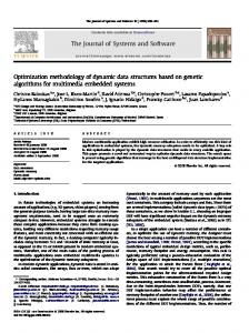
The solution, to this and a growing number of related problems, turned out to be the Voronoi diagram, which is a tiling of the plane that assigns each possible map location to its nearest data object. The result, for point data, is a set of convex polygons ("bubbles"), each with a data point as its nucleus (Figure 2). The common boundaries between bubbles indicate when they are adjacent, and this set of adjacencies forms the Delaunay triangulation, which is frequently seen in TIN terrain models. From its very definition, this triangulation is unique for any particular data set. In addition to providing a consistent definition of adjacency for unconnected objects, the triangulation can also be used to specify a spatial partial-ordering with respect to some view-point location (Gold, 1987). Since the triangulation is the network of all adjacency relationships, where adjacenc means that two "bubbles" have a common boundary, the Delaunay trP angulation is the spatial data structure for the Voronoi spatial model. Each map object has an associated bubble, or tile, and the collection of these bubbles tile the map area completely. The "nearest" definition for assigning any location on the map to a specific map object or tile is not restricted to point data: it is completely general. Subsequent work has concentrated on the Voronor diagrams of points lus line segments. To achieve this, however, the concept of “nav 'i gating" a map must be reviewed.
If, at all times, the spatial adjacency structure of the map is to be retained, then it should be possible to take a data point and steer it through the network -- without breaking the network of triangles that express the spatial relationshi s of the tiles or bubbles making up the map. (The utility of th Ps process will be seen shortly.) If one visualizes the situation as a set of contiguous bubbles, then it is easy to imagine that one of them could be moved as a local process while disarranging Only its immediate neighbours. (It is this property that guarantees the purely local update of the Delaunay triangulation.) The details of this process have been described elsewhere (Gold, 1990b). Once a point may be moved through space using purely local a few simple modifications permit more complex processes, operations. For example, the creation of a new data point may be achieved by: A) a simple search to find a nearby existing point: B) splitting this one bubble into two, creating a new bubble and data
251
point by "cellular fission"; and C) moving this new point (and its bubble) to its final destination. Deletion of the point follows the
same scheme in reverse, in all cases preserving the spatial data
structure (the Delaunay triangulation).
The creation of line segments follows directly. Since a line is the
focus of a moving point, the previous split/move process may, if desired, be used to create a trailing line segment that preserves all the adjacency relationships of the point during its travels. Figure 3 shows the Voronoi regions formed around a set of points, followed by the result of generating a line segment as just described. Further details are found in Gold (1990b).
All of these operations are local, and rapid. Visualizing the moving point as the cursor of a digitizer, line segments and points may be constructed as they are defined and inserted directly into the data structure. Since the moving point is functionally equivalent to a pen or cursor, including pen up/down equivalents, usage is almost intuitive. The result of the foregoing spatial model is a "bubble map", with each point or line segment being the nudleus of a tile or bubble. These tiles are convex for point sets, but include parabolic boundaries between adjacent points and lines for sets of points plus line segments. Potential applications for these bubbles include "area-stealing" interpolation (Gold 1989) and polygon skeleton generation (Gold 1990b) for centroid or labelling applications, as well as missing census district type interpolation (e.g. Gold 1990a). At any moment in time the "pen" has its own bubble, and hence its own set of neighbours. Examination of this neighbour set permits
ready navigation of the "obstacles" already in its path, including prevrous parts of the current line segment. Thus too-close approach to a neighbouring object may, depending upon the application or situation, trigger an intersection operation, a snapping-to operation or a rejection operation whereby a collision-avoidance mechanism prevents pen coordinates from intersecting an existing object. This forms the basis of 'Navigator", an attempt at an intelligent digitizer, that is presently under development. This is intended to be a proof-of-concept of the Voronoi or "bubble" spatial model. It is hoped that subsequent projects will follow. The "invasive" navigation process ust described serves to update the data structure with a moving po nt. A "non-invasive" query also exists that steps through the data structure, maintaining the "current closest object" to the cursor -- which is merely the tile within which the cursor falls. This automatic flagging of the closest object permits easy connection of polygon boundary segments. As line segments have two sides, the tile for a line segment has two parts, one for each side. Thus polygons are defined as the sum of the relevant tiles (Figure 4), and are not explicitly stored as data records. They may, however, be labelled by pointing at any appropriate tile within a boundary composed of points and
252
line segments, and labelling the other interior tiles by a triangulation-based form of flood-fill algorithm. It is also worth noting that the non-invasive query is equivalent to the point-inpolygon problem, thus providing an elegant local solution to this problem rather than the line-intersection method previously described. APPLICATIONS OF A DYNAMIC SPATIAL DATA STRUCTURE In the previous digitizing application, immediate query would permit immediate updating of data entry errors -- whether unwanted line crossings, dangles, gaps, unclosed polygons, etc. This would certainly s eed up the normal digitizing process, as the human preference Ps to complete a portion of a map while one is thinking about, and understands, it. Temporal skipping (waiting for the rebuild operation) is even worse than spatial skipping (looking back and forth between map, screen,keyboard, etc.) Immediate query could be used in a variety of other GIS applications, where its absence is a continual irritant. Any time that a sequence of changes are desired, with the next change depending on examining the previous one, waiting until "tomorrow" is at the least annoying, and frequently worse. Examples include landscape modelling, where it is desirable to try one layout of the grounds, examine it, make small changes, and repeat the process. It is hard to remember what one was thinking about yesterday when a chan e was made, and even worse to remember choices made before that s Any type of "what-if" nodelling that depends on significant user interaction is therefore all but precluded by non-dynamic SDS's, A particular example is forest management, where the economic consequences of a forest cutting decision need to be evaluated and adjusted in an iterative fashion in order to achieve both economic and environmental objectives. Time based CIS may sometimes be considered to consist of the sequential insertion and deletion of map objects (e.g. polygons and boundaries), as in the frames of a movie. This is not viable without a dynamic SDS. Area-stealing interpolation involves the insertion and deletion of the sampling point (Gold, 1989). Again, only dynamic maintenance makes this feasible. In the case of statistical estimates the data points themselves need to be deleted and re-inserted (Gold, 1990a). Any type of flow modelling, where individual particle movement depends on the action of its neighbours, is all but prohibitive without dynamic SDS's. Finite difference methods may be possible, because the attribute data base may be updated dynamically, as the polygons themselves need not move. This, however, only emphasizes the handicap of using a spatial data structure without dynamic update. If it is available for attribute data, it should exist for spatial data!
253
CONCLUSIONS I have reviewed the basics of dynamic data structures, both traditional and spatial, and examined the reasons why dynamism is not always easy to achieve. The importance of the underlying spatial assumptions has been emphasized, and a new spatial model -the Voronoi -- proposed. Recently gained experience, e.g. at the previous EGIS conference and in a new position in a research chair in forestry and geomatics, suggests that major concerns of operational GIS usage centre partly on rapid "what-if" queries after data modification, and even more on the ability to update a nap and validate that update in the same session, thus dramatically reducing the time taken to complete data input or updating. While not necessarily the appropriate approach when raw data is received in a batch form, e.g. from scanning, a large number of GIS operations would greatly benefit from the existence of a truly dynamic spatial data structure. It is hoped that the proposed Voronoi spatial model, being the basis for one fully dynamic spatial data structure, will be found useful in a variety of applications. ACKNOWLEDGEMENTS The funding for this research was made possible by the foundation of an Industrial Research Chair in Geomatics, jointly funded by NSERC and the Association de l'Industrie Forestière du Québec. REFERENCES Gold, C.M. (1990a), Neighbours, adjacency and theft -- the Voronoi process for spatial analysis. Proceedings, EGIS '90, Amsterdam, April 1990, pp. 382-391. Gold, C.H. (1990b), Space revisited -- back to the basics. Proceedings, Fourth International Symposium on Spatial Data Handling, Zurich, July 1990, pp. 175-189, Gold, C.M. (1989), Chapter 3 - Surface interpolation, spatial adjacency and G.I.S. IN J. Raper (ed.), Three Dimensional Applications in Geographic Information Systems, Taylor and Francis, Ltd., London, pp. 21-35. Gold, C.H. (1987), ordering of Voronoi network6 and their use in terrain data base management. Proceedings, AUTO-CART0 8, Baltimore, March 1987, pp. 185-194. Herring, J.R. (1987), TIGRIS: Topologically Integrated Geographic Inforration System. Proceedings, AUTO-CART0 8, Baltimore, March 1987, pp. 282-291.
Figure 2. The Voronoi regions of a simple point data set, showing the Delaunay triangulation.
Figure 1. Part of a B+ tree, showing the pointer structure.
\
Figure 3. The point set of Fig. 2 with a line segment developed as point 18 was split from point 17 and moved away
I
.s
I
Figure 4. A simple polygon and associated Voronoi regions: points P and Q are inside, R and S outside. Also shown is a buffer zone around the polygon boundary. 255