or with entcsmacro.sty for your meeting. Both can be found at the ENTCS Macro Home Page.
Visualization of Spatial Data Structures on Different Levels of Abstraction Jussi Nikander1 ,5 Ari korhonen
2 ,5
Department of Computer Science and Engineering Helsinki University of Technology Espoo, Finland
Eiri Valanto
3
Kirsi Virrantaus
4
Department of Surveying Helsinki University of Technology Espoo, Finland
Abstract Spatial data structures are used to manipulate location data. The visualization of such structures faces many challenges that are not relevant in the visualization of one-dimensional data. The visualized data can be represented using several different types of visual metaphors. These metaphors can be divided into several different levels of abstraction depending on the purpose of the visualization. This paper proposes a division of data structure visualization into four levels of abstraction, and shows how these abstractions can be taken into account in the visualization of spatial data structures. Keywords: Visualization, spatial data algorithms, abstraction,
1
Introduction
Spatial data structures are structures that store spatial data. Spatial is a term, which is used to refer to located data, for objects positioned in any space [5]. Spatial data is used in many areas of computer science, like Geographic Information Systems (GIS), robotics, computer graphics, and virtual reality. Algorithms that manipulate spatial structures are called Spatial Data Algorithms (SDA). Spatial Data Structures are based on regular non-spatial data structures like arrays, lists and tree structures, as well as the algorithms that manipulate these 1 2 3 4 5
Email:
[email protected] Email:
[email protected] Email:
[email protected] Email:
[email protected] This work was supported by the Academy of Finland under grant number 210947 c 2006
Published by Elsevier Science B. V.
Nikander et al
fundamental structures. However, much of the complexity of spatial data structures comes from the multidimensionality of the data. Two- and three dimensional variations of efficient algorithms make algorithm development more challenging. In the GIS literature there is a core set of fundamental as well as advanced spatial algorithms and data structures. However, no comprehensive textbook exists on the topic. Spatial data and algorithms for manipulating located data are an integral part of geoinformatics, a branch of science where information technology is applied to cartography and geosciences. Geoinformatics is closely related to cartography, and therefore illustrations, such as maps and other diagrams, are often used. For people in this field of study, graphics are a familiar and natural way of illustrating the work. Software visualization (SV) is a branch of software engineering that aims to use graphics and animation to illustrate the different aspects of software [10]. It is typically divided into two subdivisions: program visualization and algorithm visualization [8]. In both subdivisions it is important to be able to differentiate between the various levels of abstraction in the visualization. For example, a linked list implemented using two arrays can be visualized by showing the arrays and their contents. Such a visualization shows the implementation-level details of the list, but makes it hard to grasp its logical structure, which can easily be seen when the list is visualized as nodes connected by references. In this paper we will concentrate on the algorithm visualization (AV) side of SV. One of the main uses for SV is in pedagogy, and numerous SV systems have been developed for teaching. For examples, see [3,6,9]. In pedagogy, however, visualization does not have any intrinsic value. As noted by Hundhausen [4], the learners must be actively involved in activities where algorithm visualization is used in order to get better learning results. The graphic nature of spatial data algorithms and its applications makes SV a natural tool for teaching them. The data handled by spatial algorithms is multidimensional, and therefore the natural visualization for input, output and the solution process is a map or a diagram. Without using graphics, it is much harder to explain spatial algorithms or data structures. Thus, we are currently extending the TRAKLA2 visualization system [6] to include SDA. We are focusing on the structures and algorithms required in geoinformatics, a branch of science where information technology is applied to cartography and geosciences. We are unaware of any other work that applies SV techniques to spatial data structures. In this paper, we will propose a division of algorithm visualization into different levels of abstraction and describe how these levels can be mapped into the visualization of data structures in general. We will extend the category fidelity and completeness from the taxonomy of Price et al [8] in order to give a better insight into the various needs of pedagogical systems that “take liberties to provide simpler, easier-to-understand visual explanations”. The idea is to name four different levels of “visual metaphors that present the behavior of the underlying virtual machine”. We will apply these levels of abstraction in the visualization of SDA aimed at teaching the topic to students of geoinformatics. The rest of the paper is organized as follows. In Section 2, we introduce our 2
Nikander et al
model of different levels of abstraction in visualizing data structures. In Section 3, we discuss how this model can be applied to the visualization of spatial data structures. Finally, Section 4 discusses how the different levels of visualizations can be used in teaching SDA. concludes the paper.
2
Model for Data Structure Abstractions
A data structure (DS) can be defined as a collection of variables, possibly of several different data types, connected in various ways. An abstract data type (ADT) is a set of (abstract) items with a collection of operations defined on them. Separate definitions for the logical (ADT) world and for the physical (DS) world are essential for many reasons. First, these distinguish the design from the implementation. The definition of an ADT does not specify how the data type is implemented and implementation level details are hidden from the end user of the ADT. This hiding of the implementation details is known as encapsulation. Second, the concept of an ADT is an important principle used for managing complexity through abstraction. The irrelevant implementation details can be ignored in a safe way. This is also the way humans deal with complexity. We use metaphors to assign a label to an assembly of concepts and then manipulate the label in place of the assembly. Third, reusability is one of the key principles in software engineering that can be promoted by designing general purpose data structures suitable for many tasks, i.e., by implementing data types suited for several algorithms. In software visualization, we are interested in illustrating the organization of the related data items whether they are abstract or not. The same data items can be represented in several levels of abstraction depending on the purpose of the visualization. However, this need for granularity is not only biased to these two extremes (DS and ADT). For example, a binary heap is a priority queue ADT that is implemented as an array. Between these two levels of abstractions, it has a well known representation in which a binary heap can be visualized as a binary tree. In the following, we will fine tune the concept of data type abstractions in order to create a model that gives a deeper insight into the world of data structure implementations and the conventional visual notations used in text books. We will claim that only a small number of basic structures are required in order to implement any data structure. Furthermore, basic structures all have widely-accepted visualizations, or canonical views. These views can, in turn, be used to illustrate any data structure defined using these basic structures. 2.1
Simple example
Let us start with an example illustrated in Figure 1(a), which shows data structures visualized on four different levels of abstraction. There are two example structures shown on the figure, a binary heap on the left and a red-black-tree on the right. We will first focus on the visualization of the binary heap. A binary heap is typically implemented using an array. The canonical view of an array is shown on the lowest level in the figure. An array can be used to implement a binary heap by imposing a set of semantics to it: the child nodes of the node i are in positions 2i and 2i+1, and for each node the heap property “the parent is smaller 3
Nikander et al Red−black −tree
Binary Heap
Queue
DB
Level of abstraction
Applications 2
Representations 7
Array
B K
4
List
5 8
9
A
C H
M
B
Data Structures
K
A 2 4 5 7 8 9
H
M
C
Basic Structures
Tree
(a) Levels of abstraction in data structure visualization
Graph
(b) Canonical views of the basic structures
Fig. 1. Different visualizations
than or equal to the children” holds. An instance of a binary heap is shown on the second-lowest level in Figure 1(a) (data structure view). On this level, the heap is visualized as an array, and therefore the visualization accurately reflects how the data structure is implemented. However, in the array visualization, it is quite hard to see whether the heap property holds. The heap property is easier to see when the data structure is shown using the binary tree representation (representation view). Finally, a binary heap can be utilized, for example, in a network router simulation (application view). Different packets can have different priorities, and the priority queue could be abstracted into a black box where the internal structure is not shown at all. The packets go in from the right, and forwarded packets come out from the left. If packets are dropped, they are shown below the visualization. 2.2
Basic structure level
In general, a basic structure is a generic data type (a skeleton) that is used to implement a particular data structure. For example, arrays, linked lists, trees, and graphs are basic structures. These are archetypes, reusable basic building blocks for creating structures, and all the data structures used in text books can be implemented in terms of these archetypes. For example, an adjacency list is a composition of an array and a number of linked lists. The canonical views of the basic structures are commonly accepted and used, for example, in most text books. They are simple and easily recognized visualizations, which anyone familiar with data structures will immediately identify as a certain type of structure. Examples of the canonical views can be seen in Figure 1(b). The canonical view of an array is a set of boxes arranged side-by-side, with each box holding a single data item. Similarly, the canonical view of a list is a group of nodes arranged in a line, where each node has a reference (line with possibly an arrow at the end) to its successor. The first node of the list is the leftmost one. The canonical view of a (rooted) tree is a number of nodes arranged to levels in a topdown-fashion, where each node has a reference to its children, and all nodes that are from a given distance from the root node are on the same level. The canonical view of a graph is a group of nodes, each of which has references drawn to its successors, 4
Nikander et al
typically arranged using a visually pleasing and intelligible layout. From the visualization point of view, Basic Structure Level is the lowest level of abstraction that we are interested in presenting. This level contains the canonical views that can be used to visualize any data structure defined using the basic structures. Still, even these canonical views are abstractions. For example, an array is a commonly used term in computer science to denote a contiguous block of memory locations, where each memory location stores one fixed length, and fixed-type variable. However, an array can also refer to a structure composed of a (homogeneous) collection of variables, each variable identified by a particular index number. Most programming languages do not directly support this latter form of definition due to its abstract nature. Thus, there are possibly several different implementations for arrays. However, the low-level abstraction behind each of them is common for all of the implementations, and can be represented in a uniform way 6 . As we can see, basic structures do not have semantics. The definition of what is an array does not dictate the data types nor the order of the items within. The design and analysis of algorithms, however, require an organization of information in such a way that the computing can be performed efficiently. Similarly, we need to illustrate the actual data and other restrictions in order to come up with a meaningful illustration. The fundamental idea behind basic structures is to reuse them many times to represent several data structures all having different semantics. For example, an array can be the basic building block for both hash table and binary heap. Similarly, in visualization of these basic building blocks we can have a single reusable representation for all data structures that utilize arrays. This makes it possible to visualize any data structure with a handful of different representations. 2.3
Data Structure Level
At Data Structure Level we have data structures that are implementations for conceptual models that encapsulate particular ADTs. This conceptual model defines the basic structures used to implement the model, as well as the type constraints that lay the foundation for the implementation. The corresponding data structure is an implementation that defines also the operations needed to change the structure. For example, a red-black-tree is a data structure that has the basic structure of binary tree, and implements an ADT called dictionary (operations search, insert, and delete). An example tree is illustrated in Figure 1(a) (red nodes are shown with double circles). On Data Structure Level, the data structures are visualized using the canonical views defined in terms of the basic structures. Therefore the visualizations accurately reflect the actual implementation of the data structure, and show all (relevant) parts of the structure. In the visualization, we are most interested in the layout and the question whether it satisfies the constraints of the data structure. The concept of rotation in red-black trees, for example, can be expressed in terms of changes in this layout (i.e., moving nodes and arcs between nodes). Of course, the actual code can be illustrated as well, for example, as a pseudo-code. 6
Of course, there are several ways to illustrate arrays, but the canonical visual notations commonly used are all equal in such a way that a person can easily grasp the idea of an array from each of them.
5
Nikander et al
On the data structure level the layout of the visualization can be modified in order to give the viewer a visual hint of what kind of data structure is visualized, or to show some additional information about the different parts of the structure. For example, the nodes of a red-black tree are typically drawn either red or black. 2.4
Representation Level
A single data structure can often be represented in several ways. In our definition, the Representation Level contains visualizations that do not neccessarily reflect the actual implementation, but still show all the data stored in the structure. For example, a binary heap can be represented as an array, which reflects its actual implementation, or as a binary tree that better illustrates the logical structure of the heap. Therefore, different representations form a level of abstraction where the visualizations can be modified to hide the “physical” characteristics of the data structure in order to make some implicit characteristics explicit. We call these abstractions Representation level visualizations. On representation level, the visual methaphor used to illustrate the data structure can be changed in order to bring out the desired characteristic of the structure more clearly. For example, a red-black tree can be used to implement a B-tree [2], and therefore it can be visualized as such as well. In Figure 1(a), a 2-3-tree representation is used for the red-black tree in Representation Level. Furthermore, on the Representation Level, some visualizations no longer conform to any of the canonical views illustrated in Figure 1(b). It should be noted, however, that any data structure can be visualized using canonical views. Sometimes, however, customized visualizations are better for grasping some important aspects of the structure. Alternate visualizations are especially useful when the data stored in the structure is multidimensional. In the canonical views, there is only one dimension that can be used for showing the relationships between the data elements: the visualization of the data key values. If the elements are, for example, points in two dimensionsional space, it is hard for the viewer to grasp the relationships among the elements in one-dimensional visualization. If the points are drawn into twodimensional plane, however, it is more convenient to see the relationships (e.g., distance, direction) among different data points. 2.5
Application Level
The top level of abstraction is called Application Level. Visual metaphors, where the information in the data structure is not fully visible, are considered to be on this level. This is called application level since almost all applications that use graphics to illustrate the data show only relevant data items instead of the whole dataset. Typically only those applications that are used for software visualization can show all the data. Typically, on this level, we illustrate the data in domain specific ways that omit most or all of the data structure’s details. For example, B-trees are often used as database indexes or storage structures as illustrated by the database symbol in Figure 1(a). This view hides all the details of the implementation Therefore, on the Application Level, the data structure visualization is analogous to the definition of 6
Nikander et al
an ADT. The interface is defined, but implementation is hidden. 2.6
Combined Levels
Software visualization techniques and tools can be utilized in many other disciplines as well. Especially, there exist abstractions that have proved to be particularly important for many disciplines. The idea behind the categorization of these abstractions is that we can utilize the same components and concepts over and over again and take advantage of the prior work done. In addition, when visualization is used to illustrate a concept or a data structure, it is often useful to have several visualizations that use different views on the same data structure simultaneously. For example, by showing how a binary heap evolves while new elements are added or removed in both array and binary tree visualization simultaneously can help the viewer to see how the logical and physical structure of the heap relate to each other. Some application areas are intrinsically visual. For example, in GIS applications, the typical representation is a map. However, the underlying data structures and their visual counterparts are basically the same as, for example, in software visualization. Thus, we need to make a distinction between the application level visualization and the illustrations for the underlying data structures and algorithms. However, no matter what kind of application we have in mind, it can be reduced to those basic building blocks through the levels of abstraction, as we will see in the next section.
3
Visualization of Spatial Data Algorithms
Spatial data algorithms process data which is naturally visualized as maps. In this section, we show how the model from previous section is applied to SDA. Specifically, we present a common geoinformatics problem, called map overlay, as an example and describe how it can be visualized using several visualizations on different abstraction levels. On the application level, we typically illustrate the data in some form. In GIS applications both source and result data sets can be visualized as maps of some type. Thus, application level visualizations can give good overview of the problem, particularly as specialists in geoscience and cartographic fields are used to handle and understand maps. However, while visualizations in GIS applications give a good illustration of the data, they omit all details of the data structures used. The problem of combining two different maps to produce a new map with information from both maps’ domain is called map overlay. The interest often lies in discovering areas where some properties coincide. For example squirrel habitat areas could be combined to a vegetation layer to get a map presenting areas where squirrels are found in coniferous forests. The description of map overlay as a combination of two map layers belongs to the highest abstraction level in our conceptual framework (Figure 1(a)). We have two maps presenting four urban municipalities in Helsinki metropolitan area and postal code areas in the same region, respectively. Our problem is to find 7
Nikander et al
which municipality each postal code area belongs to and to locate areas where postal code areas cross municipality boundaries. Map overlay can provide a solution to these questions. Figure 2(a) illustrates the source maps as well as the resulting overlay. In order to solve a problem with a computer, the problem has to be represented formally in some way. Typically, mathematical presentations are used to store map data. Such presentation also gives a view of the data that is independent of any computerized data structure implementation. Even if a mathematical presentation hides all the physical details of the data structure, it clearly shows logical connections between data elements, and therefore belongs to the representation level. In geoinformatics, examples of mathematical presentations are Voronoi diagrams and their dual, the Triangular Irregular Network (TIN) [7]. In GIS, data can be represented using two models: either vector or raster model. In vector representation, data is presented as points, lines or polygon objects, which have spatial location data associated to them. Polygons can be used to construct polygon maps, lines can be used in graphs, and point sets can be structured into TIN-models or Voronoi-diagrams. The advantage of TINs and Voronoi diagrams is that discrete measured points make a structure that supports, for example, interpolation and visualization. A raster model utilizes a regular grid that divides the represented area into equal sized cells. Each cell contains an associated value that represents the values of the respective area. The map overlay problem can be solved by applying the vector or raster model. In our example, we use map overlay operation in vector format. In the vector format, the areas to be overlayed are typically represented as polygons. Polygon is an abstraction of a group of points and the references connecting them, and a polygon map visualization of the data belongs to the Representation Level. Thus, we have two polygon maps which are overlayed by intersecting the polygon boundaries. The map overlay first uses some method, for example the line-sweep algorithm, to locate intersecting lines. The intersection points are then used to create new polygons, which form the resulting map. Figure 2(a) iv shows a detail on Helsinki boundary where the map overlay divides a postal code are into two polygons. The rectangle in Figure 2(a) iii highlights the location of the detail. To achieve an efficient solution on a computer, a suitable data structure is needed for storing the mathematical model. Typically, there are several possible data structures that can be used to store each model. The model itself defines an abstract data type of sorts: it tells how the data can be manipulated and how it is structured, but does not define how the data structure is to be implemented. The data structure used to implement a mathematical model therefore has a well-established set of semantics and thus is a conceptual model that encapsulates a particular ADT. For map overlay, one possible data structure is Doubly Connected Edge List (DCEL) [1]. The DCEL consists of vertices, polygon faces and half-edges that connect vertices. Each vertex has a location and connection to a edge that originates at the vertex. Every polygon face has information of a half-edge on its outer boundary and a list containing each hole in the face. Each edge is divided to two half-edges. A half-edge has information of its origin vertex and twin. Destination is not needed because it is the same vertex as twin’s origin. In addition, a next and a previous 8
Nikander et al
i
ii
iii
iv
(a) Map overlay problem i) postal code areas, ii) munic- (b) DCEL structure presentation of municipality boundary source maps iii) map overlay result, iv) ipality boundaries detail where municipality boundary divides a postal code area into two polygons Fig. 2. DCEL visualizations
half-edge is connected to each half-edge as well as the incident polygon face. Figure 2(b) shows the simplified municipality boundaries as DCELs. On the left is a visualization of a (partial)structure shown as a graph and on the right as a group of arrays. For a DCEL structure a graph visualization can be considered a Representation Level visualization, since it hides a lot of the relations between the data items. For example, each half-edge knows its successor and predecessor edges, but these edges are typically not explicitly shown in a graph visualization. Since a DCEL structure contains spatial data, the best graph visualization for showing its logical structure takes the coordinates of the data items into account. Therefore, the different points and half-edges are drawn in their correct coordinates. Using DCEL map overlay is solved by first combining both map layer’s DCEL structures into an invalid DCEL. This is then examined and modified to form a valid structure. Finally, the basic structures used for the implemntation of DCEL are visualized on the right in Figure 2(b). A DCEL contains three types objects: vertices, faces and half-edges. Therefore, DCEL implementation requires at least three structures for storing the data. A natural way to build a DCEL is by using three arrays containing the corresponding information. On the Data Structure Level, basic canonical representations used to visualize spatial data structures are identical to canonical views of any other data structure.
4
Discussion
In this paper, we have described how data structure visualizations can be divided into four distinct levels of abstraction, how these levels differ from each other, and how they can be applied to visualization of different kinds of data structures. Especially, we have shown how visualization on different levels can be applied to spatial data structures and algorithms. Our example, map overlay, was from the field of geoinformatics which, as a discipline, is very visual in nature. Most geoinformatics problems involve graphical views in the description, solution, and the solution process. For the people in the field, visualizations are a natural and extremely common way for processing and representing data. Therefore visualizations are also a very good tool for teaching 9
Nikander et al
aspects of geoinformatics, including SDA. Since spatial data structures contain two-dimensional data, traditional algorithm visualization techniques can be sub-par. Traditionally, the focus of the visualization has been to show the composition of the data structures. A graph visualization, for example, shows the vertices and edges in a visually appealing fashion, and a tree visualization is optimized to show the relations between tree nodes. When the data stored in the structure is one-dimensional (like numbers or strings), this also shows the relation between the data elements. When the data is two-dimensional, however, the relations between different parts of the structure do not typically give a comprehensive view of the relations between data items. DCEL, for example, is typically used to represent vector maps in geoinformatics. Depending on the level of abstraction used and the type of visualization selected, the information one can gain from a DCEL varies a lot. When viewed as arrays, the visualization is good for understanding the minute details of the implementation, but does not give a very good overview of the data it represents. If viewed as a graph such as in Figure 2(b), the visualization gives a good view of the data being represented, but omits many of the implementation-level details. In order to effectively visualize some SDAs, we clearly need several visualizations simultaneously. One visualization to show the inner composition of the data structure in question, and another to give an easily understood view of the data being represented. This effectively expands the multiple views category of [8], which measures the degree of multiple synchronized views the visualization can provide. The taxonomy discusses views of different granularity. We, on the other hand, require views that use different graphical metaphors to show the data and thus make different aspects of the logical structure explicit.
References [1] de Berg, M., M. V. Kreveld, M. Overmars and O. Schwarzkopf, “Computational Geometry: Algorithms and Applications,” Springer, 2000 pp. 29–33. [2] Guibas, L. J. and R. Sedgewick, A dichromatic framework for balanced trees, in: Proceedings of the 19th Annual Symposium on Foundations of Computer Science, IEEE Computer Society, 1978, pp. 8–21. [3] Hundhausen, C. and S. A. Douglas, SALSA and ALVIS: A language and system for constructing and presenting low fidelity algorithm visualizations, in: Visual Languages, 2000, pp. 67–68. URL http://citeseer.ist.psu.edu/hundhausen00salsa.html [4] Hundhausen, C. D., S. A. Douglas and J. T. Stasko, A meta-study of algorithm visualization effectiveness, Journal of Visual Languages & Computing 13 (2002), pp. 259–290. [5] Laurini, R. and D. Thompson, “Fundamentals of spatial information systems,” Academic Press, 1992. [6] Malmi, L., V. Karavirta, A. Korhonen, J. Nikander, O. Sepp¨ al¨ a and P. Silvasti, Visual algorithm simulation exercise system with automatic assessment: TRAKLA2, Informatics in Education 3 (2004), pp. 267 – 288. [7] Okabe, A., B. Boots, K. Sugihara and S. N. Chiu, “Spatial Tessellations: Concepts and Applications of Voronoi Diagrams,” John Wiley & Sons, 2000. [8] Price, B. A., R. M. Baecker and I. S. Small, A principled taxonomy of software visualization, Journal of Visual Languages and Computing 4 (1993), pp. 211–266. [9] R¨ oßling, G., M. Sch¨ uler and B. Freisleben, The ANIMAL algorithm animation tool, in: Proceedings of the 5th Annual SIGCSE/SIGCUE Conference on Innovation and Technology in Computer Science Education, ITiCSE’00 (2000), pp. 37–40. [10] Stasko, J. T., J. B. Domingue, M. H. Brown and B. A. Price, “Software Visualization: Programming as a Multimedia Experience,” MIT Press, Cambridge, MA, 1998.
10