BIOLOGICAL SYSTEMS. Peter Drábik, Andrea Maggiolo-Schettini ...... CoRR, abs/0801.1687, 2008. [2] Federica Ciocchetta and Jane Hillston. Bio-pepa: A ...
DYNAMIC SYNC-PROGRAMS FOR MODULAR VERIFICATION OF BIOLOGICAL SYSTEMS Peter Dr´abik, Andrea Maggiolo-Schettini and Paolo Milazzo Dipartimento di Informatica, Universit`a di Pisa Largo B. Pontecorvo 3, 56127 Pisa, Italy Email: {drabik,maggiolo,milazzo}@di.unipi.it
Abstract We propose dynamic sync-programs, a bio-inspired automata-based formalism for the description and the modular verification of properties of biological systems. The formalism allows entities to be created dynamically, in particular by other already running entities, as it often happens in biological systems. Moreover, multiple copies of the same entities can be present at the same time in a system. Modular verification allows properties expressed as DACTL formulae (dynamic version of the universal fragment of CTL) to be verified on a portion of the model, rather than on the whole model. We show, as an example, the application of our approach to a biological case study, namely the EGF signalling pathway.
1. Introduction Model checking permits the verification of properties of a system (expressed as logical formulae) by exploring all the possible behaviours of the system. Recently, it has been successfully applied to analysis of biological systems (see e.g. [7, 5, 2]). However, model checking techniques have traditionally suffered from the state explosion problem. A method for trying to avoid such a problem is to use the natural decomposition of the system. The goal is to verify properties of individual components and infer that these hold in the complete system. A technique proposed by Attie [1] exploits the preservation of properties expressed with ACTL (the universal fragment of the CTL temporal logic) from components to whole systems in order to verify concurrent programs and synthesise systems from specifications. Attie uses a formalism called synchronisation skeletons [3] suitable for describing distributed systems. In [4] we proposed an extension of Attie’s approach for the description and the modular verification of biological systems. In particular, we defined sync-programs, an automata-based formalism of interactive systems which extends the formalism used by Attie by allowing processes to perform transitions simultaneously. Here we further extend the approach by allowing sync-automata (the components of a sync-program) to be created dynamically by other already running sync-automata. Moreover, we allow several instances of the same sync-automata to be
2
Dr´abik, Maggiolo-Schettini and Milazzo
executed concurrently, without any bound of the number of concurrent instances of the same sync-automaton. As our previous extension of Attie’s approach, also this further extension is biologically motivated. Indeed, in biological systems it is often the case that entities involved in the processes of interest (e.g. proteins) are synthesised by other active entities (e.g. the DNA). Moreover, it is very common that a number of copies of the same entities (e.g. proteins) are active at the same time. In what follows we give a formal definition of the syntax of dynamic sync-programs and their translation into Petri nets. The existence of such a translation implies that the formalism is not Turing-complete and that verification of the properties of interest is decidable. In order to shorten the presentation, we define the semantics of dynamic sync-programs by exploiting the translation into Petri nets and their semantics. Subsequently, we develop the modular verification approach for dynamic sync-programs by defining projection operations on their syntax and on their semantics, and by giving some results on the preservation of properties from components to whole systems. Finally, we apply our approach to a biological case study, namely the EGF signalling pathway.
2. Dynamic sync-programs 2.1. Syntax To model biological systems, we use a component-based approach. Each component represents a biological entity, e.g. a protein or an enzyme. The system will be modelled by a program consisting of a parallel composition of automata of different types. We assume a finite set of component types CT . For the purpose of developing a modular approach, the interactions between component types are indicated explicitly. We say that (not necessarily distinct) types i and j from CT interact directly, when one can perform an activity conditioned on the activity of the other and vice versa or when component of one type causes creation of a component of the other type. Direct interaction is distinguished from indirect interaction, which is mediated by a third party. We define an undirected interaction graph I (see e.g. Figure 1), where the nodes are types from CT and there is an edge between nodes i and j iff types i and j interact directly. Note that there can be loops in the graph, representing interaction of two components of the same type. We use notation iIj if there is an edge between i and j in graph I. By |I| we denote the set of nodes in I and by I(i) the set {j ∈ |I| | iIj}. By J ⊆ I we denote a connected subgraph J of I. In our approach, states of the components will be encoded by using atomic propositions. With every component type i a set AP i of atomic propositions is associated. The sets of atomic propositions are pairwise disjoint for all the types, i.e. if i 6= j then AP i ∩ AP j = ∅. We assume a function type : AP → CT that for an atomic proposition from AP i gives its type i. Analogously, function types yields a multiset of types of a set of APs.
3
DYNAMIC SYNC-PROGRAMS FOR MODULAR VERIFICATION
An individual component of a component type from CT is modelled by a finite state machine called sync-automaton. Definition 1. A sync-automaton AIi , where i is a component type and I is an interaction graph, is a tuple (Si , Si0 , SCi, CCi , Ri ): • Si ⊆ P(AP i ) is the set of states • Si0 ⊆ Si is the set of initial states • SCi is a set of labels of the form ∧k∈L Uk :Vk where finite L ⊆ N and for every k ∈ L there is a j ∈ I(i) such that Uk , Vk are sets of atomic propositions drawn from AP j or their negations. A label from SCi is called a synchronisation condition • CCi is a set of labels of the form new(∧k′ ∈K Wk′ ) where finite K ⊆ N and for every k ′ ∈ K there is a j ∈ I(i) such that Wj is a set of atomic propositions drawn from AP j or their negations. A label from CCi is called a creation condition • Ri ⊆ Si × SCi × CCi × Si are the moves between states. Each state of a sync-automaton AIi is a truth value assignment to atomic propositions of component type i. Each move is labelled by a synchronisation condition sc and by a creation sc condition cc. We denote a move from state si to state ti with labels sc and cc by si − → ti . This cc
move intuitively means that automaton AIi can move from si to ti if there are concurrently performed moves of sync-automata of types in I(i) satisfying condition sc. By performing the move, automata described by cc are created. An example of a sync-automaton can be seen on Figure 2. The component type uses two atomic propositions, A and B. The two states of the automaton are {A, B} and {¬A, B} with the former chosen to be initial. Moves between states are labelled by synchronisation and creation conditions. Nucl M:¬M ∧ B:¬A new({X, ¬Y })
Lyso
Eff
¬A B
AB Egfr
Endo
Figure 1: The interaction graph of the model of the EGF pathway (dashed lines – creation).
NOSYNC
NOSYNC
Figure 2: Example of a sync-automaton and move conditions.
The synchronisation condition is a label in form ∧k∈L Uk :Vk and specifies requirements for automata of types from I(i) to synchronise with. For every k in L, the sets of propositions Uk and Vk are to be satisfied in the starting and ending state, respectively, of the concurrently performed move of a sync-automaton of a type type(Uk ) (see Figure 2). We remark that in the synchronisation condition of a move of a sync-automaton of type i there can be multiple references to the components of a type j, referring to different instances
4
Dr´abik, Maggiolo-Schettini and Milazzo
of sync-automata of such a type. References to other instances of the same type i are also allowed. Moreover, note that it is possible for L to be empty. Intuitively, this means that the sync-automaton AIi does not have any requirements on other sync-automata. We write NOSYNC a synchronisation condition of this form, i.e. ∧j∈∅ Uk :Vk , as NOSYNC . Move si −−−−−→ ti represents an autonomous move of AIi . The creation condition is a label in form new(∧k′ ∈K Wk′ ) that specifies sync-automata that are to be created. For every k ′ in K, the set of atomic propositions (or their negations) Wk′ encodes an initial state of sync-automaton AIj for j = type(Wk′ ) which will be created having this initial state. In case the multiset K is empty, the creation condition is not displayed. For an example see the move on Figure 2 from {A, B} to {¬A, B} which specifies a creation of an automaton with initial state {X, ¬Y }. By running in parallel sync-automata of types related by an interaction graph, we obtain a sync-program. Note that a sync-program can contain none or multiple sync-automata of any component type. Definition 2. Let I be an interaction graph. A sync-program is a tuple P I = (si1 || . . . ||sin ), where each si is an initial state of sync-automaton AIj of type j = type(si ) where j ∈ I. The creation conditions on the moves of all sync-automata are well formed, i.e. for every creation condition new(∧k′ ∈K Wk′ ), each Wk′ describes a unique state s′ of a sync-automaton of type in I and s′ is initial. 2.2. Sync-programs as Petri nets A dynamic sync-program can be represented as a Petri net. Intuitively, a place in the net represents a state of a component type, a transition embodies synchronisation of sync-automata and creation of new ones. Then number of tokens in a place represents the number of automata currently in that state. A Petri net consists of a Petri net graph and an initial marking. Note that the net graph is created from the set of all component types and is always finite. Then the initial marking is constructed according to the program. Definition 3. Given a set of sync-automata AI = {Ai | i ∈ |I|}, S we construct a Petri net graph GI = (SI , TI , WI ) as follows. The set of places is SI = i∈|I| Si . We assume a linear S k order on SI . The set of transitions TI is such that TI ⊆ SI∗ × SI∗ where SI∗ = ∞ k=1 SI , with k−1 1 k SI = SI and SI = SI × SI . Set TI contains transitions of the form tr = (In, Out) with In ordered. We denote with In i and Out i the i-th element of In and Out, respectively. Moreover, (In, Out) ∈ TI if and only if In and Out are minimal tuples and Create ⊆ N × P(AP ) is a minimal set satisfying: ∧k∈L Uk :Vk
1. for all i ∈ {1, . . . , |In|} there is a move In i −−−−−−−−−→ Out i in Atype(Ini ) such that new (∧k′ ∈K Wk′ )
• there is an injective mapping inst from L to {1, . . . , |In|} − {i} such that for all k ∈ L for all p ∈ Uk : In inst(k) (p) = tt and for all p ∈ Vk : Out inst(k) = tt
DYNAMIC SYNC-PROGRAMS FOR MODULAR VERIFICATION
5
• {(k ′ , Wk′ ) | k ′ ∈ K} ⊆ Create 2. for all i ∈ {1, . . . , |Create|}: Out |In|+i = ci where Create i = (ji , ci) The set of arcs WI ⊆ (SI × TI ) ∪ (TI × SI ), consists of the union of the following sets • {(s, |Move|, tr) | tr ∈ TI ∧ tr = (In, Out) ∧ Move = {j | (s, j) ∈ In} ∧ Move 6= ∅} • {(tr, |Move|, t) | tr ∈ TI ∧ tr = (In, Out) ∧ Move = {j | (t, j) ∈ Out} ∧ Move 6= ∅}. In the definition of the encoding of dynamic sync-programs into Petri net graphs we have represented a transition as a pair of tuples (In, Out). Tuple In consists of the starting states of the moves that synchronise in the step represented by the transition. The first |In| elements of tuple Out represent the ending states reached by such moves from the corresponding elements in In. The rest of tuple Out represents the initial states of the sync-automata dynamically created in this step. The set Create is used to collect such initial states from the creation conditions of the moves involved in the transition. Minimality of In, Out and Create ensures the indivisibility of the synchronisation, and guarantees that all the considered synchronising moves can be grouped in a single transition of the Petri net. With this encoding we have that Petri nets can be considered as an alternative representation for sync-programs. Petri nets are very intuitive and allow the modeller to have a comprehensive view of the system. However, since they are not compositional, they are not suitable neither for modular modelling, nor for modular verification. The existence of the translation of syncprograms into Petri nets is very important since it implies that the formalism is not Turingcomplete and that verification of the properties of interest is decidable. 2.3. Semantics Now we exploit the translation of dynamic sync-programs into Petri nets to give a formal semantics to such programs. The semantics could also be defined directly on the sync-programs (as in the non-dynamic case in [4]). However, we choose not to follow the latter approach here for reasons of space limitation. The semantics of a Petri nets is given in terms of a transition system. Since we consider only nets obtained from the encoding of sync-programs, we can give a slightly richer transition system that includes some information about the sync-automata involved in each transition. A marking of a Petri net graph is a multiset of its places, i.e. a mapping M : SI → N. We say that a marking assigns a number of tokens to each place. Note that markings can be added like any multiset: M + M ′ = {s → (M(s) + M ′ (s)) | s ∈ SI }. The execution of a Petri net graph GI = (SI , TI , WI ) can be defined as the transition relation →l on its markings, as follows: • for any t in TI : M →lt M ′ iff there is M ′′ : SI → N s.t. M = M ′′ + Σs∈SI WI (s, t) ∧ M ′ = M ′′ + Σs∈SI WI (t, s) and l = types(t)
6
Dr´abik, Maggiolo-Schettini and Milazzo • M →l M ′ iff there is t ∈ TI s.t. M →lt M ′
In words: firing a transition t in a marking M consumes WI (s, t) tokens from each of its input of its input places s, and produces WI (t, s) tokens in each of its output places s and label l contains types of automata that participate in the transition. These types are recorded for the purpose of compatibility of the semantics obtained through the translation in Petri nets and the direct semantics where they are necessary. We say that a marking M ′ is reachable from a marking M in one step if M →l M ′ for some l. We say that it is reachable from M if M →∗l M ′ , where →∗l is the transitive closure of →l , that is, if it is reachable in zero or more steps. A Petri net consists of a Petri net graph and of an initial marking M0 . The initial marking of a Petri net is obtained from the encoding of a sync-program. It contains as many tokens in a place representing an initial state of a sync-automaton from I, as there are instances of such initial state in program P I . For a Petri net NI = (SI , TI , WI , M0 ) the set of reachable markings is the set R(NI ) = {M ′ | M0 →∗l M ′ }. The reachability graph of NI is the transition relation →l restricted to R(N). Definition 4 (Semantics). The I-structure MI of a dynamic I-program P I is defined as the reachability graph of NI , where NI is the marked Petri net obtained by the encoding of P I . A transition (M, l, M ′ ) is in MI iff M →l M ′ is in R(NI ). A marking from MI is called an I-state. The set of initial sets of MI is a set of initial markings that is admissible by all automata types. A concept that will allow us to reason about properties of programs is that of path. A path in an I-structure MI is a sequence of I-states and transition labels π = (s1 , l1 , s2 , l2 , . . .) such that for all m, (sm , lm , sm+1 ) ∈ MI . A fullpath is a maximal path, and it is infinite unless for ′ ′ ′ ′ ′ ′ some sm there is no sm +1 and lm such that (sm , lm , sm +1 ) ∈ MI . Let π m denote the suffix of π starting in m-th I-state.
3. Subprograms and projections In order to develop our modular verification techniques we need two projection operations that allow us to restrict the syntax and the semantics of a sync-program to the components that have an influence on the satisfaction of a property of interest. A sync-subprogram represents the behaviour of a portion of a sync-program in isolation. We obtain a sync-subprogram by projecting a sync-program P I onto an interaction graph J ⊆ I. Graph J represents a subset (subgraph) of the set of all component types I. We denote the projection by the projection operator ↾J. In order to obtain P I ↾J we compute a J ′ ⊇ J which is a subgraph of I containing types of automata that can create (also by transitivity) automata of types in J. Then by projection P I |J ′ inspired by [4] we obtain the syntactical projection P I ↾J.
DYNAMIC SYNC-PROGRAMS FOR MODULAR VERIFICATION
7
Now, let J ′ be the graph that can be obtained through syntactical analysis of the component types as follows. The creation graph of J is a graph with vertices from CT . There is an oriented edge from i to j if there is a move in in AIi whose creation condition contains an initial state of automaton of type j. Subgraph J ′ is induced by vertices from J together with vertices from whose there is a path to vertices in J. Now denote X := J, Y := J ′ − J, Z := I − J ′ . The projection onto J ′ removes all automata from Z, namely those that neither are nor create (not even by transitivity) an automaton from J. This is defined as follows. Definition 5. Let J ′ ⊆ I be an interaction graph, where |J ′ | = {j1 , . . . , jk }. Let P I = (si1 || . . . ||sin ) with AIi = (Si , Si0 , SCi, CCi , Ri ) and si ∈ Si0 for each i ∈ |I|. Then P I |J ′ = (sj1 || . . . ||sjk ) with AJj = (Sj , Sj0 , SCj′ , CCj′ , Rj′ ) and sj ∈ Sj0 for each j ∈ |J| where: • SCj′ = {∧j ′ ∈L∩|J ′| Uj ′ :Vj ′ | ∧j ′ ∈L Uj ′ :Vj ′ ∈ SCj ′ }; • CCj′ = {new (∧j ′ ∈K∩|J ′| Wj ′ ) | new (∧j ′ ∈K Wj ′ ) ∈ CCj ′ }; ∧j ′ ∈L∩|J ′ | Uj ′ :Vj ′
∧j ′ ∈L Uj ′ :Vj ′
new (∧j ′ ∈K∩|J ′ | Wj ′ )
new (∧j ′ ∈K Wj ′ )
• Rj′ = {sj −−−−−−−−−−−→ tj | si −−−−−−−−−→ tj ∈ Rj }.
The projection contains only sync-automata from J ′ . Each sync-automaton has the same states as its counterpart in P I but the synchronisation and creation conditions on their moves concern only sync-automata from J ′ . We remark that a sync-subprogram P I |J ′ is still a sync-program ′ with interaction graph J ′ , hence it can be also denoted by P J . Thus, syntactical projection is defined as follows: P I ↾J = P I |J ′ where J ′ is obtained from the creation graph of J. To define the semantic projection, let us denote with s⌈J the projection of an I-state s onto a J ⊆ I. It is the greatest submultiset of s consisting only of states of sync-automata from J. A transition (s, l, t) in a I-structure can be projected onto J ⊆ I as follows: (s, l, t)⌈J = (s⌈J, l ∩ |J|, t⌈J). Projection of a I-structure MI onto J can now be defined as the transition relation consisting of the projections onto J of the transitions in MI . Note that it is possible that the transition label is an empty set, and the corresponding projected states can be both equal (synchronisation outside J was removed) or different (because of creation by an automaton outside J). However this does not cause problems, as for the purpose of verification the transitions of the former type are removed. Path projection π⌈J is obtained by projecting every transition of the path π onto J.
4. Modular verification In order to analyse the behaviour of a biological system we would like to verify properties of computations of sync-program P I representing the system. Assume, that property φJ only regards part of the system, in particular the part involving only components from J ⊆ I. We would like to check satisfaction of φJ on semantics of P I . In order to avoid the space explosion, we want to check it on a smaller and more abstract semantics, in particular semantics of P J = P I ↾J. By abstracting away some of the automata we lose some synchronisations,
8
Dr´abik, Maggiolo-Schettini and Milazzo
obtaining an overapproximation of the behaviour of P I . The essence of the verification can be expressed as equation Sem ◦ ⌈ ⊆ ↾ ◦ Sem, where Sem denotes the semantic function. In this section we assume that sync-programs contain no indirect synchronisations in the form of synchronisation conditions. If this is not the case, the program must be modified in a preprocessing step. We argue, that each computation being a fair path of the entire system projected onto J is present as a computation of P J . In the line of [4] we first prove the Transition projection and Path projection lemmas. By assuming fairness we avoid problems of losing the eventuality properties and we get the Fullpath projection lemma. Subsequently, we specify the logic suitable for describing the properties of dynamical syncprograms and finally we show the preservation of this logic. 4.1. Lemmas Lemma 4.1 (Transition projection). Let I be an interaction graph and MI the semantics of sync-program P I . For all I-states s, t in MI and all multisets l of elements from |I|, transition (s, l, t) is in MI iff for all J ⊆ I we have that (s, l, t)⌈J is in MJ , where MJ is the semantics of sync-program P J = P I ↾J. This lemma can be proved by using the definition of semantics and the definitions of both projections. The path projection result follows from using the previous lemma for every transition in the path. Lemma 4.2 (Path projection). Let I be an interaction graph and MI semantics of syncprogram P I . For every J ⊆ I if π is a path in MI then π⌈J is a path in MJ , where MJ is the semantics of sync-program P J = P I ↾J. By assuming fairness of paths we immediately get the required Fullpath projection lemma. Definition 6. A path π = (s1 , l1 , s2 , l2 , . . .) in MI is fair iff for all i ∈ |I| we have that {m | i ∈ lm } is infinite. Lemma 4.3 (Fullpath projection). Let J ⊆ I be an interaction graph. If π is a fair fullpath in MI , then π⌈J is a fair fullpath in MJ . 4.2. Logic We define a logic for specification of properties of dynamic sync-programs. We adapt the logic ACTL [6], the universal fragment of CTL, for our purpose. We need to incorporate two aspects, namely dynamicity since automata can be added in runtime, and reasoning about instances since there can be more automata of a given type.
DYNAMIC SYNC-PROGRAMS FOR MODULAR VERIFICATION
9
Definition 7. Syntax of DACTL is defined inductively as follows: • The constants true and false are formulae. • Program formula is a formula – Program formula is of the form pf = pc 1 ∨. . .∨pc n where pc j is a program conjunction for all j – Program conjunction is of the form pc j = tf [i1 ] ∧ . . . ∧ tf [i|CT | ] and tf [i] is a type formula for all i – Type formula is of one of the forms ∗ tf [i] = if (k1 ) ∧ . . . ∧ if (kt ) where type index i ∈ CT and if (k) is an instance formula for all k ∗ ⊗i where i ∈ CT ∗ ⊛if (1) – Instance formula is of the form if (k) = p1 ∧ . . . ∧ pn1 where instance index k ∈ N and the atomic proposition pm ∈ AP type(k) or its negation for all m • If f, g, h are formulae, then so are f ∧ A[gUh] and f ∨ A[gUh]. • If f, g, h are formulae, then so are f ∧ A[gUw h] and f ∨ A[gUw h]. We define the logic DACTLJ to be DACTL where the instance formulae are drawn from AP J = S j∈|J| AP j . Abbreviations in DACTL: AF f ≡ A[true Uf ] and AGf ≡ A[f Uw false]. In this logic, state formulae called program formulae can describe states of multiple automata of the same type. We are not able to reference a particular automaton amongst the automata of a given type, but we still can specify different copies of the type. To be able to distinguish which automaton the property refers to, atomic propositions are labelled by distinct indices. For example property a(1) ∧ a(2) talks about two automata of the same type, and both of them need to be in a state that satisfies a. Thus also a(1) ∧ ¬a(2) is a consistent property. For convenience and intuitiveness the program formulae are in the DNF. Properties expressible by DACTL formulae are similar to ACTL properties and thus are able to represent a significant class of biologically relevant properties [4]. Definition of the semantics of DACTL formulae on the I-structure follows. Note that only fair fullpaths are considered. Definition 8. Semantics of DACTL. We define MI , s � f (resp. MI , π � f ) meaning that f is true in structure MI at state s (resp fair fullpath π). We define � inductively: • MI , s1 � true. MI , s1 6� false. • MI , s1 � pf iff pf = pc 1 ∨ . . . ∨ pc n and there is n′ ∈ {1, . . . , n} such that MI , s1 � pc n′
10
Dr´abik, Maggiolo-Schettini and Milazzo – MI , s1 � pc j iff pc j = tf [i1 ] ∧ . . . ∧ tf [i|CT | ] and for all i ∈ {i1 , . . . , in } ⊆ CT : MI , s1 � tf [i] – MI , s1 � tf i iff ∗ tf [i] = if (k1 ) ∧ . . . ∧ if (kt ) and there is a mapping inst from {k1 , . . . , kt } to states of Si such that the multiset {inst(k1 ), . . . , inst(kt )} ⊆ s1 ⌈i and for all k ∈ {k1 , . . . , kt } holds MI , inst(k) � if (k) ∗ tf [i] = ⊗i and s1 ⌈i = ∅ ∗ tf [i] = ⊛if (1) and for all s′ in s1 ⌈i: MI , s′ � if (1) – MI , s′ � if [k] iff if (k) = p1 ∧ . . . ∧ pnk and for all m ∈ {1, . . . , nk } holds MI , s′ � pm • MI , s1 � f ∧ A[gUh] iff MI , s1 � f and for every fair fullpath π = (s1 , l1 , . . .) in MI : ′ there exists m ∈ N such that MI , π m � h and for all m′ < m : MI , π m � g. The ∨ case is analogous. • MI , s1 � f ∧ A[gUw h] iff MI , s1 � f and for every fair fullpath π = (s1 , l1 , . . .) in MI : ′ for all m ∈ N, if for all m′ < m : MI , π m 6� h, then MI , π m � g. The ∨ case is analogous.
As an example of satisfaction, consider AP t1 = {a, b} and AP t2 = {X, Y }. Denote the state {a ∧ b, a ∧ ¬b} as s. Now we have that s � b(1) ∧ ¬b(2), s � ¬b(1) ∧ b(2), but s 6� ¬b(1) ∧ ¬b(2) and s 6� b(1) ∧ ¬b(2) ∧ b(3). Special state operator ⊗ talks about nonexistence of an automaton of a given type. For example s � ⊗t2 but s 6� ⊗t1 . On the other hand ⊛ says that an instance formula holds in all the instances of a given type, for example s � ⊛a but s 6� ⊛b. 4.3. Property preservation theorem The following theorem guarantees that successful verification of a DACTLJ property in MJ amounts to its successful verification in MI . Theorem 4.4 (Property preservation). Let J ⊆ I be an interaction graph, s an I-state and f a DACTLJ property. If MJ , s⌈J � f then MI , s � f. The theorem can be proved by induction on the structure of the formula. The base case holds because of the fact that the sets of atomic propositions are pairwise disjoint and the J-state is maintained by the semantic projection. The inductive cases are proved with the help of the Fullpath projection lemma.
5. An Application: the EGF Signalling Pathway In Biology, signal transduction refers to any process by which a cell converts one kind of signal into another. Signals are typically proteins that may be present in the environment of the cell. In order to recognise that a signal is available in the environment, a cell exposes some receptors on its external membrane. A complex signal transduction cascade that modulates cell proliferation is based on a family of receptors called epidermal growth factor receptors (EGFRs)
11
DYNAMIC SYNC-PROGRAMS FOR MODULAR VERIFICATION
that are produced by specific genes in the DNA (through the RNA) and are located on the cell surface. Receptors are activated by the binding with a specific ligand (epidermal growth factor, EGF) to form a ligand-receptor complex. After activation, EGFR undergoes a transition from a monomeric form to a dimeric one (consisting of two ligand-receptor complexes). EGFR dimerisation enables activation of effector proteins, which initiates several signal transduction cascades, leading to cell proliferation. Occasionally, ligand-receptor dimers are internalised in endosomes and consequently targeted for degradation inside the lysosomes. Nucleus phosphorylations
EGF
EGFR
RNA DNA E ndosome EFF
Lysosome
CELL MEMBRANE
Figure 3: The first steps of the EGF pathway. We model the described steps of the EGF pathway (with some simplifications) as a dynamic sync-program. The set of component types consists of five types: type nucl, with AP nucl = {Dna}; type egf r with AP egf r = {Egf r, On membr, Bound, Dim, Cr endo}; type ef f with AP ef f = {Ef fp }; type endo, with AP endo = {Endo, In lyso}; and type lyso, with AP lyso = {Lyso}. The interaction graph I of the model is shown in Figure 1. Egf r On membr
¬Dim:Dim
NOSYNC On membr: (¬On membr ∧ Cr endo) Egf r Bound Cr endo Dim
Egf r On membr Bound
NOSYNC
Egf r Bound On membr Dim
∅
new({¬Effp})
¬Ef f p:Ef f p Dna On membr:Cr endo
new ({Endo, ¬In lyso})
Endo:¬Endo
NOSYNC
Egf r Bound Dim
new ({Egf r, NOSYNC ¬Bound})
¬In lyso:In lyso
Endo:¬Endo Lyso
NOSYNC
NOSYNC
Figure 4: Aegf r .
Figure 5: Anucl and Alyso .
Sync-automaton Anucl (depicted in Figure 5) describes the DNA/RNA activity in the nucleus, that is the production of receptors and effectors. Sync-automaton Aegf r (Figure 4) describes a receptor. It starts by binding an EGF signal, as modelled by the first NOSYNC move. (Absence of EGF signals in the environment is modelled by the self-looping NOSYNC move
12
Dr´abik, Maggiolo-Schettini and Milazzo
in the initial state.) Subsequently, it synchronises with another sync-automaton of the same type to form a dimer (represented by two automata in a state in which Dim holds). The dimer can then interact with effectors. A dimer can be internalised by an endosome. The endosome is created by an automaton in a state in which Dim holds, by synchronising with another automaton in the same state (assumed to be the other component of the dimer). In order to ensure that only one endosome is created, the moves of the two components of the dimer are kept distinct. Finally, a dimer synchronises with an endosome in order to be destroyed (inside the lysosome). ∅
(On membr ∧ Dim):(On membr ∧ Dim) ∧(On membr ∧ Dim):(On membr ∧ Dim)
NOSYNC
Ef f p
Endo
Lyso
(Egf r:¬Egf r)∧ Endo (Egf r:¬Egf r) ∅ In lyso
NOSYNC
Figure 6: Aef f .
NOSYNC
Figure 7: Aendo .
An effector protein is modelled by sync-automaton Aef f (Figure 6) that, once created, can either do nothing (the NOSYNC self-looping move) or synchronise with a dimer in order to move to a state in which it is phosphorylated. Finally, sync-automaton Aendo (Figure 7) describes an endosome that synchronises first with a sync-automaton Alyso (Figure 5) to model entrance into the lysosome and then with two automata assumed to represent the dimer it is carrying. The sync-program corresponding to the initial configuration of the model is P I = (Dna||Lyso). Now, we discuss properties that could be verified on the model in a modular way. We first show some properties about the correctness of the model itself: • “The number of instances of Aegf r in which Dim holds is always even“. Since we cannot reason on the numbers of instances, what we can actually prove is the following weaker property: “In every reachable state Dim holds in either zero or at least two instances of Aegf r ”. This property is expressed by the formula AG(⊗Egf r ∨ ⊛¬Dim ∨ (Dim(1) ∧ Dim(2))) that can be verified on the semantics of P egf r . • “If an endosome is destroyed, then at the same time two receptors are destroyed”. This property is expressed by the formula AG(⊗Endo Uw AG(Endo(1) ∧ Egf r(2) ∧ Egf r(3) U¬Endo(1) ∧ ¬Egf r(2) ∧ ¬Egf r(3))) that can be verified on the semantics of P endo,egf r . Moreover, some examples of properties of the behaviour of the modelled system are the following: • “If EGF signals are present in the environment, eventually either effectors are phosphorylated or endosomes are created.” is a property stating the correct functioning of the model. It is expressed as the formulae: AG(⊗Egf r ∨ ¬Bound Uw AF (Ef f p ∨ Endo)) that can be proved to hold on the semantics of P egf r,ef f,endo.
DYNAMIC SYNC-PROGRAMS FOR MODULAR VERIFICATION
13
• “If an endosome is created, it will be eventually destroyed”. Actually what we can prove is the weaker property stating “If an endosome is created, an endosome will be eventually destroyed”. This property is expressed by the formula ⊗Endo Uw AF ¬Endo that can be verified on the semantics of P endo .
6. Discussion We have proposed a dynamic automata-based formalism for the description and modular verification of biological systems. The proposed approach extends our previous proposal [4] with the possibility of dynamically creating new instances of automata. This made the formalism much more suitable to describe biological systems, but required the modular verification approach to be adapted. Indeed, in this case verification of a property cannot be performed only on the components of the system that are directly involved in the property, but also on those that may cause (even indirectly) the creation of some components involved in the property. Hence, we introduced a new syntactic projection operation that takes these aspects into account. Such an operation could be improved (i) by removing unnecessary NOSYNC moves in the components not directly involved in the property, and (ii) by removing synchronisations between components directly and non-directly involved in the property. Verification of DACTL properties can be limited to a portion of the model, which renders the model checking more efficient. However, precise evaluation of obtained reduction in terms of state space and time is left for further investigation.
References [1] Paul C. Attie. Synthesis of large dynamic concurrent programs from dynamic specifications. CoRR, abs/0801.1687, 2008. [2] Federica Ciocchetta and Jane Hillston. Bio-pepa: A framework for the modelling and analysis of biological systems. Theor. Comput. Sci., 410(33-34):3065–3084, 2009. [3] Edmund M. Clarke and E. Allen Emerson. Design and synthesis of synchronization skeletons using branching-time temporal logic. In Logic of Programs, Workshop, pages 52–71, London, UK, 1982. Springer-Verlag. [4] Peter Dr´abik, Andrea Maggiolo-Schettini, and Paolo Milazzo. Modular verification of interactive systems with application to biology. CS2Bio’10. In press, 2010. [5] Fran¸cois Fages, Sylvain Soliman, and Nathalie Chabrier-Rivier. Modelling and querying interaction networks in the biochemical abstract machine biocham. Journal of Biological Physics and Chemistry, 4:64–73, 2004. [6] Orna Grumberg and David E. Long. Model checking and modular verification. ACM Trans. Program. Lang. Syst., 16(3):843–871, 1994. [7] John Heath, Marta Kwiatkowska, Gethin Norman, David Parker, and Oksana Tymchyshyn. Probabilistic model checking of complex biological pathways. Theor. Comput. Sci., 391(3):239–257, 2008.