Dynamic Texture Recognition via Orthogonal Tensor Dictionary ...

Dynamic Texture Recognition via Orthogonal Tensor Dictionary Learning Yuhui Quan1 , Yan Huang2 , Hui Ji1 1

2

Department of Mathematics, National University of Singapore, Singapore 119076 School of Computer Science & Engineering, South China University of Technology, China 510006 {[email protected], [email protected], [email protected]}

Abstract Dynamic textures (DTs) are video sequences with stationary properties, which exhibit repetitive patterns over space and time. This paper aims at investigating the sparse coding based approach to characterizing local DT patterns for recognition. Owing to the high dimensionality of DT sequences, existing dictionary learning algorithms are not suitable for our purpose due to their high computational costs as well as poor scalability. To overcome these obstacles, we proposed a structured tensor dictionary learning method for sparse coding, which learns a dictionary structured with orthogonality and separability. The proposed method is very fast and more scalable to high-dimensional data than the existing ones. In addition, based on the proposed dictionary learning method, a DT descriptor is developed, which has better adaptivity, discriminability and scalability than the existing approaches. These advantages are demonstrated by the experiments on multiple datasets.

1. Introduction Dynamic texture (DT) refers to texture with motion [38], and DT sequences are often regarded as video sequences of moving scenes that possess certain stationary properties in both space domain and time domain [12]. People see DT in familiar forms like video clips of boiling water, bursting flame, windblown vegetation, meandering coastlines, growing crystals, and swirling galaxies. The automatic recognition on DT sequences has a broad spectrum of applications, such as scene classification, video segmentation, emergency detection, facial expression analysis, biometrics, and astronomical phenomena prediction; see e.g. [13, 21, 37, 46]. Plenty of existing methods for DT recognition, e.g. [14, 18, 26, 39], quantitatively model the underlying physical dynamic systems that generate DT sequences, whose difficulty lies in the construction of universal models that are able to cover a wide range of DT sequences [42] (e.g. linear models [38, 35] could not be well generalized to the DTs generated by nonlinear processes). A promising alternative

is to compute some invariant statistics of local features over a DT sequence. However, the development of local features is challenging, as both the discriminability and the reliability should be granted in designing local features. While handcrafted features have been exploited in many previous studies [46, 19, 10, 44], adaptive features learned from data have yielded better performance [39, 31]. In this paper, we focus on investigating feature learning for DT recognition. It is observed that there exist strong spatial homogeneity and temporal periodicity in DT [28, 8, 17, 6], which implies that local DT patterns are repetitive and could be sparsely represented under some suitable dictionary. This motivates us to develop a sparse coding based framework for DT recognition, i.e. representing repetitive local DT patterns as sparse linear combinations of learned spatio-temporal primitives. Many existing sparse dictionary learning methods have been proposed to deal with data of low dimensionality, e.g. K-SVD [1]. However, a direct call of these methods would be computationally infeasible when scaling to high-dimensional data such as DT sequences. In addition, most of these methods handle visual data by vectorization, which is likely to destroy the inherent ordering information in data [24, 36] and reduce both the discriminability and the expressibility of the resulting representation [45, 48]. Aiming at tackling the computational challenges when applying sparse coding to tensor data processing, we propose a tensor dictionary learning approach which learns a dictionary structured with separability and orthonomality. The separability of dictionary atoms makes the resulting method highly scalable. The orthonomality among dictionary atoms leads to very efficient sparse coding computation, as each sub-problem encountered during the iterations for solving the resulting optimization problem has a simple closed-form solution. These two characteristics, i.e. the computational efficiency and scalability, make the proposed method very suitable for processing tensor data. Based on the proposed dictionary learning method, we develop a powerful descriptor for DT classification, which is constructed by regarding the distribution of sparse codes generated from DT sequences under the learned dictionary.

73

In addition to the computational advantage introduced by the proposed orthogonal tensor dictionary learning method, the developed DT descriptor exhibits strong discriminability for classification, which is demonstrated with the experiments on multiple benchmark datasets. In short, the contribution of this paper is two-fold. For DT classification, we develop a powerful tensor sparse coding based DT descriptor, and it shows noticeable improvement over the state-of-the-art DT classification methods in terms of both classification accuracy and computational efficiency of feature extraction. For sparse coding, we propose a structured tensor dictionary learning method for high-dimensional data, with a particular focus on computational efficiency and scalability. By introducing orthogonality constraints on dictionary atoms, the proposed method is more computationally efficient than the generic dictionary learning methods, while the performance in applications, e.g. DT classification, remains very competent.

2. Related work Dynamic texture classification. Considering a DT sequence as the realization from some stationary stochastic process with spatially and temporally invariant statistics, most existing methods for DT recognition characterize DT sequences either by quantizing the underlying process or calculating the invariant statistics over DT sequences. The former is often referred as the generative methods while the latter referred to as the discriminative ones [44]. The generative methods are built upon some prior stochastic models, e.g. the spatio-temporal autoregressive model [38, 39] and its multi-scale version [14], the linear dynamical system (LDS) [35, 41] and its kernelized version [5], the phase-based non-parametric model [18], the hierarchical model [22], etc. The main disadvantage of generative methods is that they cannot be well generalized to the DT sequences which are generated by the irregular physical processes with complexities beyond the freedom degree of prior models. To bypass the challenges of modeling and inferring generative systems, the discriminative methods directly calculate the statistics (e.g. histogram [46] or fractal spectrum [44]) on local DT features, which empirically exhibit better performance and show advantages in the robustness to environmental changes and viewpoint changes. The success of discriminative methods is largely determined by the discriminability and reliability of the local features used for statistics. Existing approaches mainly rely on handcrafted features extracted by spatio-temporal filtering [40, 44, 25, 16], local binary pattern encoding [46, 47, 22], optical flow estimation [7, 28, 30, 44], or space-time orientation analysis [10, 11, 9]. It is worth mentioning that generative models can be integrated into discriminative methods by using the parameters inferred from generative systems as local fea-

tures; see e.g. [32, 19, 20]. While handcrafted features often allow fast computation (e.g. using convolution [25], lookup table [46], or integral image [44]), learned features, as shown in an abundant of literature (e.g. [1]), have exhibited superior performance in many applications due to their better adaptivity to the classes of target signals. This is also demonstrated in DT classification by [39], where noticeable improvement has been observed by transferring the local features learned from images to the frames of DT sequences. However, such transferring is not optimal as it does not consider the spacetime correlation in DT. In comparison, our method directly learns features from DT data to fully exploit the inherent spatiotemporal DT characteristics. To learn informative features from DT data, several approaches have been proposed based on sparse representation and dictionary learning. In [20], the coefficients of LDS are calculated by sparse coding, and the LDS is further learned in [39] by considering it as a dictionary. Both are generative methods. The discriminative methods [32, 22] employ dictionary learning either for forming codebooks for handcrafted local features [32] or for sample-level feature refinement [22], which are different from ours as we focus on local DT feature learning via sparse coding. Sparse tensor dictionary learning. Producing sparse representation in terms of a learned dictionary has emerged as a powerful way to create image features for a wide range of applications. However, a vast majority of existing dictionary learning methods deal with vectors, which might lose the structure of data (e.g. spatial correlation of image pixels) and lead to poor representation in the vectorization process. To overcome this problem, the so-called tensor dictionary learning methods [24, 8, 15, 45] have been proposed for various sparsity-based restoration and recognition tasks, which treat input data as tensors instead of vectors and learn dictionaries by tensor decomposition. The resulting dictionaries can preserve the original layout of data in representation with better compression ratio than the matrix case [24], and this benefit has been demonstrated in DT synthesis [8]. To deal with high-dimensional data, most existing tensor dictionary learning methods [23, 33, 27, 34] structure dictionaries with separability (e.g. each dictionary atom is the product of 1D components), which significantly reduces the computational burden and improves the scalability of algorithms. In [23], separable dictionaries with minimized mutual coherence are learned from images for denoising by a complicated algorithm. In [34], the K-SVD algorithm is extended to the tensor form by directly replacing the SVD step with a higher-order version. The resulting algorithm is still time-consuming. In [33], a low-rank separable synthesis filter learning model is developed, which is challenging to solve. It is also recommended in [33] to approximate the learned non-separable filters by the separable ones. How-

74

ever, such a scheme only accelerates the filtering process and does not reduce the computational cost in dictionary learning. Compared with these methods, the proposed one structures the dictionary with not only separability but also orthogonality. The resulting subproblems on dictionary update and sparse coding both have simple explicit solutions whose computation is scalable. In addition, the orthogonality of dictionary benefits the design of a fast DT descriptor, while not sacrificing the performance in recognition. Finally it is noted that the idea of orthogonal dictionary has been exploited in [2] for processing 2D images, as well as the constructions for data-driven wavelet tight frames [3, 4]. These methods neither deal with tensor data nor enforce separability of dictionary.

3. Preliminaries 3.1. Notations and definitions Throughout the paper, scalars are denoted by light-faced letters (a, b, . . . , A, B, . . . ), vectors are denoted by lowercase bold-faced letters (a, b, . . . ), matrices are denoted by upper-case bold-faced letters (A, B, . . . ), sets are denoted by light-faced calligraphic letters (A, B, . . . ), and tensors are denoted by bold-faced calligraphic letters (A, B, . . . ). For an R-dimensional tensor A ∈ RM1 ×M2 ×···×MR , the rmode unfolding [A](r) ∈ RMr ×(M1 ···Mr−1 Mr+1 ···MR ) , represents a rearrangement of A in a matrix where the r-th index is used as a row index and all other indices are aligned along the columns in reverse cyclical ordering. The i-th row of [A](r) is denoted by [A](r)(i) . The r-mode folding, denoted by [A]−1 (r) , is the inverse operation of the rmode unfolding, i.e. [[A](r) ]−1 (r) = A. The r-mode product M1 ×···×Mr ×···×MR between a tensor A ∈ R and a matrix U ∈ RNr ×Mr is defined as follows: M1 ×···×Nr ×···×MR . A ×r U = [U [A](r) ]−1 (r) ∈ R

(1)

The ℓ0 norm of a tensor A is denoted by kAk0 and defined as the number of nonzero elements in the tensor. The Frobenius norm of a tensor A is denoted by kAkF and defined as the square root of the sum of the squares of its elements. Identity matrices of size m × m are denoted by Im , and ignoring m means I is of appropriate size.

3.2. Sparse coding and dictionary learning Given a set of input patterns, sparse coding aims to find a small number of atoms (i.e. representative patterns) whose linear combinations approximate those input patterns well. More specifically, given a set of vectors {y1 , y2 , . . . , yp } ⊂ Rn , sparse coding is about determining a set of atoms {d1 , d2 , . . . , dm } ⊂ Rn , together with a set of coefficient vectors {c1 , . . . , cp } ⊂ Rm with most elements close to zero, so that each input vector yj can be approximated by

Pm the linear combination yj ≈ ℓ=1 cj (ℓ)dℓ . The typical sparse coding method, e.g. K-SVD [1], determines the dictionary D = [d1 , . . . , dm ] via solving argmin

D,{ci }p i=1

p X

kyi − Dci k22 ,

(2)

i=1

subject to kci k0 ≤ T, kdj k2 = 1, 1 ≤ j ≤ m, which can be solved by alternating OMP (Orthogonal Matching Pursuit) for sparse coding and SVD (Singular Value Decomposition) for dictionary update. It is noted that when applying (2) to visual data, the image or video patches need to be unfolded onto vectors as input.

4. Our method We model a DT sequence by a set of space-time elements with certain distribution. Such elements are formulated as a tensor and represented by a separable dictionary with orthogonal components learned from a set of local DT patches via sparse representation. The learned dictionary atoms are used to extract local DT features via sparse coding. Finally the distribution of space-time elements in DT sequences are characterized by the histograms of sparse codes over both the whole sequence and each DT slice. In the following, we will detail each step of our method.

4.1. Structured tensor dictionary learning The first step of our method is to learn a dictionary containing joint spatial and temporal patterns for representing local structures of DT. Instead of directly learning a dictionary by (2), we learn a structured tensor dictionary with separability and orthogonality. More concretely, given a set of gray-scale DT sequences for training, totally N volume patches of size MH × MV × MT are randomly sampled from the sequences and stacked as a 4-dimensional tensor denoted by Y ∈ RMH ×MV ×MT ×N . Define SM to be the set containing all orthogonal matrices of size M × M : SM = {D ∈ RM ×M : D ⊤ D = I}.

(3)

Our goal is to learn a set of orthogonal dictionaries {DH ∈ SMH , DV ∈ SMV , DT ∈ SMT } by the following model: argmin kY − C ×1 DH DH ∈SMH ,DV ∈SMV ,DT ∈SMT C∈RMH ×MV ×MT ×N

×2 DV ×3 DT k2F

(4)

subject to k[C](4)(i) k0 ≤ T for all possible i, where C is the corresponding sparse coding tensor. The separated dictionaries are learned to represent DT sequences from different perspectives: • The spatial dictionaries DH and DV jointly characterize the spatial appearances in DT frames. Most oftenseen spatial patterns in DT sequences, including homogeneous textured patterns (e.g. windmill), deformable textured patterns (e.g. grass and leaves) and discrete textures

75

(e.g. insect swarm and human crowd), are likely to lie in a union of low-dimensional subspaces due to the intra-class similarity in appearance, which can be well captured by DH and DV via sparse representation. • The temporal dictionary DT summarizes the motion patterns and encodes intrinsic temporal coherence between DT frames. There are mainly two types of motion in DTs, i.e. deterministic motion like movement of escalators and stochastic motion like propagation of smoke. The former often shows periodicity and the latter are statistically similar, both of which can be captured by DT . Algorithm 1 Tensor dictionary learning INPUT: Training data Y OUTPUT: Learned dictionaries DH , DV , and DT Main procedure: 1. Initialization: Set dictionaries 2. For k = 0, 1, . . . , K − 1

(0) DH ,

(0) DV ,

subject to k[C](4)(i) k0 ≤ T for all possible i, has an explicit solution given by C ∗ = [ST ([Y ×3 DT⊤ ×2 DV⊤ ×1 DH⊤ ](4) )]−1 (4) ,

where ST (·) denotes the operator that keeps the largest T elements of each row of the matrix in terms of magnitudes while setting the rest to be zero. [Sketch of proof] As the Frobenius norm is invariant under orthonormal transform, the functional kY − C ×1 DH ×2 DV ×3 DT k2F can be re-written as kY ×3 DT⊤ ×2 DV⊤ ×1 DH⊤ − Ck2F , which is a separable function such that each variable can be independently solved. A single-variable ℓ0 norm relating problem in the above form can be solved via thresholding. See Appendix A in the supplementary material for the complete proof. 2. Dictionary update: Given the calculated sparse coding (k+1) (k+1) tensor C (k) , we update the dictionaries DT , DV , (k+1) and DH via solving

(0) DT .

(a) Sparse coding by thresholding: (k)⊤ (k)⊤ (k)⊤ C (k) = ST (Y ×3 DT × 2 DV × 1 DH ) (b) Run SVD on the r-mode unfolding of tensors:  (k) (k) ⊤ ⊤   PT ΣQT = [Y](3) [C ×1 DH ×2 DV ](3) ⊤(k)

PV ΣQ⊤ V = [Y ×3 DT

 

⊤(k)

PH ΣQ⊤ H = [Y ×3 DT

⊤(k)

](1) [C]⊤ (1)

(c) Update dictionaries by (k+1) (k+1) DT = PT Q ⊤ = PV Q ⊤ T , DV V, (k+1) ⊤ DH = PH Q H . (K)

 (k) (k) (k+1)  DT := argmin kY − C ×1 DH ×2 DV ×3 Dk2F   D∈S  MT   (k) (k) (k+1) DV := argmin kY − C ×1 DH ×2 D ×3 DT k2F . D∈SMV    (k) (k) (k+1)   := argmin kY − C ×1 D ×2 DV ×3 DT k2F  DH D∈SMH

(k)

](2) [C ×1 DH ]⊤ (2) × 2 DV

(K)

(K)

3. DH := DH , DV := DV , DT := DT

(7)

Each of the three problems above has a unique solution given by Proposition 4.2. Proposition 4.2 Let {Dr : Dr ∈ SMr }R r=1 be a set of orthogonal matrices. Given Y, C ∈ RM1 ×M2 ···×MR ×N , the minimization problem

.

argmin kY−C×1 D1 · · ·×r−1 Dr−1 ×r A×r+1 Dr+1 · · ·×R DR k2F A∈SMr

4.2. Learning algorithm An alternating iterative scheme is used to solve (4). The resulting algorithm is summarized in Alg. 1. More specif(0) (0) (0) ically, let DH , DV , and DT be the initial dictionaries. For k = 0, 1, . . . , K − 1, we loop the following process: (k)

1. Sparse coding: Given the orthogonal dictionaries DH , (k) (k) DV , and DT , we find the sparse tensor C (k) via solving (k)

(k)

(k)

C (k) := argmin kY − C ×1 DH ×2 DV ×3 DT k2F (5) C

subject to k[C](4)(i) k0 ≤ T for all possible i. This problem has an explicit solution given by the following proposition. Proposition 4.1 Given Y ∈ RMH ×MV ×MT ×N , DH ∈ SMH , DV ∈ SMV and DT ∈ SMT , the minimization problem argmin kY − C ×1 DH ×2 DV ×3 DT k2F C∈RMH ×MV ×MT ×N

(6)

has an explicit solution given by A = P Q⊤ , where P and Q denote the orthogonal matrices defined by the following SVD: ⊤ ⊤ [Y×R DR ×R−1 DR−1 · · · ×r+1 Dr+1 ](r) ⊤ [C ×1 D1 ×2 D2 · · · ×r−1 Dr−1 ]⊤ (r) = P ΣQ .

(8)

[Sketch of proof] Using r-mode unfolding and the lengthpreserving property of orthonormal transform, the problem can be re-formulated as argminA∈SMr kU − AV k2F s.t. A⊤ A = I, which is a classical matrix nearness problem with explicit solution given by SVD. See Appendix B in the supplementary material for the complete proof.

4.3. Feature extraction Given a DT sequence V ∈ RmH ×mV ×mT , we sample all the patches of size MH × MV × MT in V by a sliding window, then stack them into a tensor X ∈ RMH ×MV ×MT ×Z ,1 1Z

76

= mH · mV · mT by a proper boundary extension.

and compute the corresponding sparse representation C ∈ RMH ×MV ×MT ×Z by the following minimization: argmin kX − C ×1 DH ×2 DV ×3 DT k2F + β 2 kCk0 C∈RMH ×MV ×MT ×Z

(9) which has an explicit solution given by2 C ∗ = Tβ (X ×3 DT⊤ ×2 DV⊤ ×1 DH⊤ ),

(10)

where β is the threshold which is set small to retain discriminability of code, and Tβ (·) is the element-wise hard thresholding operator which keeps the elements whose magnitudes are larger than β while setting the rest zeros. The calculation of (10) can be implemented in a series of separated 1D convolutions, which is very efficient and scalable. To see this, we consider the case of calculating X ×3 DT⊤ = [DT⊤ [X ](3) ]−1 (3) . Let wj denote the j-th column of DT . As columns of [X ](3) correspond to the patches of size 1×1×MT sampled by a sliding window in V, the calculation of wj X amounts to the convolution between wj and V. Thus, the calculation of X ×3 DT⊤ can be implemented by convoluting V with MT 1-dimensional filters defined by columns of DT . This trick is also applicable to the cases of DH and DV . Based on the sparse codes, we construct a set of feature maps as follows: {Mijk ∈ RmH ×mV ×mT : Mijk = R(C(i, j, k, :))} (11) for i = 1, . . . , MH , j = 1, . . . , MV , and k = 1, . . . , MT , where R denotes the operation reshaping the vector back to the volume which is of the same size as the input sequence. Then, to describe to DT sequences from different views, four types of normalized histograms are computed on each feature map regarding the coefficient magnitudes: • HHVT (M): The histogram is computed on the whole feature map M, characterizing the global distribution of local DT features by regarding M as a 3D volume. • HHr (M) and HVs (M): These two histograms are computed on the r-th 2D slice along the horizontal axis and on the s-th slice along the vertical axis respectively, which jointly characterize the temporal changes of spatial appearance. • HTt (M): To encode the stationary spatial appearances of a DT sequence, the histogram is computed on the t-th 2D slice along the temporal axis. As shown in many previous studies (e.g. [47, 44]), local DT patterns are distributed in similar ways on the slices along the same axis. Thus, we compute three mean histograms by  PmH r HH (M)/mH  HH (M) = Pr=1 mV HV (M) = P s=1 HVs (M)/mV . (12)  mT HT (M) = t=1 HTt (M)/mT 2 See

the proof in the supplementary materials.

Finally, the proposed DT descriptor is constructed by concatenating HHVT , HH , HV , and HT over all feature maps: ] [HHVT (Mijk ), HH (Mijk ), HV (Mijk ), HT (Mijk )]. i,j,k

Remark 1 Considering the length of our descriptor, only a subset of dictionary atoms are selected to construct the feature maps and descriptor. The atoms are selected according to their discriminability measured by the Fisher criterion on the corresponding sparse codes generated in learning.

5. Experiments In this section, our method is applied to DT classification and compared to the state-of-the-art approaches in terms of classification accuracy.

5.1. Implementation details Datasets. Due to the difficulties in collecting DT sequences, only a limited number of DT datasets are available. There are mainly two DT databases that have been widely used for DT analysis: the UCLA-DT database [12] and the DynTex database [29]. With the development of classification techniques, the performances on the original databases have saturated. Thus, both these two databases have been refined, recompiled and enriched by many previous studies to generate extra datasets with different protocols for evaluation. The details of these datasets are given in the next subsections. As the color information is not our focus, it is discarded in our experiments by converting all frames to gray-scale images. Parameter setting. Throughout all the experiments, only the 27 most discriminative dictionary atoms are used for local feature extraction. The bin numbers of HH , HV , HT and HHVT are set equally to be 25. The dimension of the resulting descriptor is 27 × 3 × 25 + 27 × 25 = 2700. In dictionary learning, we sampled 2000 patches from each category to stack Y. The patch size is set according to the size as well as the resolution of training sequences, ranging from 4×4×4 to 7×7×7. The sparsity degree T is set 4. The dictionary is initialized by a set of wavelet filters. In feature extraction, the thresholding parameter β is set 1 × 5−4 .

5.2. Evaluation on the UCLA-DT database The UCLA-DT database originally contains 200 DT sequences from 50 categories, and each category contains four video sequences captured from different viewpoints. All the videos sequences are of the size 160 × 110 × 75. There are mainly five different breakdowns when the database is used for evaluating DT classification algorithms: • UCLA-DT50 [5, 10]: The original 50 categories of DT are directly used for evaluation, with three samples per

77

•

•

•

•

category for training and the rest for test. As the details of sequence cropping used in [5] are unavailable, only the uncropped sequences in [10] are used in our experiments. This breakdown tests the performance of “viewpoint specific recognition” in that samples from the same class are sequences of the same scene from the same view. UCLA-DT9 [19]: This breakdown is for evaluating the robustness to viewpoint changes. By combining the sequences from different viewpoints, the original 50 categories are merged to 9 categories, with number of samples per category varying from 4 to 108. We trained on 50% of samples per category and tested on the rest. UCLA-DT8 [32]: The aforementioned 9 categories are further reduced to 8 categories by removing the one containing too many sequences with large ambiguities. One half of samples per category are used for training. UCLA-DT7 [10]: This breakdown is for the “semantic category recognition”, where the 400 sequences obtained by cutting the original sequences into non-overlapping halves are grouped into seven semantic categories. The resulting dataset is very unbalanced, with number of samples per category varying from 8 to 240. One half of samples per category are used for training. UCLA-SIR [41, 10]: This breakdown is generated for the “shift-invariant recognition (SIR)”, which evaluates the shift-invariance of descriptors. Each of the original video sequences is cut into non-overlapping left and right halves, where one half is used for training and the other half for test. There are two settings for this breakdown using cropped samples from 39 categories [41] and using all 50 categories with careful panning [10]. The latter is adopted as it is more challenging

Following [43, 26], both the support vector machine (SVM) and nearest-neighbor (NN) classifier are used for classification. In the case where the size of training set is insufficient large for reliable cross validation, we empirically determined the parameters of SVM by setting the penalty coefficient to a multiple of the number of categories. We compared our method with eight recent methods, including Kernel Dynamic Texture (KDT) [5], Bags of Systems (BoS) [32], Maximum Margin Distance Learning (MMDL) [19], Dynamic Fractal Spectrum (DFS) [44], Space-time Oriented Representation (SOR) [11], Hierarchical Expectation Maximization (HEM) [26], Oriented Template Features (OTF) [43], and Wavelet Multifractal Spectrum (WMFS) [25]. The results are summarized in Tab. 1,3 in which our method exhibits competitive performance to the compared ones. In particular, our method performs the best in DT9 and SIR, which demonstrates the superior robustness of our method to viewpoint changes. The most noticeable improvement of our method is observed on the SIR 3 The

results of HEM in UCLA-SIR are obtained using 39 categories.

dataset, the classification on which is much more challenging than other datasets due to the significant difference in appearances between the training videos and the test ones. The performance gaps between the best ones and our method in DT50, DT8, and DT7 are marginal. In DT50, the performance of our method using NN is superior to the other compared methods except MMDL. Notice that MMDL focuses on feature weighting instead of extraction. We observed that the performance of our descriptor could outperform MMDL by a careful weighting on the four histograms in the descriptor. In DT7, our method is inferior to HEM which is a generative method built upon BoS. Table 1. Classification accuracies (%) on the UCLA database. Method BoS SOR MMDL KDT HEM DFS OTF WMFS Ours

DT50

DT9

DT8

DT7

SIR

NN SVM NN SVM NN SVM NN SVM NN SVM 81.0 99.0 89.5 95.6 98.5

97.5 96.5 100 97.2 99.7 99.8

95.6 96.5 97.5 96.3 96.9 97.5

97.3 97.2 97.1 98.2

70.0 95.8 97.2 97.0

80.0 99.0 99.5 96.9 99.5

92.3 98.7 98.5 96.1 96.8 98.6

99.7 98.3 98.4 99.5

42.3

-

56.4 58.0 73.8 67.4 61.2 68.6 75.2

5.3. Evaluation on the DynTex database The DynTex database is a large pool of DT sequences, which originates from [28] and has been enriched in recent years. There are totally five datasets used in the previous studies on DT classification: • DynTex-35 [28]: This dataset consists of 35 DT categories, each with 10 video sequences panned from the original sequences. The leave-one-out scheme (i.e. one sample per category is picked up to form the test set and the rest are for training) is used for evaluation with two types of classifiers: the NN classifier [22] and the “Nearest Class Center (NCC)” classifier [47] that classifies each test sample based on its distance to each class center. The NCC emphasizes the invariance of descriptors while NN emphasizes the discriminability of features. • DynTex++ [19]: This is a well-designed dataset with 36 DT categories, each with 100 video samples of size 50 × 50 × 50 cropped from the original sequences. An SVM with the RBF kernel is trained on 50% samples per category and tested on the rest. The parameters of SVM are determined by five-fold cross-validation. • DynTex-Alpha [29]: This dataset is composed of 60 DT sequences divided into three categories, i.e. sea, grass, and trees. Each category contains 20 samples. • DynTex-Beta [29]: This dataset contains 162 DT sequences from 10 categories. The number of samples per category varies from 7 to 20.

78

• DynTex-Gamma [29]: There are 275 DT sequences assigned to 10 categories in this dataset. The number of samples per category varies from 7 to 38. All the samples of the Alpha, Beta and Gamma datasets are of the size 720 × 576 × 250. These three datasets share the same protocol in [16], which is the same as the leave-oneout scheme using NCC in DynTex35. Note that a similar protocol using the NN classifier is presented in an arXiv paper [31], which is not adopted as it is less challenging with results tending to be saturate, e.g., 100% classification accuracies are achieved on Alpha by both the approach of [31] and our method. To provide a diverse evaluation, we additionally adopt a new protocol, in which a SVM is trained on five samples per category and tested on the rest. The classification results are summarized in Tab. 2. Besides the MMDL, HEM, DFS, OTF, and WMFS methods, we compare our method with the LBP-TOP (Local Binary Patterns on Three Orthogonal Planes) [46], KGDL (Kernelized Grassman Dictionary Learning) [22], 2D+T (2D-plane and Temporal curvelets) [16]. To show the improvement of the learned dictionary over the random ones, we tested the performance of using OMP on random dictionaries, which is denoted by ’Rand’. The results in Tab. 2 have demonstrated the power of our method. On all the datasets, our method achieved the best performance. In DynTex35, the improvement of our method over others is marginal as the performances of the compared methods tend to be saturate. In DynTex++, noticeable improvement (around 5%) over DFS, OTF, WMFS and LBP-TOP is observed. The WMFS is a wavelet-based approach using similar filters to our initial dictionary, and its inferior performance to ours demonstrates the benefits of the dictionary learning in our method. The most competitive method to ours is KGDL, which indeed is a feature refinement method instead of a DT descriptor. It is combined with the LBP-TOP descriptor and can also be applied to our method. In fact, it is empirically observed that our method can be further improved by using K-SVD for post feature refinement. In Alpha, Beta and Gamma, the performance improvement of our method over 2D+T are 1.2%-2.0%. The 2D+T method is developed based on curvelet which is more expressible than our initial dictionary. However, after dictionary learning, our descriptor achieved better performance than 2D+T. The performance improvement of our method over others using SVM in Alpha is larger than that in Beta and Gamma. One reason is that the scale changes in Beta and Gamma are more significant (e.g. flags from far away as well as nearby). This is challenging to our method as singlesize patches are used in feature extraction. We also tested the combination of our descriptors generated by different patch sizes on the Beta and Gamma datasets. Around 2% performance improvement was observed. However, such a scheme is not suitable for the real cases where computa-

tional resources are limited and feature length is considered. Table 2. Classification accuracies (%) on the DynTex database. Method MMDL HEM DFS OTF WMFS LBP-TOP KGDL 2D+T Rand Ours

DynTex35 DynTex++

Alpha

Beta

Gamma

NCC NN

SVM

NCC SVM NCC SVM NCC SVM

- 98.6 97.6 96.7 96.5 97.1 84.7 83.8 97.8 99.0

63.7 89.9 89.2 88.8 89.8 92.8 82.5 94.7

83.6 84.9 82.8 83.3 85.0 78.1 73.9 86.6 87.8

65.2 76.5 75.4 73.4 67.0 47.2 52.3 69.0 76.7

60.8 74.5 73.5 72.0 63.0 37.6 46.6 64.2 74.8

Remark 2. We also tested the performance of using only 100-dimensional HHVT for classification. The performance decrease is around 3.5% in DynTex++, which is still acceptable for the applications where feature length is considered.

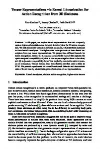
5.4. Computational efficiency The computational efficiency of our method is evaluated regarding both the time cost of the dictionary learning module and the time cost of the feature extraction process. The tests were conducted in MATLAB on a PC with an Intel i5 CPU and 32G memory. Dictionary learning. Algorithm 1 is compared with the K-SVD algorithm for solving (2) and its tensor extensions including K-HOSVD [34] and K-CPD [15].4 The running time is measured on 7.2 × 104 patches sampled from the DynTex++ dataset. The results w.r.t. different patch sizes are plotted in Fig. 1(a). It can be seen that our method is more efficient than K-SVD, K-HOSVD and K-CPD and is scalable to larger patches. Compared with the OMP algorithm used in K-SVD for sparse coding, the thresholding in our method is much more efficient. Meanwhile, the separability of dictionary in our method permits to break down the original problem into three subproblems with reduced dimensions and less variables, which is more computationally efficient and scalable. It is noted that the convergence of Alg. 1 cannot be guaranteed due to the non-convexity of the problem (4). For further understanding the behavior of Alg. 1, we show the objective function value decay over the iteration in Fig. 1(c). Feature extraction. The running time of extracting the proposed descriptor using patch size 7 × 7 is compared to several competitive methods using default parameters, including LBP-TOP, DFS, OTF, and WMFS. Besides, for simulating the case where K-SVD instead of the proposed tensor dictionary learning model is used in our framework, we replace the sparse coding module in our feature extraction by 4 The

K-HOSVD and K-CPD methods are implemented in Matlab with the TPTOOL and PROPACK toolboxes. The code of K-SVD is available on http://www.cs.technion.ac.il/ ronrubin/software.html.

79

OMP (Orthogonal Matching Pursuit) under the dictionary learned by K-SVD and report the resulting time cost. The results w.r.t. different sizes of sequences are shown in Fig. 1(b) under the Logarithm coordinate. Obviously, our method is more efficient and scalable than other compared methods. Such advantages come from both the use of separated 1D convolutions and the use of histogram. The WMFS, OTF, and DFS methods are also filter-based methods, but they compute fractal spectra instead of histograms of filter responses to improve discriminability, which is much more time-consuming. Regardless of the cost of computing fractal spectra, our method still has advantages in computation over OTF, as it employs non-separable 3D filters. The LBP-TOP method is a histogram-based method, in which the computation of local features is accelerated by lookup table. Although it is comparable to our method in computational time, LBP-TOP is inferior regarding accuracy. Remark 3. We replaced our dictionary learning and sparse coding modules by K-SVD, K-HOSVD and K-CPD respectively, and tested the resulting performances on DynTex++. The results are slightly inferior to ours with performance gaps around 0.81%-1.52%. It is also found that using OMP for sparse coding in feature extraction achieved better results than direct filtering with the atoms learned by K-SVD. This is mainly due to the inconsistency between filtering and the K-SVD learning model. 3000

8

1500 1000 500

9 8 7 6 5 4 LBP−TOP DFS OTF WMFS OMP Ours

3 2 1

0 3

4

5

6

7

8

Patch Size

(a)

9

0 0

50

100

150

200

250

Video Size (N × N × N)

(b)

300

350

400

Objective Function Value

Logarithm of Running Time (s)

Training Time (s)

2000

×10 9

10

KSVD K-HOSVD K-CPD Ours

2500

6

4

2

0 0

5

10

15

20

25

Number of Iteration

(c)

Figure 1. Time costs and decay behavior (a) Time cost of dictionary learning; (b) Time cost of feature extraction; (c) Decay behavior of objective function value.

6. Conclusion This paper aims at exploiting sparse representation for DT recognition. We proposed a structured tensor dictionary learning method for extracting local DT patterns, which learns a separable dictionary with orthogonal components from a stack of DT volume patches. The learned atoms are able to characterize the patterns of spatial appearance and temporal dynamics in DT sequences. Benefiting from the separability and orthogonality of dictionary, a fast and scalable numerical algorithm for learning as well as a discriminative and scalable DT descriptor for DT recognition is developed. In the experiments, the proposed DT descriptor

shows noticeable performance improvement in both classification accuracy and time cost over the existing ones. One limit of our method is that the learned atoms cannot be used for multi-scale analysis compared with the multi-scale geometry analysis approaches. Learning multiple dictionaries with different atom sizes can be helpful but is not computationally efficient. In future, we would like to investigate structured dictionary learning under a multi-scale analysis framework. Furthermore, our method can be applied to dynamic scene recognition by combining the learned features into state-of-the-art feature integration frameworks. For example, the sparse coding and dictionary learning can also be applied to global feature integration, sample-level feature refinement, and even classification. By this way we can construct a multi-layer sparse learning architecture for recognizing dynamic scenes, which is also what we would like to pursue in the future.

References [1] M. Aharon, M. Elad, and A. Bruckstein. K-SVD: An algorithm for designing overcomplete dictionaries for sparse representation. IEEE Transactions on Signal Processing, 54(11):4311–4322, 2006. 1, 2, 3 [2] C. Bao, J.-F. Cai, and H. Ji. Fast sparsity-based orthogonal dictionary learning for image restoration. In ICCV, pages 3384–3391. IEEE, 2013. 3 [3] C. Bao, H. Ji, and Z. Shen. Convergence analysis for iterative data-driven tight frame construction scheme. Applied and Computational Harmonic Analysis, 38(3):510–523, 2015. 3 [4] J.-F. Cai, H. Ji, Z. Shen, and G.-B. Ye. Data-driven tight frame construction and image denoising. Applied and Computational Harmonic Analysis, 37(1):89–108, 2014. 3 [5] A. B. Chan and N. Vasconcelos. Classifying video with kernel dynamic textures. In ICPR, pages 1–6, 2007. 2, 5, 6 [6] D. Chetverikov and S. Fazekas. On motion periodicity of dynamic textures. In BMVC, pages 167–176, 2006. 1 [7] D. Chetverikov and R. P´eteri. A brief survey of dynamic texture description and recognition. In Computer Recognition Systems, pages 17–26. Springer, 2005. 2 [8] R. Costantini, L. Sbaiz, and S. Susstrunk. Higher order SVD analysis for dynamic texture synthesis. IEEE Transactions on Image Processing, 17(1):42–52, 2008. 1, 2 [9] K. G. Derpanis, M. Lecce, K. Daniilidis, and R. P. Wildes. Dynamic scene understanding: The role of orientation features in space and time in scene classification. In CVPR, pages 1306–1313. IEEE, 2012. 2 [10] K. G. Derpanis and R. P. Wildes. Dynamic texture recognition based on distributions of spacetime oriented structure. In CVPR, pages 191–198. IEEE, 2010. 1, 2, 5, 6 [11] K. G. Derpanis and R. P. Wildes. Spacetime texture representation and recognition based on a spatiotemporal orientation analysis. IEEE Transactions on Pattern Analysis and Machine Intelligence, 34(6):1193–1205, 2012. 2, 6 [12] G. Doretto, A. Chiuso, Y. N. Wu, and S. Soatto. Dynamic textures. International Journal of Computer Vision, 51(2):91–109, 2003. 1, 5

80

[13] G. Doretto, D. Cremers, P. Favaro, and S. Soatto. Dynamic texture segmentation. In ICCV, pages 1236–1242. IEEE, 2003. 1 [14] G. Doretto, E. Jones, and S. Soatto. Spatially homogeneous dynamic textures. In ECCV, pages 591–602. Springer, 2004. 1, 2 [15] G. Duan, H. Wang, Z. Liu, J. Deng, and Y.-W. Chen. Kcpd: Learning of overcomplete dictionaries for tensor sparse coding. In ICPR, pages 493–496. IEEE, 2012. 2, 7 [16] S. Dubois, R. P´eteri, and M. M´enard. Characterization and recognition of dynamic textures based on the 2d+ t curvelet transform. Signal, Image and Video Processing, pages 1–12, 2013. 2, 7 [17] S. Fazekas and D. Chetverikov. Dynamic texture recognition using optical flow features and temporal periodicity. In International CBMI Workshop, pages 25–32. IEEE, 2007. 1 [18] B. Ghanem and N. Ahuja. Phase based modelling of dynamic textures. In ICCV, pages 1–8. IEEE, 2007. 1, 2 [19] B. Ghanem and N. Ahuja. Maximum margin distance learning for dynamic texture recognition. In ECCV, pages 223– 236. Springer, 2010. 1, 2, 6 [20] B. Ghanem and N. Ahuja. Sparse coding of linear dynamical systems with an application to dynamic texture recognition. In ICPR, pages 987–990. IEEE, 2010. 2 [21] B. S. Ghanem. Dynamic textures: Models and applications. PhD thesis, University of Illinois at Urbana-Champaign, 2010. 1 [22] M. Harandi, C. Sanderson, C. Shen, and B. Lovell. Dictionary learning and sparse coding on grassmann manifolds: An extrinsic solution. In ICCV, pages 3120–3127. IEEE, 2013. 2, 6, 7 [23] S. Hawe, M. Seibert, and M. Kleinsteuber. Separable dictionary learning. In ICPR, pages 438–445. IEEE, 2013. 2 [24] T. Hazan, S. Polak, and A. Shashua. Sparse image coding using a 3d non-negative tensor factorization. In ICCV, volume 1, pages 50–57. IEEE, 2005. 1, 2 [25] H. Ji, X. Yang, H. Ling, and Y. Xu. Wavelet domain multifractal analysis for static and dynamic texture classification. IEEE Transactions on Image Processing, 22(1):286– 299, 2013. 2, 6 [26] A. Mumtaz, E. Coviello, G. R. Lanckriet, and A. B. Chan. Clustering dynamic textures with the hierarchical em algorithm for modeling video. IEEE Transactions on Pattern Analysis and Machine Intelligence, 35(7):1606–1621, 2013. 1, 6 [27] Y. Peng, D. Meng, Z. Xu, C. Gao, Y. Yang, and B. Zhang. Decomposable nonlocal tensor dictionary learning for multispectral image denoising. In ICPR, pages 2949–2956. IEEE, 2014. 2 [28] R. P´eteri and D. Chetverikov. Dynamic texture recognition using normal flow and texture regularity. Pattern Recognition and Image Analysis, pages 223–230, 2005. 1, 2, 6 [29] R. P´eteri, S. Fazekas, and M. J. Huiskes. DynTex : A Comprehensive Database of Dynamic Textures. Pattern Recognition Letters, 31:1627–1632, 2010. 5, 6, 7 [30] R. Polana and R. Nelson. Temporal texture and activity recognition. Springer, 1997. 2

[31] X. Qi, C.-G. Li, G. Zhao, X. Hong, and M. Pietik¨ainen. Dynamic texture and scene classification by transferring deep image features. arXiv preprint arXiv:1502.00303, 2015. 1, 7 [32] A. Ravichandran, R. Chaudhry, and R. Vidal. View-invariant dynamic texture recognition using a bag of dynamical systems. In CVPR, pages 1651–1657. IEEE, 2009. 2, 6 [33] R. Rigamonti, A. Sironi, V. Lepetit, and P. Fua. Learning separable filters. In ICPR, pages 2754–2761. IEEE, 2013. 2 [34] F. Roemer, G. Del Galdo, and M. Haardt. Tensor-based algorithms for learning multidimensional separable dictionaries. In ICASSP, pages 3963–3967. IEEE, 2014. 2, 7 [35] P. Saisan, G. Doretto, Y. N. Wu, and S. Soatto. Dynamic texture recognition. In CVPR, volume 2, pages II–58. IEEE, 2001. 1, 2 [36] R. Sivalingam, D. Boley, V. Morellas, and N. Papanikolopoulos. Tensor sparse coding for region covariances. In ECCV, pages 722–735. Springer, 2010. 1 [37] J. R. Smith, C.-Y. Lin, and M. Naphade. Video texture indexing using spatio-temporal wavelets. In ICIP, volume 2, pages II–437. IEEE, 2002. 1 [38] M. Szummer and R. W. Picard. Temporal texture modeling. In ICIP, volume 3, pages 823–826. IEEE, 1996. 1, 2 [39] X. Wei, H. Shen, and M. Kleinsteuber. An adaptive dictionary learning approach for modeling dynamical textures. In ICASSP, pages 3567–3571, May 2014. 1, 2 [40] R. P. Wildes and J. R. Bergen. Qualitative spatiotemporal analysis using an oriented energy representation. In ECCV, pages 768–784. Springer, 2000. 2 [41] F. Woolfe and A. Fitzgibbon. Shift-invariant dynamic texture recognition. In ECCV, pages 549–562. Springer, 2006. 2, 6 [42] J. Xu, S. Denman, S. Sridharan, C. Fookes, and R. Rana. Dynamic texture reconstruction from sparse codes for unusual event detection in crowded scenes. In J-MRE, pages 25–30. ACM, 2011. 1 [43] Y. Xu, S. Huang, H. Ji, and C. Ferm¨uller. Scale-space texture description on sift-like textons. Computer Vision and Image Understanding, 116(9):999–1013, 2012. 6 [44] Y. Xu, Y. Quan, H. Ling, and H. Ji. Dynamic texture classification using dynamic fractal analysis. In ICCV, pages 1219–1226. IEEE, 2011. 1, 2, 5, 6 [45] L. D. Yangmuzi Zhang, Zhuolin Jiang. Discriminative tensor sparse coding for image classification. In BMVC. BMVA Press, 2013. 1, 2 [46] G. Zhao and M. Pietikainen. Dynamic texture recognition using local binary patterns with an application to facial expressions. IEEE Transactions on Pattern Analysis and Machine Intelligence, 29(6):915–928, 2007. 1, 2, 7 [47] G. Zhao and M. Pietik¨ainen. Dynamic texture recognition using volume local binary patterns. In Dynamical Vision, pages 165–177. Springer, 2007. 2, 5, 6 [48] S. Zubair and W. Wang. Signal classification based on blocksparse tensor representation. In DSP, pages 361–365. IEEE, 2014. 1

81