Dynamic Transmission Scheduling and Link Selection in Mobile Cloud ...

Dynamic Transmission Scheduling and Link Selection in Mobile Cloud Computing Huaming Wu and Katinka Wolter Institut f¨ ur Informatik, Freie Universit¨ at Berlin, Takustr. 9, 14195 Berlin, Germany {huaming.wu,katinka.wolter}@fu-berlin.de

Abstract. Recently, mobile devices have multiple wireless interfaces to use, but how to choose an appropriate network interface? Energy-efficient data transmission is a key issue in mobile cloud computing due to energypoverty of the mobile devices. In this paper, we study an energy-delay tradeoff and address the issue of energy-efficient offloading that migrates data-intensive but delay-tolerant applications from the mobile devices to a remote cloud. Through dynamic scheduling and link selection based on Lyapunov optimization for data transmission between the mobile devices and the cloud, we are able to reduce battery consumption of the mobile devices for transferring large volumes of data. We derive a control algorithm which determines when and on which network to transmit data so that energy-cost is minimized by leveraging delay tolerance. Further, we propose and compare three kinds of transmission schedulers with energyefficient link selection policies under heterogeneous wireless network interfaces (e.g., 3G and WiFi), where the average energy consumption is optimized. Keywords: energy-efficient; transmission scheduling; link selection; optimization; delay-tolerant; mobile cloud computing.

1

Introduction

Mobile cloud computing [1] is emerging as a new computing paradigm that aims to augment resource-poor mobile devices, taking advantage of the abundant resources hosted by clouds. Offloading programs from mobile devices to a remote cloud is becoming an increasingly attractive way to reduce execution time and extend battery life time[2]. It makes running computing/data-intensive applications feasible on resource-constrained mobile devices. Apple’s Siri and iCloud [3] are two examples. However, cloud offloading critically depends on a reliable end-to-end communication and on the availability of the cloud. Access to the cloud is usually influenced by uncontrollable factors, such as the instability and intermittency of wireless networks. Mobile devices often have multiple wireless interfaces, such as 3G/EDGE, 4G LTE and WiFi for data transfer. While in most situations 4G LTE uses most energy and WiFi the least, normally WiFi has the highest bandwidth, 3G/EDGE B. Sericola, M. Telek, and G. Horv´ ath (Eds.): ASMTA 2014, LNCS 8499, pp. 61–79, 2014. c Springer International Publishing Switzerland 2014 

62

H. Wu and K. Wolter

the lowest. However, the bandwidth, the energy-efficiency and even the availability of these networks can vary significantly, such that the stated ordering does not always hold true. Not only the availability and quality of access points (APs) may vary from place to place, but also the uplink and downlink bandwidths fluctuate frequently due to multiple factors such as weather, mobility, building shield and so on [4]. If we can adaptively select one of the available links in every slot, energy consumption may be reduced. Energy consumption in mobile devices has become an important issue for network selection. Gribaudo et. al. [5] developed a framework based on the Markovian agent formalism, which could model the dynamics of user traffic and the allocation of the network radio resources. Rahmati et. al. [6] suggested on-thespot network selection by examining tradeoff between energy consumption for WiFi search and transmission efficiency when the WiFi network was intermittently available. In [7], a power control scheme suitable for a multi-tier wireless network was presented. It maximizes the energy-efficiency of a mobile device transmitting on several communication channels while at the same time ensuring the required minimum quality of service. More recently, “delayed” offloading has been proposed: if there is no WiFi available, traffic can be delayed up to some chosen deadline [8]. Some studies like [9] and [4], suggested energy-efficient delayed network selection by exploring the tradeoff between transmit power of heterogeneous network interfaces (e.g., 3G, WiFi) and transmission delay. Many mobile applications are dealing with video, audio, sensor data, or are accessing large databases on the Internet. Delay-tolerant applications are less sensitive to network delays. Participatory sensing applications are a good example of data-intensive but delay-tolerant applications. Participatory sensing is the collective sampling of sensor data by a number of sensor nodes. This creates a body of knowledge on parameters such as personal resource consumption, dietary habits and urban documentation [9]. Data is uploaded from a smartphone to a back-end cloud server either through the cellular network or any available WiFi network. Some of the sensor information is not time-critical and its submission to the server may be delayed until the device enters an energy-efficient network. Users can browse or search the obtained archives through a website at the server side. In this paper, we address the operation of a mobile user terminal equipped with multiple radio access technologies. We focus on energy-efficient offloading of delay-tolerant data to a remote cloud. To this end, we propose a framework based on Lyapunov optimization and contribute the following: (i) minimization of the average energy consumption for the link selection and transmission scheduling problem, and (ii) formulating a number of transmission schedulers when using 3G and WiFi interfaces to transmit data. The remainder of this paper is organized as follows. Section 2 briefly introduces the link selection problem in mobile cloud computating systems. Section 3 analyzes the energy-delay tradeoff by using Lyapunov optimization. Three kinds of transmission schedulers are proposed and investigated in Section 4. Section 5 gives some simulation results. Finally, the paper is concluded in Section 6.

Dynamic Transmission Scheduling and Link Selection

2

63

Problem Formulation

We provide a brief introduction of the studied adaptive link selection problem and consider a Markovian queueing model for dynamic transmission scheduling and link selection in mobile cloud computing systems. 2.1

Multiple Wireless Interfaces

Mobile devices usually have multiple wireless interfaces that can be used for data transfer, such as EDGE (Enhanced GPRS), 3G, WiFi and so on. The time intervals of cellular connectivity (EDGE or 3G) are usually much longer than for WiFi. Especially, EDGE has very high coverage. In addition, the data rates differ significantly (from hundreds of Kbps for EDGE, to a few Mbps for 3G, to ten or more Mbps for WiFi). The achievable data rate for different radio transmission depends on the environment and can vary widely. It is sometimes far below the nominal value. Also energy-efficiency of the different technologies is different. The energy usage for transmitting a fixed amount of data can differ by an order of magnitude or more [9]. In general, the WiFi interface is more energy-efficient than the cellular interface, and data transmission using a good connection requires much less energy than under bad conditions [4]. Thus, offloading large data items from a mobile device to the cloud using WiFi can be more energy-efficient than using cellular radio, but WiFi connections are not always available. Therefore it must be decided when to transmit data and across which network interface. However, this decision is not easy to take since we know neither the future availability of APs nor their transmission quality. 2.2

Adaptive Link Selection

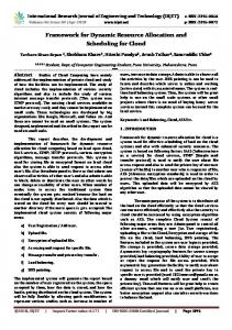
The problem when to transmit data and which mobile interface to use can be formulated as an adaptive link selection problem as depicted in Fig. 1. Given a set of available links with energy information, AP availability information as obtained from traces and data system queues, determine whether to use any of the available links (the appropriate network interface) to transfer data, while keeping the transmission delay bounded [9]. In Fig. 1, the 3G interface is chosen for data transfer. The mobile device selects the link with the best connection quality by running a series of probe-based tests to the cloud. Even after a particular link is selected, the connectivity can still be unstable as it is affected by user mobility, limited coverage of the WiFi APs and other factors. Because it sacrifices delay for energy, the problem of link selection and transmission scheduling for delay-tolerant applications can be naturally formulated using an optimization framework. Suppose there are M channels available, let Bj (t) denote the bandwidth between the mobile device and the cloud in time slot t when using channel j, where j ∈ {1, · · · , M }. Let bj (t) or ˆbj (α(t)) denote the amount of data transmitted over channel j between the mobile device and the cloud in slot t. It is determined by a

64

H. Wu and K. Wolter New Arrivals

System Queue

APs Availability from Traces

Energy Info

Adaptive Link Selection Algorithms

EDGE

3G

LTE

WLAN 1

WLAN n

Fig. 1. A mathematical model of adaptive link selection

transmission decision α(t), which is the choice made in slot t, either to transmit data over channel j or not to transfer, and can be expressed as:  Bj (t) · τ, if α(t)=“Transmit over channel j”, ˆ bj (t) = bj (α(t)) = (1) 0, if α(t)=“Idle”, where α(t)=“Idle” means that no transmission takes place in slot t and τ is the time duration that the interface is on. For convenience, τ is assumed to be a constant, which is based on the bandwidth estimation and should neither too large to too small [4]. We denote the energy consumption caused by data transmission on the mobile ˆ device in time slot t as E(t) = E(α(t)), which depends on the current link bandwidth and the transmission decision α(t). Over a long time period T , the T −1 M total amount of transmitted data is t=0 j=1 bj (t), correspondingly, the total energy consumptionof the mobile device for transmitting such an amount of data T −1 E(t). can be denoted as t=0 Suppose there are N queues of data to be sent from the the mobile device to the cloud, and we define the vector of current queue backlogs by:   Q(t) = Q1 (t), Q2 (t), · · · , QN (t) , ∀t ∈ {0, 1, · · · , T − 1}, (2) where the queues are maintained in the mobile device’s memory and for each queue i, Qi (t) represents its queue backlog of data to be transmitted from the mobile device to the cloud at the beginning of time slot t. Further, let Ai (t) denote the amount of newly arriving data added to each queue i in time slot t. We assume that each random variable Ai (t) is i.i.d. over time slots with expectation E{Ai (t)} = λi . We call λi the arrival rate to queue i. Therefore, the queue length of queue i in time interval t + 1, i.e., Qi (t + 1) has the following dynamics:   Qi (t+1) = max Qi (t)−bi (t), 0 +Ai (t), ∀i ∈ {1, 2, · · · , N }, ∀t ∈ {0, 1, · · · , T −1}. (3)

Dynamic Transmission Scheduling and Link Selection

65

Given this notation, we can formally state the queueing constraint that is imposed on our adaptive link selection algorithm. We require all the queues to be stable in the time average sense, i.e., T −1 N 1  ¯ Q  lim sup E{Qi (t)} < ∞, T →∞ T t=0 i=1

(4)

the stability constraint ensures that the average queue length is finite and we should not always defer the transmission. While maintaining a stable queue we seek to design an adaptive link selection algorithm and dynamic transmission scheduling such that the time-averaged expected transmission energy is minimised [9]: T −1

 ¯  lim sup 1 min E E{E(t)} , T →∞ T t=0

(5)

where the required transmission energy E(t) depends on the selected link for transmission during slot t.

3

Energy-Delay Tradeoff

In this section, an optimization model is formulated, with the objective of minimizing the average energy consumption subject to a stability constraint on the queue of data to be transmitted. 3.1

Problem Analysis Using Lyapunov Optimization

To solve the adaptive link selection problem we employ a Lyapunov optimization framework, which enables us to derive a control algorithm that determines when and on which network to transmit our data such that the total energy-cost is minimized. This optimization is not strict with respect to transmission delay. For each slot t, we define a Lyapunov function [10] as: N

1 2 L(Q(t)) = Q (t), 2 i=1 i

(6)

which represents a scalar measure of queue length in the network. We then define the Lyapunov drift as the change in the Lyapunov function from one time slot to the next: N  1  2 Q (t + 1) − Q2i (t) L(Q(t + 1)) − L(Q(t)) = 2 i=1 i

= ≤

N

2 1   max[Qi (t) − bi (t), 0] + Ai (t) − Q2i (t) 2 i=1 N  A2 (t) + b2 (t) i

i=1

i

2

+

N  i=1

Qi (t)[Ai (t) − bi (t)].

(7)

66

H. Wu and K. Wolter

The conditional Lyapunov drift Δ(Q(t)) is the expected change in the Lyapunov function over one time slot, given that the current state in time slot t is Q(t). That is:  Δ(Q(t)) = E L(Q(t + 1)) − L(Q(t))|Q(t) .

(8)

From (7), we have that for a general control policy Δ(Q(t)) satisfies: 

 

N N N A2i (t) + b2i (t) Δ(Q(t)) ≤ E |Q(t) + Qi (t)λi − E Qi (t)bi (t)|Q(t) (9) , 2 i=1 i=1 i=1 where we have used the assumption that arrivals are i.i.d. over slots and hence independent of current queue backlogs, so that E{Ai (t)|Q(t)} = E{Ai (t)} = λi . Let C be a finite constant that bounds the first term on the right-hand-side of (9), so that for all t, all possible Q(t) and all possible transmission decisions we have:  N 2   N  N   2 E

 Ai (t) + bi (t) i=1

2

|Q(t)

=

 2  2 1 1 E Ai (t) + E bi (t)|Q(t) 2 2 i=1 i=1

≤ C.

(10)

 N 2 There exist constants A2max and b2max that satisfy the conditions: E i=1 Ai (t)   N 2 ≤ b2max , where Amax ≥ Ai (t) represents the ≤ A2max and E i=1 bi (t)|Q(t) maximum amount of data that can arrive per time slot, and bmax ≥ bi (t) denotes the maximum amount of data that can be transmitted via the wireless network in a time slot. Hence, we have C = 12 (A2max + b2max ). To stabilize the data queue by making sure that there is a balance of arriving data and transmitted data, while minimizing the time-averaged energy E(t), we incorporate the expected energy consumption over one slot t. It can be designed to make transmission decisions that greedily minimize a bound on the following drift-plus-penalty term in each slot t [10]: Δ(Q(t)) + V E{E(t)|Q(t)},

(11)

where V ≥ 0 is a control parameter that represents an “importance weight” in deciding relative importance among queue backlog, estimated rate, and energy cost. In other words, V can be thought of as a threshold on the queue backlog beyond which the control algorithm decides to transmit, so V controls the energydelay tradeoff [9]. From (9) and (10) we have: Δ(Q(t)) + V E{E(t)|Q(t)} ≤ C +

N 

Qi (t)λi + V E{E(t)|Q(t)} − E

i=1

= C+

 N

 Qi (t)ˆ bi (α(t))|Q(t)

i=1

N 

  N   Qi (t)λi + E V E(t) − Qi (t)ˆ bi (α(t)) | Q(t) .

i=1

i=1

(12)

Dynamic Transmission Scheduling and Link Selection

67

Using the concept of opportunistically minimizing an expectation, the optimization of the right-hand-side of (12) is accomplished by greedily minimizing the following term: N

 Qi (t)ˆbi (α(t)) , arg min V E(t) − α(t)

(13)

i=1

where we choose the transmission decision α(t) that will minimize (13). N We denote a decision function as d(t) = V E(t) − i=1 Qi (t)ˆbi (α(t)), which is the decision results that depends on the current link bandwidth and the transmission decision α(t). In order to understand the intuition behind this decision, we would like to see when d(t) can have a low value. 1. Link with a Good Quality: d(t) can be small when the link has a high estimated rate. It makes sense that we would like to use any high-quality link to transfer data over a low-quality link. 2. Queue Backlog is High: d(t) can achieve a low-value if the queue backlog Q(t) is high. This is also intuitive: when data has been in the queue for long, there should be a higher incentive to transmit. 3. Link Energy Cost is Low: d(t) is small when the energy cost E(t) of a link is low (e.g., a WiFi link). Such a link should be preferred over a high-energy cellular link [9]. In other words, the link selection model based on Lyapunov optimization defers transmission until good-quality and low-energy links become available, unless the queue backlog is too high. Further, considering the decision α(t), the decision function d(t) can be denoted as:  V Ei (t) − Qi (t)bi (t), if α(t)=“Transmit over channel i”, (14) d(t) = 0, if α(t)=“Idle”. 3.2

Performance Bounds

For any control parameter V > 0, we assume that the data arrival rate λi is strictly within the network capacity region, which is defined as the region that can be achieved by the mobile device in communication networks [9]. We can achieve a time-averaged energy consumption and queue backlog satisfying the following constraints [11]: T −1 C 1  E{E(t)} ≤ E ∗ + , E¯ = lim sup V T →∞ T t=0

(15)

T −1  N  ¯ C + V (E ∗ − E) ¯ = lim sup 1 Q , E{Qi (t)} ≤ ε T →∞ T t=0 i=1

(16)

68

H. Wu and K. Wolter

where ε > 0 is a constant denoting the distance between arrival pattern and the capacity region boundary [9], E ∗ is a theoretical lower bound on the timeaveraged energy consumption using any control policy that achieves queue stability. Proof. Because the transmission decision α(t) minimizes the right-hand-side of the drift-plus-penalty in inequality (12), in every slot t (given the observed Q(t)), we have: N   ˆ ∗ (t))|Q(t) + Qi (t)λi Δ(Q(t)) + V E{E(t)|Q(t)} ≤ C + V E E(α i=1



N ∗ ˆ −E Qi (t)bi (α (t))|Q(t) ,

(17)

i=1

where α∗ (t) is any other (possibly randomized) transmission decision that can be made in slot t. Fixing any value ε > 0 in the capacity region boundary further yields: N N     ˆ ∗ (t))|Q(t) + Δ(Q(t))+V E{E(t)|Q(t)} ≤ C + V E E(α Qi (t)λi − Qi (t)(λi + ε) i=1

  ˆ ∗ (t))|Q(t) −ε = C + V E E(α

N 

i=1

Qi (t).

(18)

i=1

Taking expectations for (18) with respect to Q(t) and using the law of iterated expectations, yields: E{L(Q(t + 1))} − E{L(Q(t))} + V E{E(t)} ≤ C + V E ∗ − ε

N 

E{Qi (t)},

(19)

i=1

 ˆ ∗ (t)) . where E ∗  E E(α Summing the above inequality over t ∈ {0, 1, · · · , T − 1} for some positive integer T , yields: E{L(Q(T ))}−E{L(Q(0))}+V

T −1 

E{E(t)} ≤ CT +V T E ∗ −ε

t=0

N T −1  

E{Qi (t)}. (20)

t=0 i=1

Then, dividing (20) by V T and after a simple manipulation we obtain: T −1 ε C 1  + E∗ − E{E(t)} ≤ T t=0 V

T −1 N t=0

i=1

VT

E{Qi (t)}

−

E{L(Q(T ))} E{L(Q(0))} + . VT VT (21)

Since the Lyapunov function is non-negative by definition and so is E ∗ , neglecting that we subtract non-negative quantities in (21) yields: T −1 E{L(Q(0))} 1  C . E{E(t)} ≤ P ∗ + + T t=0 V VT

(22)

Dynamic Transmission Scheduling and Link Selection

69

Similarly, dividing (20) by εT , and after rearranging terms we obtain: T −1 N C + V (E ∗ − 1  E{Qi (t)} ≤ T t=0 i=1

1 T

T −1 t=0

E{E(t)})

ε

+

E{L(Q(0))} . (23) εT

Finally, taking a lim sup as T → ∞ in inequalities (22) and (23), we can derive (15) and (16), respectively.  It can be seen that (15) and (16) demonstrate an [O(1/V ), O(V )] tradeoff between energy consumption and delay. We can achieve an average energy con¯ arbitrarily close to E ∗ while maintaining queue stability. However, sumption E this is achieved at the expense of a larger delay because the average queue back¯ increases linearly with V . Choosing a large value of V can thus push the log Q average energy arbitrarily close to its optimal value. However, this comes by sacrificing average queue backlog or average delay that is O(V ) [10]. A good V value is one that achieves a good energy and delay tradeoff, where a unit increase ¯ with consistently growing delays [9]. In in V yields a very small reduction in E mathematical terms we can choose a k < 0 that satisfies:  C d(E ∗ + C/V ) ≥ k =⇒ V ≥ , (24) dV −k ¯ curve. where k is the slope of E

4

Performance Analysis Models

To understand this link selection algorithm, we consider the two most prominent networks: WiFi and 3G. Typically, the WiFi interface is much more energyefficient, but its availability is limited while the 3G network is available almost everywhere. Besides, channel quality can be affected by environmental factors and interference. The channel bandwidth can be reduced due to competing users in the same cells. Therefore, for data-intensive but delay-tolerant applications, we can save energy by delaying transmissions until a good-quality or a low-energy interface such as WiFi becomes available, unless the queue backlog is too high. 4.1

Bandwidth Estimation and Energy Models

Since our transmission scheduling model uses the knowledge of current states (i.e, the current network bandwidth is supposed to be known), it closely depends on the bandwidth estimation. We use a predictor proposed in [12], which considers the classical bandwidth predictors (such as Last value, Mean filter, Network weather service forecaster, etc.) synthetically. The framework unifies such decision models by formulating the problem as a statistical decision problem that can either be treated “classically” or using a Bayesian approach. The experimental result shows that the Bayes strategy performs significantly better than the traditional predictors. Thus, this prediction model is more general and

70

H. Wu and K. Wolter Table 1. Energy model for 3G and WiFi networks Items 3G Ramp and Transfer Energy R(x) 0.025x + 3.5 Tail power P 0.62J/s Tail time T 12.5s

WiFi 0.007x + 5.9 NA NA

could be used by our offloading system. Further, we assume that the network bandwidth is constant in one time slot. Table 1 lists the measured energy consumption models according to [13]. The energy needed to transmit x bytes of data over the cellular network can be split into three components: ramp energy, transmission energy and tail energy. R(x) denotes the sum of the ramp and the transfer energy to send x KB, P denotes the tail power and T denotes the tail time. Obviously, the energy consumption depends on the type of interface that is selected. For the 3G interface, the sum of the ramp and the transfer energy is R(x) = 0.025x + 3.5. After transmitting a packet, instead of transitioning from high to low power state, the 3G interface spends substantial time in the high state, which incurs considerable energy, referred to as the tail energy. For the WiFi interface, the sum of the ramp and the transfer energy is R(x) = 0.007x + 5.9, and the tail energy is zero. Using WiFi, the data transfer itself is significantly more efficient than using the 3G connection for all transfer sizes. In addition to the transfer cost, the total energy to transmit a packet also depends on the time that the interface is on. Therefore, the energy consumption for the 3G and WiFi interfaces in time slot t can be expressed as follows:

4.2

E3G (t) = 0.025 · b3G (t) + 3.5 + 0.62 · 12.5,

(25)

EWiFi (t) = 0.007 · bWiFi (t) + 5.9.

(26)

Transmission Scheduler I (N = M )

The model of the transmission scheduler I for only one queue of arriving jobs is depicted in Fig. 2. The arrival vector A(t) is assumed to be i.i.d over the time slot and E{A(t)} = λ. We take decisions of transmission scheduling according to the estimate of the current network bandwidth. In Fig. 2, “B3G (t)” represents the estimated 3G bandwidth in slot t, “BWiFi (t)” represents the estimated WiFi bandwidth and “Idle” denotes that no transmission takes place in time slot t. If B3G (t) is larger than BWiFi (t), the mobile device will be linked to the 3G interface in time slot t to transmit data, otherwise it will be linked to the WiFi interface. The decision criterion can be denoted as max{B3G (t), BWiFi (t)}. Therefore, the bandwidth of the selected interface is as follows:  B3G (t), if B3G (t) > BWiFi (t), B(t) = (27) BWiFi (t), otherwise.

Dynamic Transmission Scheduling and Link Selection

71

B3G (t ) max ^ B3G (t ), BWiFi (t )` x

Q(t)

A(t )

BWiFi (t )

x arg min ª¬VE (t )  Q(t )bˆ D (t ) º¼ D (t )

b(t)

Idle

Fig. 2. Model of transmission scheduler I

According to the Lyapunov optimization, the minimization of the average energy consumption is accomplished by greedily minimizing the following criterion:

(28) arg min V E(t) − Q(t)ˆb(α(t)) . α(t)

Denoting the decision function as d(t) = V E(t) − Q(t)ˆb(α(t)), when considering the transmission decision α(t) we have:  V E(t) − Q(t)B(t) · τ, if α(t) = “transmit”, d(t) = (29) 0, if α(t) = “idle”, where α(t) ∈ {“transmit” and “idle”}, taking on two possible values and ⎧ ⎨ E3G (t), if α(t) = “transmit” and B3G (t) > BWiFi (t), E(t) = EWiFi (t), if α(t) = “transmit” and B3G (t) ≤ BWiFi (t), ⎩ 0, if α(t) = “idle”. If the transmission decision is α(t) = “transmit”, we choose to transfer data according to the current channel bandwidth. If α(t) = “idle”, no data is transmitted in slot t, so E(t) = 0 and b(t) = 0, and then we have d(t) = 0. Therefore, transmission takes place only if V satisfies: V E(t) − Q(t)ˆb(α(t)) < 0. This happens when the bandwidth is high, making a large ˆb(α(t)), or the queue Q(t) is already congested in time slot t. Over time, the queuing dynamic is given by: Q(t + 1) = max[Q(t) − b(t), 0] + A(t),

∀t ∈ {0, 1, · · · , T − 1}.

(30)

By Little’s Theorem [14], the average delay can be calculated as: ¯ ¯ = Q. D λ

(31)

The disadvantage of transmission scheduler I is that only the estimated bandwidth of 3G and WiFi in time slot t is considered and the energy usage of

72

H. Wu and K. Wolter

3G and WiFi is not taken into account. For example, if B3G (t)=50Kbps and BWiFi (t)=49.99Kbps, since B3G (t) is larger than BWiFi (t) we choose the 3G interface to transmit data, even though it consumes much more energy than WiFi. In this situation we should also consider the energy demand of 3G and WiFi. 4.3

Transmission Scheduler II (N = M )

The model of transmission scheduler II is shown in Fig. 3. There are two links (M = 2) available for selection. We also use one queue (N = 1) to represent data transmission during each slot.

B3G (t )

Q(t )

A(t )

Idle

BWiFi (t )

­b1 (t ) B3G (t ) ˜W ® ¯b2 (t ) 0 2 ª º arg min «VE (t )  Q(t )¦ bˆ j D (t ) » D (t ) j 1 ¬ ¼

­b1 (t ) 0 ® ¯b2 (t ) 0

b(t ) x

­b1 (t ) 0 ® ¯b2 (t ) BWiFi (t ) ˜W

Fig. 3. Model of optimal transmission scheduler II

Using the concept of opportunistically minimizing the expectation, the minimization of average energy consumption is accomplished by greedily minimizing: M

 ˆbj (α(t)) . arg min V E(t) − Q(t) α(t)

(32)

j=1

 ˆ Similarly, let d(t) = V E(t) − Q(t) M j=1 bj (α(t)). Since M = 2, there are three possible results according to the transmission decision of α(t): ⎧ if α(t)=“transmit via 3G”, ⎨ V E3G (t) − Q(t)B3G (t) · τ, (33) d(t) = V EWiFi (t) − Q(t)BWiFi (t) · τ, if α(t)=“transmit via WiFi”, ⎩ 0, if α(t)=“idle”, where α(t) ∈ {“transmit via 3G”, “transmit via WiFi” and “idle”} is the transmission decision in slot t, taking on three possible values. According to (33), we not only consider the estimated bandwidth but also take into account the energy usage of 3G and WiFi in time slot t. We thus compare the above values and choose the transmission decision corresponding to the smallest outcome. The queuing dynamics and the average delay are given by (30) and (31), respectively. If the 3G and WiFi interfaces can be used simultaneously, the model of transmission scheduler II in Fig. 3 can be further extended as in Fig. 4.

Dynamic Transmission Scheduling and Link Selection B3G (t ) ˜W

B3G (t )

Q(t )

BWiFi (t ) ˜W

BWiFi (t )

A(t )

73

3 ª º arg min «VE (t )  Q(t )¦ bˆ j D (t ) » D (t ) j 1 ¬ ¼

x

0

Idle

B3G (t )  BWiFi (t )

b(t )

> B3G (t )  BWiFi (t )@ ˜W

Fig. 4. Model of transmission scheduler II for the combined scheme

Since the combined transmission works just like an extra channel, we have M = 3. Thus, there are four possible results in (32) according to the transmission decision of α(t): d(t) =

⎧ V E3G (t) − Q(t)B3G (t) · τ, if ⎪ ⎪ ⎨ V EWiFi (t) − Q(t)BWiFi if  (t) · τ,  ⎪ V · E3G (t) + EWiFi (t) − Q(t) · B3G (t) + BWiFi (t) · τ, if ⎪ ⎩ 0, if

α(t)=“transmit via 3G”, α(t)=“transmit via WiFi”, α(t)=“transmit via 3G and WiFi”, α(t)=“idle”,

where α(t) ∈ {“transmit via 3G”, “transmit via WiFi”, “transmit via 3G and WiFi”, and “idle”} is the transmission decision in slot t, taking on four possible values. 4.4

Transmission Scheduler III (N = M )

The model of transmission scheduler III is depicted in Fig. 5. To overcome the problem pointed out above and to take more accurate decisions, we divide the data into two queues. The number of channels is equal to the number of queues, that is N = M = 2. Q1 (t )

B3G (t )

A1 (t )

A(t )

Idle

­b1 (t ) B3G (t ) ˜W ® ¯b2 (t ) 0 2 ª º arg min «VE (t )  ¦ Qi (t )bˆi D (t ) » D (t ) i 1 ¬ ¼

­b1 (t ) 0 ® ¯b2 (t ) 0

x

A2 (t )

Q2 (t )

BWiFi (t )

­b1 (t ) 0 ® ¯b2 (t ) BWiFi (t ) ˜W

Fig. 5. Model of transmission scheduler III

It can be seen from Fig. 5 that A1 (t) is only transmitted through the 3G interface while A2 (t) is only transmitted through the WiFi interface. We assume

74

H. Wu and K. Wolter

that A1 (t) and A2 (t) take integer units of packets, the arrival vector A(t) is i.i.d over slot and E{A(t)} = λ. The question whether or not to allocate A(t) to A1 (t) and A2 (t) in equal shares still remains. To analyze this problem, we simplify the model as shown in Fig. 6, such that it involves routing decisions besides scheduling decisions. B3G (t )

A1 (t )

­b1 (t ) B3G (t ) ˜W ® ¯b2 (t ) 0 2 ª º arg min «VE (t )  ¦ Qi (t )bˆi D (t ) » D (t ) i 1 ¬ ¼

Q1 (t )

Idle

x

­b1 (t ) 0 ® ¯b2 (t ) 0

Q2 (t )

A2 (t )

BWiFi (t )

­b1 (t ) 0 ® ¯b2 (t ) BWiFi (t ) ˜W

Fig. 6. Equivalent model of transmission scheduler III

There are two separate queues depicted in Fig. 6, the arrival vectors A1 (t) and A2 (t) are i.i.d over slot, E{A1 (t)} = λ1 and E{A2 (t)} = λ2 . Since A1 (t)+A2 (t) = A(t), according to the property of the Poisson distribution we have: λ1 + λ2 = λ,

(34)

where λ1 = ρλ, λ2 = (1 − ρ)λ, and 0 ≤ ρ ≤ 1 is the ratio of arrival rate to queue 1. There are two extreme cases: when ρ = 0, the mobile device only uses the WiFi interface to transmit data and when ρ = 1, the mobile device only uses the 3G interface. Similarly, using the concept of opportunistic minimization of the expectation, the minimization of the average energy consumption is accomplished by greedily minimizing: 2

 Qi (t)ˆbi (α(t)) . (35) arg min V E(t) − α(t)

2

i=1

Let d(t) = V E(t) − i=1 Qi (t)ˆbi (α(t)). Then there are three possible results according to the transmission decision of α(t) as given by: ⎧ if α(t)=“transmit via 3G”, ⎨ V E3G (t) − Q1 (t)b1 (t), d(t) = V EWiFi (t) − Q2 (t)b2 (t), if α(t)=“transmit via WiFi”, (36) ⎩ 0, if α(t)=“idle”, where α(t) ∈ {“transmit via 3G”, “transmit via WiFi” and “idle”} is the transmission decision in slot t, taking on the three possible values. The amount of data transmitted between the mobile device and the cloud in slot t is as follows: ⎧ if α(t)=“transmit via 3G”, ⎨ {B3G (t) · τ, 0}, {b1 (t), b2 (t)} = {0, BWiFi(t) · τ }, if α(t)=“transmit via WiFi”, ⎩ {0, 0}, if α(t)=“idle”,

Dynamic Transmission Scheduling and Link Selection

75

and the queuing dynamics are given by: Qi (t+1) = max[Qi (t)−bi (t), 0]+Ai (t), ∀i ∈ {1, 2}, ∀t ∈ {0, 1, · · · , T −1}. (37) Similarly, the average delay for this system is: ¯ = Q1 + Q2 . D λ1 + λ2

(38)

Furthermore, the transmission scheduler III can be extended in the same way to more general scenarios as depicted in Fig. 1, where several traffic queues can be concurrently distributed over several communication channels.

5

Simulation Results

As for parameter setting, we assume that data arrivals follow Possion Process with λ = 4 packets/minute and the size of each packet is 100 KB. Suppose that the network bandwidths stay the same during each time slot. Our algorithms are simulated in 1,000 time slots for each of the V value ranging from 1 to 300. We study the impact of parameter V on time-averaged energy consumption, queue backlog, delay and transmit data. The energy consumption models are according to (25) and (26) for the 3G and WiFi interfaces, respectively. We first estimate the achievable network bandwidth B(t) at the beginning of every time slot t. Since data communication time between the mobile device and the cloud depends on the network bandwidth and the bandwidth of wireless LAN is remarkably higher than the bandwidth provided by radio access on a mobile device, we suppose that the bandwidth for the 3G interface follows a uniform distribution on [1, 100] KB/s and the bandwidth for the WiFi interface follows a uniform distribution on the interval [1, 300] KB/s. We set the length of each slot τ = 60, and the bandwidth in the corresponding time slot t is used for every 60 seconds. It can be seen from Fig. 7 (transmission scheduler I, refer to Fig. 2) that the time-average energy consumption and transmit data fall quickly at the beginning and then tend to descend slowly while the time-average queue backlog grows linearly with V . This finding confirms the [O(1/V ), O(V )] tradeoff as captured in (15) and (16). According to different delay-tolerant and data-intensive applications, we can adjust the value of V to control the energy-delay tradeoff. Especially, there exists a sweet spot of V , and at this point, the marginal energy conservation is not worth the consistently growing delay with increasing of V . For example, when V increases from 100 to 200, it shows a negligible decrease of the average energy consumption while the average delay increases significantly, thus we should not trade energy with delay. Further, according to (24), the slope of the curve is k ≈ 0 at this point. The numerical results of using transmission scheduler II are depicted in Fig. 8. We compare the scheme that combines 3G and WiFi (refer to Fig. 4) with the one that transmit separately (refer to Fig. 3). It can be seen that the average

76

H. Wu and K. Wolter Transmission scheduler I (λ=4) 100

90

Energy consumption [J/min] Queue backlog [Packets] Transmit data [Packets]

80

70

60

50

40

30

20

10

0

0

20

40

60

80

100

120

140

160

180

200

V

Fig. 7. The impact of V on time-averaged energy consumption, queue backlog and transmit data for transmission scheduler I

number of transmitted packets and average delay in both schemes almost coincide with each other while the combined scheme achieves a lower average energy consumption than both individual schemes when the control factor V is small (e.g., V ≤ 50). Transmission scheduler II (λ=4) 120 Energy consumption (combined) Delay (combined) Transmit data (combined) Energy consumption Delay Transmit data

100

80

60

40

20

0

0

50

100

150

V

Fig. 8. Comparison of different schemes for transmission scheduler II

The numerical results of using transmission scheduler III for the scenario (refer to Fig. 6) are depicted in Figs. 9-11. It is known that when ρ = 0 (ρ is defined before as the dispatching ratio of arrival rate to queue 1), the mobile device only uses the WiFi interface to transmit data and when ρ = 1, it only uses the 3G interface. As shown in Fig. 9, when V is small, it has the minimum energy consumption when only using 3G for data transfer, while it has the maximum energy consumption when only

Dynamic Transmission Scheduling and Link Selection

77

Transmission scheduler III (λ=4) 90

ρ=0 ρ=0.25 ρ=0.5 ρ=0.75 ρ=1

80

Average Energy (J/Minute)

70

60

50

40

30

20

10

0

0

20

40

60

80

100

120

140

160

180

200

V

Fig. 9. The impact of V on time-averaged energy consumption Transmission scheduler III (λ=4) 250

Average delay (Minutes)

200

ρ=0 ρ=0.25 ρ=0.5 ρ=0.75 ρ=1

150

100

50

0

0

50

100

150

200

250

300

V

Fig. 10. The impact of V on time-averaged delay

using WiFi. The average energy increases with the increase of ρ when V ≤ 37. However, when V arrives to a certain value (V ≈ 37), the scheme that only uses WiFi for data transfer has the minimum energy consumption while the one that only uses 3G has the maximum energy consumption. The time-averaged energy consumption increases with the increment of ρ when V > 37. Therefore, the energy consumption for such a transmission scheduler closely depends on the value of ρ. The impact of V on the time-averaged delay is shown in Fig. 10. It is found that the average delay is minimal when only using WiFi to transmit data. With the increase of ρ, the average delay at first increases, but it then decreases after ρ arrives at some value, for example, the average delay is smaller for ρ = 1 than for ρ = 0.75.

78

H. Wu and K. Wolter Transmission scheduler III (λ=4) 100

ρ=0 ρ=0.25 ρ=0.5 ρ=0.75 ρ=1

Average Transmit Data (Packages)

90

80

70

60

50

40

30

20

10

0

0

50

100

150

200

250

300

V

Fig. 11. The impact of V on time-averaged transmit data

The impact of V on time-averaged transmitted data is depicted in Fig. 11. It can be seen that when V is small, the average transmit data decreases with the increment of ρ, thus the mobile device can transfer the largest amount of data when only using the WiFi interface to transmit data due to its high bandwidth. However, when V is large, the average transmitted data is almost the same and does not change with increasing of V .

6

Conclusion and Future Work

In this paper, we present a fundamental approach for designing an online algorithm for the energy-delay tradeoff in “delayed” mobile data offloading through the Lyapunov optimization framework. Considering the changing landscape of network connectivity, the problem of link selection and data transmission scheduling can be formulated as an optimization problem, in which a significant amount of energy can be saved without sacrificing on the transmission delay too much. Three types of transmission schedulers are proposed and compared based on simulation results. These energy-efficient transmission schedulers consider several factors: data backlog, channel quality and energy consumption of the wireless interface, when making transmission decisions. They will choose to transmit data when the connectivity is good enough or when the queues in the mobile device are congested. So far the validation of the approach is based on simulation under simplifying assumptions. For future work, validation based on real workloads and more realistic application examples will be provided to gain insights about efficiency of the proposed algorithm in practice. Besides, a mobile-cloud offloading middleware will be developed to apply those schedulers to reduce energy consumption for delay-tolerant applications on mobile devices.

Dynamic Transmission Scheduling and Link Selection

79

References 1. Armbrust, M., Fox, A., Griffith, R., Joseph, A., Katz, R., Konwinski, A., Lee, G., Patterson, D., Rabkin, A., Stoica, I., Zaharia, M.: Above the Clouds: A Berkeley View of Cloud Computing. Technical Report No. UCB/EECS-2009-28.University of California at Berkley, USA (2009) 2. Niu, D.: Gearing Resource-Poor Mobile Devices with Powerful Clouds: Architectures, Challenges, and Applications. IEEE Wireless Communications 20(3), 14–22 (2013) 3. Apple Company, http://www.apple.com/icloud/ 4. Shu, P., Liu, F., Jin, H., Chen, M., Wen, F., Qu, Y., Li, B.: eTime: Energy-Efficient Transmission between Cloud and Mobile Devices. In: Proc. of IEEE Infocom, pp. 195–199. IEEE Press, New York (2013) 5. Gribaudo, M., Manini, D., Chiasserini, C.: Studying Mobile Internet Technologies with Agent based Mean-Field Models. In: Dudin, A., De Turck, K. (eds.) ASMTA 2013. LNCS, vol. 7984, pp. 112–126. Springer, Heidelberg (2013) 6. Rahmati, A., Zhong, L.: Context-for-Wireless: Context-Sensitive Energy-Efficient Wireless Data Transfer. In: Proc. of the 5th International Conference on Mobile Systems, Applications and Services, pp. 165–178. ACM, New York (2007) 7. Galinina, O., Trushanin, A., Shumilov, V., Maslennikov, R., Saffer, Z., Andreev, S., Koucheryavy, Y.: Energy-Efficient Operation of a Mobile User in a Multi-tier Cellular Network. In: Dudin, A., De Turck, K. (eds.) ASMTA 2013. LNCS, vol. 7984, pp. 198–213. Springer, Heidelberg (2013) 8. Mehmeti, F., Spyropoulos, T.: Performance Analysis of On-the-Spot Mobile Data Offloading. In: Proc. of IEEE Globecom. IEEE Press, New York (2013) 9. Ra, M., Paek, J., Sharma, A., Govindan, R., Krieger, M., Neely, M.: Energy-Delay Tradeoffs in Smartphone Applications. In: 8th International Conference on Mobile Systems, Applications, and Services, pp. 255–270. ACM, New York (2010) 10. Neely, M.J.: Stochastic Network Optimization with Application to Communication and Queueing Systems. In: Synthesis Lectures on Communication Networks, vol. 3(1), pp. 1–211. Morgan & Claypool Publishers (2010) 11. Georgiadis, L., Neely, M.J., Tassiulas, L.: Resource Allocation and Cross-Layer Control in Wireless Networks. Now Publishers Inc. (2006) 12. Wolski, R., Gurun, S., Krintz, C., Nurmi, D.: Using Bandwidth Data to Make Computation Offloading Decisions. In: IEEE International Symposium on Parallel and Distributed Processing, IPDPS 2008, pp. 1–8. IEEE Press, New York (2008) 13. Balasubramanian, N., Balasubramanian, A., Venkataramani, A.: Energy Consumption in Mobile Phones: A Measurement Study and Implications for Network Applications. In: 9th ACM SIGCOMM Conference on Internet Measurement Conference, pp. 280–293. ACM, New York (2009) 14. Bertsekas, D.P., Gallager, R.G., Humblet, P.: Data Networks. Prentice-Hall International, New Jersey (1992)