Dynamic VaR models and the Peaks over Threshold method ... - UniTN

Department of Economics

Dynamic VaR models and the Peaks over Threshold method for market risk measurement: an empirical investigation during a financial crisis Marco Bee, Fabrizio Miorelli

n. 9/2010

Dynamic VaR models and the Peaks over Threshold method for market risk measurement: an empirical investigation during a financial crisis Marco Bee

Fabrizio Miorelli June 14, 2010

Abstract This paper presents a backtesting exercise involving several VaR models for measuring market risk in a dynamic context. The focus is on the comparison of standard dynamic VaR models, ad hoc fat-tailed models and the dynamic Peaks over Threshold (POT) procedure for VaR estimation with different volatility specifications.

We

introduce three different stochastic processes for the losses: two of them are of the GARCH-type and one is of the EWMA-type. In order to assess the performance of the models, we implement a backtesting procedure using the log-losses of a diversified sample of 15 financial assets. The backtesting analysis covers the period March 2004 - May 2009, thus including the turmoil period corresponding to the subprime crisis. The results show that the POT approach and a Dynamic Historical Simulation method, both combined with the EWMA volatility specification, are particularly effective at high VaR coverage probabilities and outperform the other models under consideration. Moreover, VaR measures estimated with these models react quickly to the turmoil of the last part of the backtesting period, so that they seem to be efficient in high-risk periods as well.

Keywords: Market risk, Extreme Value Theory, Peaks over Threshold, Value at Risk, Fat tails.

hello

1 Introduction Market risk was the earliest type of risk systematically tackled both by practitioners and academics. Massive developments in the methodology have been triggered by the release of the Market Risk Amendment by the Bank of International Settlement (BIS, 1996). In order to keep a certain capital buffer against adverse market movements, banks and financial institutions with relevant trading activity have to measure regularly the exposure on the financial assets held in their trading portfolios. This exposure has to be converted in a monetary amount, the so-called regulatory capital required against market risk. Standard approaches to market risk measurement are mostly based on the normality assumption, which is often inadequate from the empirical point of view. A well-known measure of market risk, used both for internal risk management and regulatory purposes, is the so-called Value-at-Risk (VaR), which estimates, given a certain time horizon, the maximum loss that a bank is going to suffer with a certain probability level. The VaR, originally proposed by J.P. Morgan (RiskMetrics, 1996), has become a standard tool in market risk management. Employing the VaR parametric setup requires various statistical assumptions. A commonly accepted starting point is that, when dealing with the production of short-term VaR estimates, a dynamic approach is preferable, because it allows to capture the empirical properties of the loss time series. In this case, the primary concern is the choice of an accurate econometric model that takes into account some stylized facts of financial time series. Among them (see, for example, Cont, 2001), the main features considered in this article are heteroskedasticity, persistence and fat tails. The first two are strictly connected with the empirical autocorrelation function of squared losses, which is typically significantly positive for a long time, while the third one is observed both in the filtered conditional loss distribution and in the unconditional loss distribution. Many VaR models try to incorporate one or more of these stylized facts. The earliest dynamic VaR approaches assemble conditional volatility models like ARCH (Engle, 1982) or GARCH (Bollerslev, 1986), which directly model the persistence in squared returns/losses, with the standard normal distribution. Although they usually fit the data reasonably well, the normality assumption is generally a cause of VaR underestimation, because the filtered conditional loss distribution, i.e. the distribution of standardized losses, is often heavier-tailed than the normal. Thus, especially at high coverage levels, these models are quite inadequate. An obvious solution (see, for example, Angelidis et al., 2004; Hung et al., 2008) consists in fitting a distribution with tails fatter than the normal: the data generating processes range from the simple standardized Student-t or Generalized Error Distribution (GED), to the more complex Edgeworth-Sargan distribution (see Baixauli and Alvarez, 2006). From a theoretical point of view, each of these models may suit the filtered loss data better than the normal distribution. However, they are based on a priori hypotheses on the data-generating process. This fact, which entails some lack of generality, is considered their major drawback, although the performance may be good in specific cases. Recently, there have been a lot of efforts towards the implementation of techniques and methods belonging to the field of Extreme Value Theory (EVT). In particular, the Peaks Over Threshold (POT)

1

method seems to be the most effective way of applying EVT to VaR estimation: here, we refer mainly to the dynamic POT approach developed in McNeil and Frey (2000), Fernandez (2003), and Battacharya and Ritolia (2008). This procedure allows to simultaneously take into account persistence in squared returns/losses, heteroskedasticity and fat tails. Roughly speaking, it applies the traditional POT framework (Embrechts et al., 1997; McNeil and Saladin, 1997) to the GARCH residuals or, more generally, to any volatility-filtered loss time series. The main advantages of the approach are generality, strong theoretical basis and acceptable computational tractability, as well as accuracy when dealing with fat-tailed data. The analysis presented in this paper provides the results of a backtesting exercise aimed at assessing several dynamic VaR estimation models applied to the log-losses of 15 financial instruments - equities, currencies and indexes. We employ three different dynamic POT models, some thin-tailed and several ad hoc fat-tailed alternative VaR models. The goal is to compare the dynamic POT models with alternative VaR models and, in particular, assess their accuracy with respect to the fat-tailed ad hoc models. Moreover, we assess the impact on the results of two different (EWMA and GARCH) volatility filters for the losses. The paper is organized as follows: Section 2 briefly summarizes several VaR-based techniques for market risk measurement. Section 3 outlines the core EVT theoretical results, focusing on the dynamic POT procedure for VaR estimation. Section 4 presents the procedure employed to perform the comparison of the models. Section 5 reports the main findings of the analysis. Finally, Section 6 contains concluding remarks and discusses some issues open to future research.

2 Measuring market risk: methods and approaches The exponential increase in the amount of traded assets, the broader and growing financial integration through countries, and the uncertainty that accompanied the last two decades of the ’90s have led to an augmented concern about systemic risk. In particular, the need to monitor the risk of big losses caused by large drops in prices became more and more relevant to both regulators and financial institutions. One of the most successful market risk measurement models, namely the VaR system based on the RiskMetricsTM framework (RiskMetrics, 1996), was developed by J.P. Morgan Chase in the late ’80s. At present, VaR is considered a standard tool, largely employed both for internal risk management purposes and for regulatory capital charging. The success of VaR can be explained by its theoretical and computational tractability, its flexibility and its adoption as a risk measure for internal models in the BIS Market Risk Amendment. The VaR measures the maximum loss that a bank or a financial institution will suffer on his trading book over a certain time horizon with a predetermined probability level q = 1 − α , called coverage level. VaR is a large quantile of the loss distribution (unconditional or conditional), and aims at summarizing the downside risk of a portfolio or a single asset. From a mathematical point of view, the VaR at level q is the real number k such that:


P X ≤k =

Z k

−∞

f (x) dx = 1 − α , 2

k = VaR(q) ,

where f (x) is the density function of the random variable X used for modelling the losses. The probability level α indicates the expected relative number of violations (losses bigger than VaR), while q is the expected coverage level or, in other words, the probability that losses will be smaller or equal than the VaR value. One of the major drawbacks of VaR is its inability to give an indication about the entire tail of the loss distribution: VaR gives the maximum loss that will not be exceeded with a certain coverage level q, but does not tell anything about the potential losses above VaR, which are indeed of primary importance. This problem can be taken into account by means of the so-called Expected Shortfall (ES), i.e. the conditional mean of the losses that exceed VaR:  1Z∞  x f (x) dx . ES(α ) = E X X > VaR(q) = α VaR(q)

Given a certain coverage level q, VaR estimates the potential maximum loss that will not be exceeded with probability q, and ES supplements this information by giving a measure of the average loss above VaR. Using both risk measures is sometimes very useful, particularly when the risk manager is concerned about big but rare loss events in the tail of the distribution.

2.1

The VaR approach in an econometric framework

For market risk measurement over short time intervals, a dynamic approach is strongly recommended, as it allows to extrapolate sensible information from the loss time series and include it in the VaR estimates, leading to a forward-looking VaR measure that adapts daily to current market conditions. The most common framework for dynamic VaR modelling assumes that losses follow a stochastic process with certain peculiar features, modelled in an econometric framework. Let xt = − ln(Pt /Pt−1 ) be the log-loss, or the negative log-return, from day t − 1 to day t, where Pt is the asset price on day t. The series xt represents the path of log-losses over time, and is modelled as the product of two components: a stochastic part zt and a deterministic part σt|t−1 . The deterministic component allows to bind losses through time. The random variable zt is a zero mean and unitary variance 2 random variable with distribution D(Θ) and parameter space Θ, while σt|t−1 is the conditional variance

of xt : xt = σt|t−1 · zt ,

zt ∼ D(Θ) ,

E(zt ) = 0, Var(zt ) = 1, ∀t,

(1)

2 = f (xt−1 , . . . , x1 ; ζ ), σt|t−1

where f (xt−1 , . . . , x1 ; ζ ) is the equation for the conditional variance with parameters ζ . It is possible to include a component for the conditional mean: in this case, xt = µt|t−1 + σt|t−1 · zt . The VaR can be scaled virtually at any time horizon: a short-time horizon (typically, 1 or 10 days) seems to be more useful than very long time horizons. Generally, for internal market risk assessment, the one-day-ahead VaR is the most sensible choice. According to (1), the daily VaR is a quantile of zt with

3

coverage probability q times the standard deviation forecast: VaR(q)t+1 = σt+1|t · zq ,

2 = f (xt−1 , . . . , x1 ; ζ ), σt+1|t

(2)

where zq is a quantile of z at coverage level q and σt+1|t is the one-step-ahead standard deviation forecast.

2.2

Empirical properties of financial time series: modelling issues in a VaR framework

As noted by many contributions in the literature (see, for example, Mandelbrot, 1963; Fama, 1965; Ding and Granger, 1996; Cont, 2001) some common statistical features affect financial return/loss time series. Identifying and modelling these characteristics is crucial for risk management purposes, because it is necessary to extrapolate predictable movements from the loss time series in order to improve the accuracy of VaR estimates. We now detail some stylized facts we will focus on in this paper. * Strong serial correlation and persistence in squared returns. Returns and losses are generally not significantly correlated. However, this does not imply that they are independent over time. The persistence effect of some positive transformations of losses, such as squared or absolute values, is indeed well-known; see, for example, Ding and Granger (1996), who also show that the empirical autocorrelation tends to decay rapidly in the first lags and more slowly at higher lags. Thus, a shock on losses takes a long time to be reabsorbed, leading to consecutively large returns/losses. * Fat-tailed empirical distributions. A key and commonly investigated issue in the VaR literature is the presence of fat tails in the return/loss distribution. Even filtering the loss data with a volatility model, in order to gather the persistence in squared losses described above, the distribution of filtered losses still tends to show heavy tails. This feature is neglected in the earliest VaR models, which fit the filtered losses 2 ). with a standard normal distribution, leading to a normal conditional loss distribution N(0, σt+1|t

This assumption is consistent with the hypothesis of log-normal prices and allows to simplify considerably the VaR estimation procedure, but seems to be unrealistic and bias-leading. Strong serial autocorrelation and persistence in squared returns are explicitly modelled by Engle (1982) ARCH and Bollerslev (1986) GARCH approaches. The GARCH(1,1) volatility framework is the most common GARCH model in the literature and can be formalized as follows: xt = σt · zt ,

zt

∼D


Θ ,

2 2 , σt2 = ω + α xt−1 + β σt−1

∀t.

It takes into account serial correlation and volatility clustering, but does not fully consider volatility persistence and long memory. As β departs from 1, the GARCH(1,1) process gradually gives less weight 2 in (3): to the past squared losses, as can be seen by substituting recursively σt− j ∞

2 . σt2 = ω (1 − β )−1 + α ∑ β i xt−i i=1

4

The process estimated for the analysis presented in this paper produces an average β equal to 0.89 for equities and currencies and 0.875 for indexes; moreover, α + β results mostly very close to 1. This seems to be a typical behavior of GARCH processes on returns/losses (see, for example, Angelidis et al., 2004). For this reason, we call a GARCH model with β < 0.90 a ‘typical GARCH model’. Such a low β keeps the weight structure from accounting for long memory in squared losses; furthermore, the autocorrelation function is not in accord with its empirical counterpart, which often remains significant for many lags. Roughly speaking, the weight structure starts too high, decays too rapidly and approaches zero too soon. The presence of long memory in squared returns and the need to model this feature appropriately seems to be an emergent topic in the financial literature for returns/losses time series (Ding and Granger, 1996). An elegant approach is the so-called Fractionally Integrated GARCH (FIGARCH), proposed by Baillie et al. (1996), which models the conditional variance allowing for an hyperbolic rate of decay (see also Christodoulou-Volos and Siokis, 2006; Gil-Alana, 2006). This process, however, is considerably more complicated than the standard GARCH from the statistical and computational point of view. A simple model for the conditional volatility, which partially accounts for high persistence and long memory, is the Exponentially Weighted Moving Average (EWMA) framework developed by J.P. Morgan in its RiskMetricsTM environment (RiskMetrics, 1996). The EWMA volatility model is a non-parametric truncated exponential weighted average of past squared losses. Its expression, for the univariate case, is the following: 2 = σt+1

1 T

∑

τ =1

λ τ −1

T

2 ∑ λ τ −1 xt− τ +1 ,

τ =1

T = 75, λ = 0.94 .

(3)

2 + λ σ 2 . Thus, the EWMA model For T 7→ ∞, (3) converges to the recursive equation σt2 = (1 − λ ) xt−1 t−1

is a restricted IGARCH specification, with α = 1 − λ and β = λ , so that α + β = 1. Compared to the GARCH(1,1) specification, the RiskMetricsTM EWMA(75, 0.94) variance partially captures the volatility persistence effect when λ > β . In the standard case, λ = 0.94 is sufficiently large to improve the typical GARCH process. Therefore, if one is worried about persistence effects and correlation in squared losses and tries to account for these phenomena with a simple but reasonably accurate variance model, the EWMA specification is certainly of interest. Both the GARCH(1,1) process and the EWMA model require a distributional assumption for the stochastic component zt . If the filtered return distribution is fat-tailed, zt should reflect this feature. The original RiskMetricsTM framework is based on the normal distribution, as well as most of the basic first-generation GARCH models employed for dynamic VaR estimation. This choice may be reasonable at low VaR coverage level (say, up to 95%) where estimating the density in the tail of the empirical filtered loss distribution is not as important as in the case of high coverage levels (99% or higher). In the latter case, neglecting the presence of fat tails and excess kurtosis may lead to a systematic underestimation of VaR. Several models aim at solving this issue: the most common ones use ad hoc hypotheses on the law governing the stochastic component, such as the standardized Student-t distribution and the GED distribution. Both these distributions have tails fatter than those of the normal and are well suited

5

for modelling filtered losses. A more convincing approach is based on Extreme Value Theory.

3 Extreme Value Theory for VaR estimation: a dynamic approach Extreme Value Theory (EVT) is a comprehensive set of statistical procedures for the analysis of extreme data. Originally, EVT concepts were applied mainly to the study of natural extreme and rare events, such as floods and earthquakes. However, EVT quickly became popular in the financial and actuarial literature, in particular for modelling very large insurance losses. In the following, we mostly follow the setup proposed by Embrechts et al. (1997), adding some innovative features regarding the volatility model. Within the EVT framework, there are essentially two kinds of methodologies. Even though they are related, each of them treats extreme data in a different manner. * Block Maxima Method (BMM). The BMM method focuses on the largest values (maxima) taken from samples of independent and identically distributed (iid) observations. It is moderately expensive in terms of data, because it only uses periodical maxima and, therefore, requires wide datasets.

* Peaks Over Threshold (POT) method. The POT method focuses on observations that exceed a high threshold. It is defined on the excesses (i.e., the observations larger than some threshold u) and is generally considered more efficient than BMM, because it uses all the excesses, not only periodical maxima. Recently, there has been a lot of interest about POT models in the financial literature: in particular, McNeil and Frey (2000) propose an innovative application of the POT procedure to dynamic VaR and ES estimation; see also Fernandez (2003) and Batthacharyya and Ritolia (2008).

3.1

The Peaks Over Threshold method

Let (x1 , . . . , xn ) be a sequence of iid observations from a random variable X with unknown cumulative distribution function F(x). Let u ∈ R+ be some predefined large value in the support of F and let x0 ≤ ∞ be the right endpoint of F. The POT procedure focuses on the excess distribution over a high threshold u, that is the distribution of Y = X − u. It can be described by the conditional distribution function of Y given u, i.e. the probability that the losses exceed the threshold by no more than an amount y ≥ 0, given that the threshold has been exceeded:   F(y + u) − F(u) , P X − u ≤ y X > u = Fu (y) = 1 − F(u)

0 ≤ y < x0 − u .

(4)

The procedure relies on an important EVT result, the Balkema, de Haan and Pickands (BHP) theorem (see, for example, McNeil et al., 2005, p. 277). It says that, under some conditions and for a certain

6

class of underlying distributions, the excess distribution converges to the Generalized Pareto Distribution (GPD): ∃ β (u) > 0 :

lim

sup

u→xF 0≤y 0 and dn ∈ R such that the normalised maxima converge to a non-degenerate distribution H, this limit distribution is a GEV: Mn − dn d −→ H, H = Hξ ,β . cn All distributions for which this condition holds are referred to as distributions in the maximum domain of attraction of the GEV, for some ξ ∈ R. In other terms: F ∈ MDA(Hξ ∈R ).

* u → x0 . The choice of u is the critical issue in the POT procedure. When fitting the GPD to data, a high threshold can lead to a small sample (too few excesses) and a low threshold causes a departure from the limiting result of the BHP theorem. This suggests that the choice of the threshold u is essentially related to the trade-off between variance and bias of the estimators. The standard versions of the Fisher-Tippet and BHP theorems are based on iid data, but returns and losses are generally dependent. Fortunately, the convergence law for normalized maxima and for the excess distribution also holds for processes with extremal index θ = 1 (such as, for example, ARMA processes; see McNeil et al., 2005, p. 270, for a definition of extremal index). For processes with 7

extremal index θ < 1 (this class includes, among others, ARCH and GARCH processes) the limit result is not completely justified because of the presence of extremal clusters and, therefore, non-iid excesses. In the latter case, the application of the POT procedure is somewhat problematic. It seems therefore more convenient to work with approximately iid data, applying an appropriate filter to the losses. The core of the POT procedure is the use of the GPD Gξ ,β (y) as an approximation of the excess distribution Fu (y). As said above, the underlying distribution F must belong to the MDA(Hξ ∈R ) for the limit law to work. For the purposes of this paper, it is enough to note that (McNeil et al., 2005, p. 278) ‘... essentially all the common continuous distributions of statistics or actuarial science are in MDA(Hξ ) for some value of ξ ’. This means that the GPD can be thought of as the general model for excesses over a high threshold, without imposing any ad hoc assumption on F. Using the limit result in the BHP theorem, (4) implies that the tail of the underlying distribution F has the following representation:   F(x) = 1 − F(u) Gξ ,β (u) (y) + F(u) ,

x ≥ u.

(6)

Substituting in (6) the GPD density and inverting, we obtain the expression for the quantile at coverage level q:

β zq = u + ξ

("

α F(u)

#− ξ

)

−1

,

F(u) ≥ α ,

(7)

  where α = P X > zq and F(u) = 1 − F(u).

3.2

The POT procedure in a dynamic market risk measurement framework

The POT procedure for dynamic market risk measurement is mostly based on McNeil and Frey (2000). They suggest to perform the following steps. * Fit an AR-GARCH-type process to the loss data, in order to capture the persistence in squared losses, using the Quasi-Maximum Likelihood Estimation (QMLE) procedure. * Apply the POT procedure to AR-GARCH residuals by fitting with Maximum Likelihood estimation (MLE) the GPD on the excess filtered loss distributions Fu (z − u). This allows to estimate the tail of the filtered loss distribution. b (u) = n−1 ∑n 1 * Use the POT quantile estimator (7), where the estimator of F z (u) is F z i=1 {zi > u} , and the volatility forecasts to compute daily VaR estimates.

The model allows to take into consideration both volatility clustering and fat tails in the filtered loss distribution, bypassing the problems related to the application of the POT procedure directly to losses. The use of the GPD in the tail allows an accurate estimation of the quantile zq , with no ad hoc assumption on the innovation distribution Fz (z). Although not generally true in the case of loss time series, the

8

iid hypothesis for the residuals is usually acceptable when working with standardized losses z, given that the volatility model is sufficiently accurate to capture the stylized facts cited above. According to McNeil and Frey (2000), VaR estimates obtained with this procedure are preferable to both dynamic methods that neglect the presence of fat tails in the residuals and unconditional methods. Moreover, the dynamic POT applied to daily loss data gives slightly better results than the GARCH Student-t VaR model. As described in section 4.2, we slightly modify the procedure outlined above by including different volatility models (two GARCH-type and the EWMA set-up).

4 Backtesting: datasets, models and procedures 4.1

Datasets and methodology

The backtesting analysis is based on 15 assets (including three indexes) diversified by country (mainly UE and USA), currency, market and business activity. Such a relatively wide list should improve the robustness of the results. We use the log-losses xt instead of the negative returns for convenience, because the GPD is defined on a non-negative support. For each asset, the time horizon goes from January 2, 2001 to May 9, 2009. The entire period of the loss time series can be split into two sub-periods. * From January 2, 2001 to May 8, 2004. This contains the loss samples used for VaR estimation. The samples are constructed as follows: the first period begins on January 2, 2001, ends on March 1, 2004 and is used to obtain the first VaR forecast (for March 2, 2004). Every VaR forecast is obtained using a sample determined by shifting the previous sample one day ahead. We call these sub-periods ‘sample periods’. * From March 2, 2004 to May 9, 2009. We use this period to evaluate the VaR estimates obtained with the models employed in the analysis. The choice of the time horizon is motivated by the presence of both relatively quiet and uprising market conditions (until February 2007) and the turmoil caused by the sub-prime crisis that began (in terms of increased volatility) in March 2007 and came to its peak around mid March 2009. We refer to this period as to the ‘backtesting period’. Thus, the estimation scheme uses the ‘temporal moving window’ procedure: each VaR estimate is obtained on a different loss sample (the previous sample translated one day forward) with constant size. For practical purposes, we introduce the following notation. 1. T is the entire period considered.  2. T j is the j-th sample period and X j = x j,1 , . . . , x j,n is the corresponding estimation sample. Each sample X j contains the n realized losses of the sample period. The estimation sample moves

forward every day, dropping the oldest observation and adding the newest, so the number of losses n is constant for every sample X j , ∀ j and equals to the number of trading days between January 2, 2001 and March 1, 2004.

9

 3. Tbp is the backtesting period and Xbp = xbp,1 , . . . , xbp,m is the set of losses used for the back-

testing analysis. The length m of the backtesting period is equal to the number of trading days

between March 2, 2004 and May 9, 2009. The backtesting exercise is performed in an univariate framework: from a financial point of view, this means that each asset is treated as a single position in the trading portfolio. As for the indexes, we neglect the dependence structure among their components; we consider losses/returns of the indexes to be a proxy of losses/returns of index-tracking funds or ETFs (thus, single positions), whose prices are not available for such a long time backwards. The complete list of assets is as follows: * Luxottica, Italcementi, Unicredit (Milan); * Credit Suisse, Vodafone Group Plc, Citigroup Inc., Ford Motors, Microsoft Corp, General Motors Corp. (New York); * MIBTEL (now, FTSE Italia All-Share), DAX 30, NIKKEI 225; * GB Pound, BRA Real, ZAR Rand (all expressed in Euro); Financial and banking stocks are included because they suffered the largest impact during and after the financial crisis. Moreover, we chose a couple of ‘less extreme’ assets (Luxottica, Vodafone), automotive firms and some indexes, mainly composed by financial, insurance and industrial companies. For currencies, two of them are more volatile (Real and Rand) and the remaining one is more stable (British Pound). All currencies are expressed in Euro. Summarizing, we are interested in measuring the VaR models performance in the period Tbp . The models are estimated with the ‘temporal moving window’method that creates m equally-sized (n) samples and, therefore, m VaR estimates, each of them associated to the trading dates in Tbp .

4.2

The models

The backtesting analysis involves dynamic as well as unconditional VaR models. In particular, we use two different volatility models (GARCH(1,1) and EWMA(75,0.94)), some ad hoc fat tails assumptions and the dynamic POT procedure. Dynamic VaR models are grouped into three classes: dynamic POT, dynamic fat-tailed and dynamic thin-tailed models. 4.2.1 Dynamic POT models Our implementation of the POT approach estimates daily dynamic VaR measures by applying the POT procedure to the volatility-filtered losses. With respect to McNeil and Frey (2000) we introduce some modifications. 1. McNeil and Frey (2000) consider an AR(1) component; rather, we neglect the conditional mean specification µt+1|t in the GARCH(1,1) process. The reason is that, as pointed out by Angelidis et al. (2004), it does not seem to influence significantly the accuracy of the VaR estimates. In any 10

case, to motivate empirically this remark, we tried to include an AR(1), MA(1) and ARMA(1,1) component for some assets (MIBTEL, Credit Suisse, Microsoft and Rand): in almost all cases (with a few exceptions within the estimation windows T j ), the AR, MA and ARMA parameters are not significant, whereas the total estimation time increases significantly. 2. As anticipated in Sect. 3.2, the POT procedure is applied both to GARCH residuals and EWMA standardized losses. Moreover, we employ two different GARCH processes. The first one, proposed by McNeil and Frey (2000), is defined without assuming any specific distribution for the innovations z (QMLE estimation procedure); the second one assumes standardized Student-t innovations. The latter assumption is justified because, if we constrain the GDP shape parameter ξ to be positive (which is reasonable if one thinks that residuals are fat-tailed), FZ (z) belongs to the MDA(Hξ >0 ), that is the MDA of a Fréchet, which includes the Student-t distribution. Therefore, we assume implicitly that the distribution of the GARCH innovation z is Student-t standardized, but we estimate the quantile zq by modelling its tail with the accurate POT approximation instead of the standard Student-t quantile. To sum up, we test three dynamic POT models: QMLE-GARCH POT, t-GARCH POT and EWMA POT. 3. We choose the residual that gives a number of excesses larger than 100. This results in a threshold equal to the 87-th empirical quantile in each sample period T j . We solve the threshold trade-off using, for all assets, the same criterion, thus ensuring that the POT estimation procedure makes use of at least 100 residuals: we believe that this number is a reasonable compromise between variance and bias. The graphical technique often proposed in the literature (Embrechts et al., 1997, Sect. 6.2.2), consisting in setting the threshold at the point where the empirical mean excess function becomes approximately linear, has revealed to be a useless tool when working with large samples of data and assets. The decision of applying the POT procedure to EWMA-filtered losses is due not only to the computational tractability of the EWMA volatility model but also to its ability in capturing squared residuals persistence more deeply than the ‘typical GARCH’ model. The decay factor λ of the EWMA volatility model is set to 0.94 (as in the RiskMetricsTM framework), thus leading to a decay of the weight structure of the squared residuals slower than the ‘typical GARCH’ model. The dynamic POT models employed in the analysis can be formalized as follows: (

β VaR(q)t+1 = σt+1|t · u + ξ

("

α F z (u)

#− ξ

))

−1

,

2 = ω + α1 xt2 + β1 σt2 , [a] σt+1|t 2 = [b] σt+1|t

1 75

∑ λ τ −1

75

2 ∑ λ τ −1 xt− τ +1 , λ = 0.94.

τ =1

τ =1

The two volatility specifications [a] and [b] remain valid for all the models in the next two subsections.

11

4.2.2 Dynamic fat-tailed models It is possible to take into account heavy-tailed residuals by an ad hoc assumption on the distribution of z. The use of a standardized Student-t random variable as a model for the stochastic component of the GARCH process can be considered acceptable, since the Student-t distribution with few degrees of freedom is fat-tailed. The VaR is given by: VaR(q)t+1 = σt+1|t · zq

r

ν −2 , ν


zq = Tν−1 q , ν > 2,

(8)

where zq is the quantile of the Student-t distribution with ν degrees of freedom at the coverage level q, p ν − 2/ν is the reciprocal of the standard deviation for a Student-t r.v. with ν > 2 and Tν (z) denotes

the cumulative distribution function of the Student-t r.v. The GARCH parameters are obtained optimizing the standardized Student-t likelihood function (see next section). We will refer to 8 with volatility specifications [a] and [b] respectively as ‘t-GARCH Student–t’ and ‘EWMA Student–t’. Another possibility (Angelidis et al., 2004) consists in modelling the stochastic component z by means of a GED. The GED is a symmetric distribution characterized by a shape parameter υ . For υ < 2, it is leptokurtic. A dynamic VaR model with GED innovations can be written as follows: VaR(q)t+1 = σt+1|t · zq ,


zq = Gυ−1,0,1 q ,

(9)

where zq is the quantile of a GED with shape parameter υ , mean zero and unitary variance and Gυ ,0,1 (z) is the cumulative distribution function of the standardized GED. The estimators of the GARCH parameters are obtained maximizing the GED likelihood function. 9 will be called ‘GED-GARCH GED’ and ‘EWMA GED’ models according to the volatility specifications. A simple semi-parametric approach, not requiring any distributional assumption for the residuals, combines historical simulation and volatility filtering: we refer to this model as ‘Dynamic Historical Simulation’ (DHS). Two similar techniques have been proposed by Boudoukh et al. (1998), who apply the EWMA weights directly to losses, and by Fernandez (2003), who works with GARCH residuals. This method estimates the quantile zq by means of the empirical quantile of the residual/filtered loss distribution rather than employing a predefined distributional assumption, is computationally light and quite accurate, according to the results in Fernandez (2003). Given the sample of filtered losses Z j (with both EWMA and GARCH conditional volatility) we compute, in each estimation period T j , ∀ j = 1, . . . , m, the ordered residuals z j,[1] , . . . , z j,[k] , . . . , z j,[n] . The empirical quantile at coverage level q is just the k-th ordered residual, where k = q · n. The DHS model for dynamic VaR estimation can be written as follows: VaR(q)t+1 = σt+1|t · zq ,

zq = z[q·n] .

We apply this method to EWMA-filtered losses and to t-GARCH, N(0,1)-GARCH and GED-GARCH residuals, leading to 4 dynamic VaR models called ‘EWMA DHS’, ‘t-GARCH DHS’, ‘N(0,1)-GARCH DHS’ and ‘GED-GARCH DHS’.

12

4.2.3 Dynamic thin-tailed models and unconditional models Finally, we consider the distributional hypothesis used in the standard VaR estimation procedure, that is the normal distribution. As often pointed out in the literature (see, for example, McNeil and Frey, 2000 and Angelidis et al., 2004), the two normal-driven models corresponding to [a] and [b] usually underestimate the quantile zq , in particular at high coverage levels. Nevertheless, they are commonly used in practical applications: in particular, the latter is the univariate EWMA RiskMetricsTM approach, namely the standard solution for market risk measurement: VaR(q)t+1 = σt+1|t · zq ,

zq = Φ−1 (q),

where Φ−1 (q) is the inverse of the standard normal distribution function at coverage level q. In the following, these models will be called respectively ‘N(0,1)-GARCH N(0,1)’ and ‘EWMA N(0,1)’ or ‘RiskMetrics VaR’. Although conditional approaches for measuring market risk on a short-term basis are certainly preferable, we also consider two unconditional approaches: standard historical simulation (‘Unconditional HS’) and unconditional POT. The first one estimates VaR as the empirical quantile of the loss distribution, while unconditional POT estimates the tail of the loss distribution and high quantiles applying the POT procedure directly to losses (in each T j ), even though the iid assumption for the excesses (see Sect. 3) may not be satisfied. A summary of the models employed in the backtesting exercise is given in Table 1.

4.3

The estimation procedure


Let θ ′ = ω , α , β be the vector of parameters of the GARCH(1,1) process with conditional variance

2 + β σ 2 . The estimators of the parameters are obtained maximizing the log-likelihood σt2 = ω + α1 xt−1 1 t

function of the GARCH model in use. * For the GARCH POT model, estimation is based on QMLE. This allows to avoid any explicit distributional assumption for the innovations z, leading to a log-likelihood function derived from the normal assumption, even though it may not hold true. It can be shown (see McNeil et al., 2005, p. 152, and the references therein) that, even when the GARCH innovations are not Gaussian, the estimators are consistent and asymptotically normal. The same procedure is used for the N(0,1) GARCH model estimation. * For the t-GARCH (three models), the vector of parameters is θ ′ = (ν , ω , α1 , β1 ) and the loglikelihood function used to obtain the estimates is based on the standardized Student-t hypothesis for GARCH innovation. * For the GED-GARCH process (two models), where θ ′ = (υ , ω , α1 , β1 ), the GED log-likelihood function is used.

13

Table 1: The table summarizes the VaR models tested in the backtesting period Tbp .

Name

Conditional variance

Distribution:

Estimation procedure:

filtered losses

conditional variance

QMLE–GARCH POT

GARCH(1,1)

FZ ∈ MDA(Hξ ∈R )

QMLE – N(0,1) log– L

t–GARCH POT

GARCH(1,1)

FZ ∈ MDA(Hξ >0 )

std Student–t log– L

EWMA(75,0.94)

FZ ∈ MDA(Hξ ∈R )

–

N(0,1)–GARCH N(0,1)

GARCH(1,1)

N(0,1)

N(0,1) log– L

t–GARCH Student–t

GARCH(1,1)

std t(ν )

std Student–t log– L

GARCH(1,1)

GED(υ , 0, 1)

GED log– L

EWMA N(0,1)

EWMA(75,0.94)

N(0,1)

–

EWMA Student–t

EWMA(75,0.94)

std t(ν )

–

EWMA GED

EWMA(75,0.94)

GED(υ , 0, 1)

–

N(0,1)–GARCH DHS

GARCH(1,1)

N(0,1)

N(0,1) log– L

t–GARCH DHS

GARCH(1,1)

std t(ν )

std Student–t log– L

GED–GARCH DHS

GARCH(1,1)

GED(υ , 0, 1)

GED log– L

EWMA(75,0.94)

–

–

Unconditional POT

–

–

–

Unconditional HS

–

–

–

EWMA POT

GED–GARCH GED

EWMA DHS

For a detailed review of the log-likelihood functions see Angelidis et al. (2004). The whole procedure can be subdivided in the following five steps. 1. Compute, in each T j , the GARCH parameter estimates θˆ , the vector of past variance estimates
T (both EWMA and GARCH), a vector of n GARCH residuals Zb j = zˆ1 , . . . , zˆn , the EWMA stan
T dardized losses Zb∗j = zˆ∗1 , . . . , zˆ∗n and the one-day-ahead volatility forecasts σˆ t+1|t for the EWMA and the GARCH models.

2. Use the Ljung-Box test statistic, the empirical autocorrelation function of residuals/filtered losses and of their squared values to check if Zb j and Zb∗j are iid. Evaluate the presence of fat tails by means of Q-Q plots, histograms and formal (Jarque-Bera) test statistics. Test whether the GARCH parameters estimates θˆ are significantly different from zero.

3. Apply the POT procedure of Sect. 3 both to Zb j and Zb∗j . In each T j set the threshold at the empirical
T
T 87-th quantile (u, ˆ uˆ∗ ), obtaining the estimated excesses Ybj = yˆ1 , . . . , yˆNu and Ybj∗ = yˆ∗ , . . . , yˆ∗N . 1

u

The estimation of the GPD parameters (ξ , βu ) uses the MLE method. The quantile estimate from the tail of the filtered loss distribution at coverage level q is:

βˆu zˆq = uˆ + ξˆ

("

1−q b F (u) z

#−ξˆ

)

−1 ,

n

b (u) = 1 with F z ∑ {ˆzi > u} ˆ . i=1

The standardized Student-t and the GED quantile estimators require the specification of ν and υ , 14

respectively the degrees of freedom for the Student-t fitted residuals/filtered losses and the GED shape parameter. For the GARCH residuals, both ν and υ are estimated within the GARCH estimation procedure, while in the EWMA case an ad hoc estimation procedure is required. 4. For each day in Tbp , compute the estimated filtered loss quantile zˆq for each of the aforementioned distributional hypotheses, procedures and models. 5. For each model in Table 1, compute all the VaR estimates for the backtesting period Tbp , adapting (2) to each specific formulation. Therefore, for each T j , an out-of-sample VaR estimate is

4.4

computed, in order to get a VaR estimate for each trading day in the backtesting period Tbp : d 1 , . . . , VaR(q) d m. VaR(q)

The backtesting procedure

A backtesting analysis requires the evaluation of the VaR models over a sufficiently long backtesting period. Accuracy is generally assessed by means of statistical testing procedures that rely on the comparison of the expected number of VaR violations implied by the model in use and the realized violation series. In this analysis we employ an unconditional coverage test, the so-called Proportion of Failures (PoF) test proposed by Kupiec (1995) and Christoffersen (1998). Let It be an indicator variable eqaul to one if the VaR value estimated on day t for day t + 1 is smaller than the corresponding t + 1 loss and zero otherwise:

It+i =

   1; if

xt+i > VaR(q)t+i , ∀i = 1, . . . , m,

  0; if

xt+i ≤ VaR(q)t+i ,

where t denotes the t-th trading day in Tbp . (It )t=1,...,m is a sequence of independently and identically distributed Bernoulli random variables: It+i

iid

∼

Be(α ),

  α = P xt+i > VaR(q)t+i , ∀i = 1, . . . , m.

It follows that the sum of the It s is a binomial random variable with m trials and probability of success

α , whose expected number of successes is equal to m · α : m

Ym = ∑ It+i ∼ Bin(m, α ). i=1

The PoF unconditional coverage test is a likelihood ratio test. The null hypothesis states that the failure rate πˆ = Ym /m is equal to α , while the alternative hypothesis is πˆ 6= α . Formally, the PoF test statistic is defined as follows:

"


#

l α ; Ibt+1 , . . . , Ibt+m PoF = −2 log , l (πˆ ; Ibt+1 , . . . , Ibt+m )

where l(α ; Ibt+1 , . . . , Ibt+m ) = (1 − α )N0 α N1 , l(πˆ ; Ibt+1 , . . . , Ibt+m ) = (1 − πˆ )N0 πˆ N1 , N1 is the number of 15

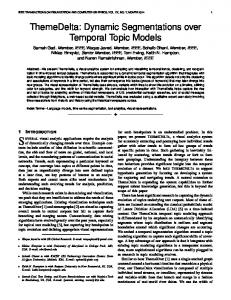
violations in the backtesting period Tbp and N0 = m − N1 . The test statistic tends to be small when N1 is “close” to the expected number of violations (PoF = 0 when πˆ = α ) and large when πˆ is either larger or smaller than α . Thus, the PoF testing procedure allows to reject both a too conservative VaR model (too large VaR estimates) and a poor VaR model (too small VaR estimates). The PoF test statistic, for m 7→ ∞, is distributed as a χ 2 random variable with 1 degree of freedom. If the test statistic is smaller than the γ -quantile of the χ12 distribution, where 1 − γ is the size of the test, the VaR model under examination is accepted and therefore can be considered reliable and effective. The test was computed at sizes 1 − γ = 10% and 1 − γ = 5%. This choice is motivated by the tradeoff between a small size and its costs in terms of Type II error: the smaller the size, the larger the probability of correctly choosing the null hypothesis but also the chance of a Type II error. In other words, setting a high probability (for example, 99%) of correctly choosing an effective VaR model, we also increase the probability of erroneously selecting an inappropriate VaR model, i.e. a VaR model with too many or too few violations. This can be seen from Fig. 1, which represents the PoF test statistic with m = 1, 320 (approximately five years of daily observations) and a 99% coverage level. The thick black curve represents the values of the test statistic as a function of the number of violations (x-axis), while the vertical dashed line is the expected number of violations. The horizontal lines represent three different critical values for the test, i.e. the γ -quantiles of the χ12 distribution with γ = 90, 95 and 99%. With a 1% size, the acceptance region of the test, represented by the lowermost thick grey line and including the numbers of violations such that the curve lies under the dashed horizontal line, is significantly larger than in the cases corresponding to the 5 and 10% levels, causing a Type II error that we deem too large. Figure 1: The PoF test statistic as a function of the number of VaR violations (at 99% coverage level) and the acceptance region as a function of the critical values corresponding to the 1, 5 and 10% sizes. PoF uncond. test statistic 99% Chi^2 (1) quantile: 6.63

10

95% Chi^2 (1) quantile: 3.84 90% Chi^2 (1) quantile: 2.71

6 4 2 0

POF statistic value

8

Exp.violations (1,320 obs.): 13

0

5

10

15

N° of VaR violations

16

20

25

5 Results Since the end of the second quarter 2007, equity markets became increasingly volatile due to the emerging financial crisis culminated, in September 2008, in the default of Lehman Brothers and continued until the end of 2008. In this period, the markets were characterized by unusually high volatility levels and huge losses due to deleveraging and flight to quality. The equity indexes of most industrialized countries wiped off almost all the capitalization accumulated since mid 2004 and, in some cases, even more. Similarly, the first quarter 2009 was dominated by high volatility and large losses worldwide. The models are implemented with three VaR probability levels (α ) equal to 5, 1 and 0.5%, thus assuming three coverage levels (95, 99 and 99.5%). The comparison of the overall performance of the models during the backtesting period takes into consideration the number of rejections of the null hypothesis for each VaR model: we count how many times each VaR model applied to the 15 loss time series (see Sect. 4.1) is rejected by the PoF test. This approach is justified because a model never rejected by the PoF test is certainly preferable to a rejected (one or more times) model: thus, a VaR model with fewer rejections is considered more accurate. More specifically, we adopt two different rankings. The first one considers the number of joint rejections with respect to the 99 and 99.5% VaR, so that it focuses on the behavior of VaR estimates in the tail of the loss distribution. The alternative ranking counts the number of rejections at 95% and is used along with the first one to complete the empirical evidence concerning VaR accuracy.

5.1

Preliminary results

Due to space limitations, we cannot show here all the results. We limit ourselves to detail the most important outcomes of the analysis of filtered losses. We use both formal testing procedures and graphical representations to evaluate the statistical properties of volatility-filtered losses. As for the graphs, three equally-sized filtered losses sub-samples are used for each asset, starting respectively on July 6, 2002, June 15, 2004 and December 27, 2005. The main findings can be summarized as follows. * The Ljung-Box test with 20 lags applied to each filtered loss sample (Zˆ j and Zˆ ∗j ) and to each asset, does not produce, in almost all cases, any evidence of serial correlation. Two exceptions are the FORD and Luxottica GARCH/EWMA residuals for which, at the extremes of the backtesting period, the test accepts the presence of autocorrelation. * The Q-Q plot of the filtered losses (with both EWMA and GARCH filters) with respect to the standard normal distribution shows the presence of heavy tails, in particular on the right tail (losses). This is more evident for the first and the third EWMA/GARCH filtered loss sub-sample. * The mean excess estimator plot used for choosing the threshold of the filtered losses sub-samples gives ambiguous results. In general, for most assets and sample periods, the expected linear pattern starts approximately at the threshold. In some cases, however, it is hard to identify a linear trend due to a large dispersion. In other cases, the linear trend seems to start above the threshold suggesting that the threshold should be larger.

17

5.2

Estimation results

The first issue of interest is the difference between the various estimates zˆq of the quantiles of the residuals obtained with the models under consideration. For Citigroup, Fig. 2(a) shows the estimates zˆq for the QMLE-GARCH POT model and the quantiles of the standard normal, all with a 99% coverage level. Similarly, Fig. 2(b) and (c) display zˆq for the remaining two POT models (t-GARCH and EWMA) and the estimated quantiles for dynamic models with the standardized Student-t distribution. The results for the other assets are similar and therefore not reported here. Figure 2: Citigroup. Estimates of the quantiles of the filtered losses zq with q =99 and 99.5%. Dynamic POT procedures.

03/05

03/06

03/07

03/08

03/09

t(v) EWMA 99,5% t(v) EWMA 99%

3.0 2.0

2.5

3.0 2.0

2.5

3.0 2.5 2.0 03/04

99,5 % 99 %

3.5

t(v) GARCH 99,5% t(v) GARCH 99%

EWMA(75,0.94) POT quantiles

4.0

99,5 % 99 %

3.5

N(0,1) 99,5 % N(0,1) 99 %

3.5

4.0

99,5 % 99 %

Student−t GARCH(1,1) POT quantiles

4.0

QMLE GARCH(1,1) POT quantiles

03/04

03/05

03/06

03/07

03/08

03/09

03/04

03/05

03/06

03/07

03/08

03/09

As can be seen from Fig. 2(a), the normal quantiles are significantly lower than the POT (GARCHQMLE, t-GARCH, EWMA) for the smallest VaR probabilities (1% and 0.5%). Thus, the assumption of a normal-driven dynamic VaR model leads to a larger risk of VaR underestimation, in particular at high coverage levels. This result is in line with the majority of VaR backtesting analyses in the literature (Angelidis et al., 2004; McNeil, Frey, 2000; Hung, et al. 2008). In figures 2(b) and (c) the POT t-GARCH and POT EWMA filtered losses quantiles are plotted against the standardized Student-t quantile obtained from the estimation of dynamic VaR models. The POT t-GARCH quantiles (Fig. 2(b)) are larger than the Student-t quantiles. In the last year of analysis, the POT t-GARCH quantiles declines slightly, whereas the t quantiles rise sharply; however, this feature is specific to Citigroup. The most interesting results can be seen by looking at Fig. 2(c): the POT quantiles estimated from EWMA filtered losses are significantly larger than the standardized Student-t quantiles. A second issue of interest is the relationship between the method used for volatility estimation and the estimated quantiles of the filtered losses. In this case the main messages of the empirical analysis are as follows. • For most assets and models, towards the end of Tbp (from August 2007, say), the numerical values 18

of the estimated quantiles increase significantly. • The EWMA estimated quantiles are generally larger than all other filtered losses estimated quantiles. This is probably due to both the weight structure of the EWMA filter with λ = 0.94 and the accuracy of the POT quantile estimator. With respect to a typical GARCH, the weight structure of the EWMA filter gives less weight to the very last observation but is more persistent: unusually high squared losses, frequently observed during the entire backtesting period, are not immediately overweighted, but the weight structure spreads its effects over a relatively long time horizon, contributing to constantly large and less volatile estimated quantiles with respect to the estimated quantiles of the GARCH residuals. • As a consequence of fewer excesses, the 99.5% estimated quantiles are more volatile than the 99% quantiles.

5.3

Backtesting results

Tables 4-10 in appendix A.1 show the full set of backtesting results for each asset involved in the analysis. The tables include two patterns: each horizontal box contains three rows with the results of the PoF test with three different VaR probabilities (5%, 1% and 0.5%). The first column shows the number of VaR violations, the second column the PoF test statistic, and the third the p-value associated with the numerical value of the PoF test statistic. For the 10 and 5% sizes, we evaluate the models with VaR probability levels α set to 5, 1 and 0.5% for all assets (see Sect. 4.1). It follows that, for either size of the test, the number of rejections for each model with a certain VaR probability α ranges from 0 to 15, namely the number of assets under consideration. 5.3.1 Results 1: test size 5% Table 2 summarizes the backtesting results when the size of the test is equal to 5%. The first column of Table 2 describes the VaR model tested, the central columns report the number of violations for each VaR probability and the last column shows the model ranking, as determined by the total number of rejections: the models are listed in ascending order, according to the total number of rejections at 99 and 99.5% coverage levels. Let us start with the worst performing VaR models, namely dynamic normal-driven VaR models. At 99 and 99.5%, for N(0,1)-GARCH, the number of rejections is 24 out of a maximum possible value of 30, while for the RiskMetricsTM VaR we get 28 rejections. Furthermore, as the VaR coverage level increases, the performance of both models gets worse. This is not surprising, given the well-known inadequacy of the normal distribution at high coverage levels in presence of fat tails in the filtered loss distributions. At 95%, the situation is quite different: the two dynamic normal-driven VaR models yield respectively 1 and 3 rejections and are at the top of the ranking. The two static VaR models (unconditional POT and unconditional HS) perform badly regardless of the VaR probability α : for all the three VaR probabilities, the number of PoF rejections ranges from 12 to

19

13, putting the two models at the bottom of the ranking (24 and 25 out of 30). This result is consistent with other backtesting studies (Bhattacharyya and Ritolia, 2008; McNeil and Frey, 2000) and is largely expected because of the inappropriateness of a static VaR model in a highly volatile period. A notable exception are the backtesting results of currencies, for which the two models perform well in 2 cases out of 3 (ZAR Rand and BRA Real). Fat-tailed dynamic VaR models (GARCH and EWMA models with Student-t and GED stochastic component) do not yield unequivocal performances. Looking at the total number of rejections with 1 and 0.5% VaR probabilities, the worst models are the EWMA fat-tailed specifications, both with 11 rejections out of 30. Furthermore, considering separately each VaR ranking, as the coverage level increases, the EWMA GED model performs progressively worse (3, 4 and 7 rejections out of 15), while the EWMA Student-t improves its performance (9, 7 and 4 rejections). However, at 95% VaR coverage, the EWMA GED model is in the top 5 of the ranking. The GARCH fat-tailed dynamic models achieve globally better results than the EWMA models, with 4 (GARCH Student-t) and 6 (GARCH GED) rejections out of 30; moreover, the GARCH t model is among the top 5 of the total rejection ranking. As in the previous case, the GARCH GED model worsens as the coverage level increases (1, 2 and 4 rejections), while the Student-t model improves (4, 2 and 2 rejections). Summarizing, GARCH fat-tailed models perform slightly better than EWMA models, but the use of a GED stochastic component seems to produce worse results as the coverage level gets larger. In general, DHS models work better at large VaR coverage levels than at low levels. The performance of the GED-GARCH and the N(0,1)-GARCH DHS models is identical at 5 and 1% VaR probability (4 and 3 rejections), but the GED model is preferable at 0.5%, with only one rejection. However, looking at the total number of rejections, these two DHS models perform similarly to fat-tailed dynamic models (4 and 6 rejections out of 30), which is acceptable but put the models out of the top 5 of the ranking. Consistently with the total rejection ranking, the best DHS models are the EWMA DHS and the tGARCH DHS model, respectively with 0 and 2 rejections out of 30. In particular, despite its simplicity and questionable non-parametric methodology, the EWMA DHS model is at the top of the ranking. The t-GARCH DHS is sometimes rejected (3 times out of 15) at 5% coverage, but is the third best model at 1 and 0.5% (1 rejection). One of the most interesting results is related to the POT models. At the top of Table 2 are listed the best VaR models according to the PoF test. On the basis of the overall ranking, dynamic POT models are the best-performing VaR approaches: the EMWA POT and the t-GARCH POT model are never rejected. The QMLE-GARCH POT models also perform well, with just 1 rejection out of 30: this result is in line with the outcomes obtained by McNeil and Frey (2000), Fernandez (2003), and Battacharya and Ritolia (2008). At 95% VaR coverage, both the QMLE and the t-GARCH POT models do not perform as well as at larger coverage levels, yielding respectively 3 and 4 rejections out of 15. Finally, the two GARCH POT VaR models turn out to be similar to the other dynamic fat-tailed VaR models. Figures 3 (DAX30 Index) – 6 (ZAR Rand in ¤) in appendix A.2 show the hit sequences with a 99% coverage level: each symbol on the graph represents a VaR violation, while the grey line shows the loss time series. As can be seen by looking at the top of each figure, violations originated by the two static 20

Table 2: Proportion of failures (POF) unconditional test. Confidence level: 95%. This table summarizes, for all assets analyzed (equities, indexes and currencies) and for each VaR model applied, the total number of rejection of the null hypothesis for correct VaR coverage using the POF unconditional coverage test (a.s. Chi squared) test with a confidence probability level of 95%

N◦ rejections

N◦ rejections

N◦ rejections

Total reject.

VaR 5%

VaR 1%

VaR 0,5%

(1%, 0.5%)

(max. 15)

(max. 15)

(max. 15)

(max. 30)

EWMA(75,0.94) POT

0

0

0

0

EWMA(75,0.94) DHS

0

0

0

0

t–GARCH(1,1) POT

4

0

0

0

QMLE–GARCH(1,1) POT

3

1

0

1

t–GARCH(1,1) DHS

3

1

1

2

t–GARCH(1,1) Student t

4

2

2

4

GED–GARCH(1,1) DHS

4

3

1

4

GED–GARCH(1,1) GED

1

2

4

6

N(0,1)–GARCH(1,1) DHS

4

3

3

6

EWMA(75,0.94) GED

3

4

7

11

EWMA(75,0.94) Student t

9

7

4

11

N(0,1)–GARCH(1,1) N(0,1)

1

11

13

24

Unconditional POT

12

12

12

24

Unconditional HS

12

13

12

25

3

13

15

28

VaR model

EWMA(75,0.94) N(0,1)

models are concentrated in the last 18 months, when equity markets have become very volatile. Even the two normal-driven dynamic models perform poorly during the financial crisis. Conversely, the EWMA DHS and EWMA POT models are associated to violations spread over the entire backtesting period. Differently from most of the models tested, these two VaR models are reliable both in quiet and extreme market conditions. This is an important feature: in case of highly volatile market conditions, they react more timely and provide better VaR estimates, minimizing the slippage of VaR-based capital charges over time. 5.3.2 Results 2: test size 10% Table 3 shows the results of the backtesting analysis when the size of the test is equal to 10%. Again, the worst VaR models according to the global ranking are the two normal-driven dynamic models (28 and 29 rejections) and the static VaR models. The first two result worse than in the previous ranking, falling in the last two positions of the global ranking. At 5% VaR probability, the performance of the two normal dynamic models deteriorates as well: in particular, the RiskMetricsTM model is rejected 8 times out of 15 with respect to 3 rejections at the 5% size. On the other hand, the GARCH-QMLE N(0,1) is significantly better at 5% VaR probability, with only 3 rejections out of 15. 21

Dynamic fat-tailed VaR models perform similarly to the preceding section: results are slightly less satisfactory for EWMA-filtered models than for GARCH models and, as the coverage levels increase, GED VaR models (both EWMA and GARCH) are rejected more often than Student-t based models. The only exception to the global failure of fat-tailed dynamic models is the Student-t GARCH model, whose performance is similar to the 5% size case (fourth out of 15 models). According to the total rejection-based ranking, dynamic historical models perform not very differently from the previous section. However, the Student-t DHS model now drops in the middle of the global ranking (6 rejections out of 30). The POT-based dynamic model is again at the top of the ranking. The first place is taken by the EWMA POT model with zero rejections out of 30, the second place by the Student-t POT model with 1 rejection and the third by the GARCH QMLE POT (3 rejections). At 5% VaR probability, the EWMA POT model is rejected 2 times out of 15, but this was the second smallest number of rejections of all models. Finally, the Student-t GARCH is not as efficient as the other POT models at 5% VaR probability, yielding 5 rejections out of 15. POT models are not the only well-performing approaches: the EWMA DHS model also reaches the top of both rankings (overall and at 5%), contrary to other DHS models, which turn out to be sufficiently accurate, but not at the top of the ranking. The EWMA DHS model is rejected twice and results the second best model at 5% probability level, while on the basis of the total rejection ranking it is rejected just once, similarly to the Student-t POT model. These outcomes put it at the second place of the ranking. Finally, the POT dynamic-based models are the most effective VaR estimation techniques, according to the total rejection ranking, also at the largest size employed. Only at 5% VaR probability the POT EWMA is sometimes rejected, but much more rarely than most of the other models. The other two POTbased models tested in our analysis achieve quite satisfactory results, even though the QMLE POT model is the worst POT model at both sizes. In conclusion, the main outcomes of the backtesting analysis are the following. * According to the PoF test at both 5 and 10% size, the POT EWMA and EWMA DHS models are the most reliable and effective ones when the VaR coverage level is 99 or 99.5%. At 95% coverage they are rejected in single cases, but are still preferable to all other models. * Dynamic fat-tailed models do not perform particularly well at the largest coverage level, lying mostly in the middle of the two rejection-based rankings. Only the t-GARCH approach has a performance comparable to the top-ranked models. * EWMA fat-tailed models are slightly less efficient than GARCH fat-tailed approaches. The number of rejections of the GED-based dynamic models (both EWMA and GARCH) gets larger as the VaR coverage level increases, contrary to the Student-t models. From the risk management perspective, the message is quite clear: the POT and DHS approaches with the EWMA volatility specification should be preferred, especially when tail risk is of paramount importance. 22

Table 3: Proportion of failures (PoF) test. Confidence level: 90%. This table summarizes, for all assets analyzed (equities, indexes and currencies) and for each VaR model applied, the total number of rejection of the null hypothesis for correct VaR coverage using the PoF unconditional coverage test (a.s. Chi squared) test with a confidence level of 90%

N◦ rejections

N◦ rejections

N◦ rejections

Total reject.

VaR 5%

VaR 1%

VaR 0,5%

(1%, 0.5%)

(max. 15)

(max. 15)

(max. 15)

(max. 30)

EWMA(75,0.94) POT

2

0

0

0

EWMA(75,0.94) DHS

2

1

0

1

t–GARCH(1,1) POT

5

0

1

1

QMLE–GARCH(1,1) POT

6

1

2

3

t–GARCH(1,1) Student t

5

2

2

4

t–GARCH(1,1) DHS

5

3

3

6

GED–GARCH(1,1) DHS

5

4

3

7

GED–GARCH(1,1) GED

1

4

4

8

EWMA(75,0.94) Student t

11

7

5

12

N(0,1)–GARCH(1,1) DHS

6

7

6

13

EWMA(75,0.94) GED

7

6

8

14

Unconditional HS

13

13

12

25

Unconditional POT

12

13

13

26

EWMA(75,0.94) N(0,1)

8

13

15

28

N(0,1)–GARCH(1,1) N(0,1)

3

15

14

29

VaR model

6 Conclusions This paper compares several dynamic VaR models commonly employed in market risk measurement. The time horizon includes the extreme market conditions observed during the financial crisis caused by the sub-prime mortgage crisis. The focus is primarily on the performance of a dynamic Peaks over Threshold procedure, which not only allows to take into account heavy-tailed risk factor distributions, but also has a strong theoretical justification. The results show that the POT model and the Dynamic Historical Simulation combined with the EWMA volatility specification are preferable, in particular at high VaR coverage levels. Whereas the good performance of the POT approach was not unexpected giving the features of the time series at hand and the sound theoretical foundations of the methodology, the success of DHS and EWMA is somewhat surprising in two respects. First, it is well-known that historical simulation does not perform particularly well in presence of extreme market movements. Second, the non-parametric EWMA estimator has weak theoretical justifications. A possible explanations for the first issue is that DHS, unlike standard historical simulation, uses a volatility filter, and this filter is likely to be the crucial tool for improving the performance of the method. As for the second one, the EWMA empirical performance is known to be rather good, and the weight structure captures reasonably well (better than typical GARCH models) 23

persistence effects and autocorrelation of squared losses. It should also be noted that EWMA works better than GARCH when associated to POT and DHS, but worse than GARCH when used in conjunction with ad hoc fat-tailed models. Several issues remain open for further investigations. First, we have only used “portfolios” consisting entirely of single assets, taking an index fund as a single asset. A generalization of the analysis to more realistic portfolios (for example, portfolios containing derivatives) does not appear straightforward but would be quite important. Second, it is well known that it is difficult to beat GARCH(1,1). In particular, moving either p or q to 2 does little to improve fit. On the other hand, FIGARCH models have recently been proposed as a tool for investigating long memory in squared returns. It would be of interest to check whether models of this family can provide better results than standard GARCH. Acknowledgements. We would like to thank Christopher L. Gilbert for a useful discussion and pointed remarks.

24

References [1] Angelidis T, Benos A and Degiannakis S (2004) The Use of GARCH Models in VaR Estimation. Statistical Methodology 1:105-128 [2] Baillie, RT and Bollerslev, T and Mikkelsen, HO (1996) Fractionally integrated generalized autoregressive conditional heteroskedasticity. J. of Econometrics 74:3-30 [3] Baixauli JS, Alvarez S (2006) Evaluating effects of excess kurtosis on VaR estimates: Evidence for international stock indices. R. of Quantitative Finance and Accounting 27:27-46 [4] Bank for International Settlements (2006) Amendment to the Capital Accord to incorporate market risks. Basel Committee on Banking Supervision [5] Bhattacharyya M, Ritolia G (2008) Conditional VaR using EVT - Towards a planned margin scheme. International Review of Financial Analysis 17:382-395 [6] Bollerslev T (1986) Generalized autoregressive conditional heteroskedasticity. J. of Econometrics 31:307-327 [7] Boudoukh J, Richardson M and Whitelaw R.F. (1998) The best of both worlds. Risk, 11: 64-67 [8] Christodoulou-Volos, C. and Siokis, F.M. (2006) Long range dependence in stock market returns. Applied Financial Economics, 16, 1331-1338. [9] Christoffersen PF (1998) Evaluating Interval Forecasts. International Economic Review 39:841-862 [10] Cont R (2001) Empirical properties of asset returns: stylized facts and statistical issues. Quantitative Finance 1:223-236 [11] Ding Z and Granger CWJ (1996) Modeling volatility persistence of speculative returns: A new approach. J. of Econometrics 73:185-1215 [12] Embrechts P, Klüppelberg C, Mikosch T (1997) Modelling Extremal Events for Insurance and Finance. Springer–Verlag, Berlin [13] Engle RF (1982) Autoregressive Conditional Heteroskedasticity with Estimates of the Variance of United Kingdom Inflation. Econometrica 50:987-1007 [14] Engle RF and Manganelli S (1999) CAViaR: Conditional Value at Risk by Quantile Regression. NBER, Working Paper 7341. [15] Fama EF (1965) The Behavior of Stock Market Prices. J. of Business 38:34-105 [16] Fernandez V (2003) Extreme Value Theory and Value at Risk. Revista de Analisis Economico – Economic Analysis Review 18:57-85

25

[17] Gil-Alana, L (2006) Fractional integration in daily stock market indexes. Review of Financial Economics 15, 28-48 [18] Kupiec P (1995) Techniques for Verifying the Accuracy of Risk Management Models. J. of Derivatives 3, 73-84 [19] Hung, JC, MC Lee and HC Liu (2008) Estimation of Value-at-Risk for energy commodities via fat-tailed GARCH models. Energy Economics, 30:1173-1191. [20] Mandelbrot B (1963) The Variations of Certain Speculative Prices. J. of Business, 36:394-419. [21] McNeil AJ and Frey R (2000) Estimation of tail-related risk measures for heteroscedastic financial time series: an extreme value approach. J. of Empirical Finance 7:271-300 [22] McNeil AJ, Frey R & Embrechts P, (2005) Quantitative Risk Management: Concepts, Techniques, and Tools Princeton University Press, Princeton and Oxford [23] McNeil AJ and Saladin T (1997) The Peaks over Threshold Method for Estimating High Quantiles of Loss Distributions. Proceedings of XXVIIth International ASTIN Colloquium 23-43, Cairns, Australia. [24] RiskMetrics, (1996) RiskMetricsTM – Technical Document. Fourth Edition, J.P. Morgan/Reuters, New York [25] R Development Core Team, (2009) R: A Language and Environment for Statistical Computing. R Foundation for Statistical Computing, Vienna, Austria [26] Würtz D et al. (2009) fExtremes: Rmetrics - Extreme Financial Market Data. R package version 290.76 [27] Würtz D, Chalabi Y and Miklovic M (2009) fGarch: Rmetrics - Autoregressive Conditional Heteroskedastic Modelling. R package version 2100.78

26

A A.1

Appendix Tables

Table 4: VaR backtesting – DAX30 (DAX) index and MIBTEL (MIB) index.VaR probabilities: 5%,1% and 0.5%.

VaR model

Violations

DAX LRtunc

QMLE–GARCH(1,1) POT

72 18 10

0,521 1,554 1,498

( 47,053 % ) ( 21,225 % ) ( 22,091 % )

87 19 7

6,524 2,293 0.026

( 1,065 % ) ( 13 % ) ( 87,251 % )

t–GARCH(1,1) POT

69 18 9

0,123 1,554 0,773

( 72,577 % ) ( 21,255 % ) ( 37,941 % )

87 19 8

6,524 2,293 0,286

( 1,065 % ) ( 13 % ) ( 59,287 % )

EWMA(75,0.94) POT

72 15 9

0,521 0,227 0,773

( 47,053 % ) ( 63,406 % ) ( 37,941 % )

76 14 9

1,572 0,052 0,798

( 20,986 % ) ( 82 % ) ( 37,163 % )

N(0,1)–GARCH(1,1) N(0,1)

74 24 20

0,933 7,120 17,602

( 33,398 % ) ( 0,762 % ) ( 0,003 % )

93 39 24

10,504 33,533 27,479

( 0,119 % ) (0%) (0%)

t–GARCH(1,1) Student t

78 21 9

2,099 3,9 0,773

( 14,735 % ) ( 4,829 % ) ( 37,941 % )

94 29 14

11,25 14,316 6,331

( 0,08 % ) ( 0,02 % ) ( 1,186 % )

GED–GARCH(1,1) GED

75 21 13

1,183 3,9 4,817

( 27,677 % ) ( 4,829 % ) ( 2,818 % )

92 27 14

9,782 11,254 6,331

( 0,176 % ) ( 0,08 % ) ( 1,186 % )

EWMA(75,0.94) N(0,1)

82 28 17

3,702 12,589 11,388

( 5,436 % ) ( 0,039 % ) ( 0,074 % )

88 38 27

7,127 31,349 35,686

( 0,759 % ) (0%) (0%)

EWMA(75,0.94) Student t

84 22 13

4,661 4,882 4,817

( 3,087 % ) ( 2,714 % ) ( 2,818 % )

94 29 16

11,25 14,316 9,647

( 0,08 % ) ( 0,015 % ) ( 0,19 % )

EWMA(75,0.94) GED

82 19 13

3,702 2,231 4,817

( 5,436 % ) ( 13,528 % ) ( 2,818 % )

88 29 16

7,127 14,316 9,647

( 0,759 % ) ( 0,015 % ) ( 0,19 % )

N(0,1)–GARCH(1,1) DHS

75 20 11

1,183 3,015 2,426

( 27,677 % ) ( 8,252 % ) ( 11,932 % )

84 18 12

4,862 1,605 3,595

( 2,745 % ) ( 20,51 % ) ( 5,795 % )

t–GARCH(1,1) DHS

76 19 10

1,461 2,231 1,498

( 22,684 % ) ( 13,528 % ) ( 22,091 % )

83 18 9

4,359 1,605 0,798

( 3,682 % ) ( 20,51 % ) ( 37,163 % )

GED–GARCH(1,1) DHS

75 19 11

1,183 2,231 2,426

( 27,677 % ) ( 13,528 % ) ( 11,932 % )

84 18 10

4,862 1,605 1,535

( 2,745 % ) ( 20,51 % ) ( 21,541 % )

EWMA(75,0.94) DHS

73 18 9

0,713 1,554 0,773

( 39,861 % ) ( 21,255 % ) ( 37,941 % )

76 17 9

1,572 1,031 0,798

( 20,986 % ) ( 31 % ) ( 37,163 % )

Unconditional POT

78 28 14

2,099 12,589 6,252

( 14,735 % ) ( 0,039 % ) ( 1,241 % )

103 30 17

18,968 15,954 11,499

( 0,001 % ) ( 0,01 % ) ( 0,07 % )

Unconditional HS

81 29 11

3,261 14,145 2,426

( 7,093 % ) ( 0,017 % ) ( 11,932 % )

105 30 17

20,92 15,954 11,499

(0%) ( 0,01 % ) ( 0,07 % )

p–value

Violations

MIB LRtunc

p–value

Backtesting length: 1320. POT excesses: 104. Sample length: 800. Expected VaR violations: 66 (5%), 13 (1%), 7 (0,5%). Backtesting length: 1317; POT excesses: 108; Samples size: 825. Expected VaR violations: 66 (5%), 13 (1%), 7 (0,5%).

27

Table 5: VaR backtesting – NIKKEI 225 index (N225) and Credit Suisse Group (CS) (NYSE). VaR probabilities: 5%,1% and 0.5%. N225

CS

VaR model

Violations

LRtunc

p–value

Violations

LRtunc

p–value

QMLE–GARCH(1,1) POT

70 14 8

0,647 0,124 0,391

(42,125 % ) (72,477 % ) (53,222 % )

74 15 10

1,144 0,272 1,582

(28,481 % ) (60,211 % ) (20,845 % )

t–GARCH(1,1) POT

69 16 8

0,461 0,785 0,391

( 49,702 % ) ( 37,575 % ) ( 53,222 % )

71 16 10

0,492 0,615 1,582

( 48,319 % ) ( 43,301 % ) ( 20,845 % )

EWMA(75,0.94) POT

67 16 8

0,183 0,785 0,391

( 66,916 % ) ( 37,575 % ) ( 53,222 % )

59 15 8

0,681 0,272 0,306

( 40,935 % ) ( 60,211 % ) ( 58,033 % )

N(0,1)–GARCH(1,1) N(0,1)

75 21 15

2,02 4,538 8,506

( 15,522 % ) ( 3,315 % ) ( 0,354 % )

56 23 16

1,492 6,199 9,778

( 22,193 % ) ( 1,278 % ) ( 0,177 % )

t–GARCH(1,1) Student–t

75 17 10

2,02 1,309 1,776

( 15,522 % ) ( 25,257 % ) ( 18,266 % )

63 14 10

0,094 0,064 1,582

( 75,941 % ) ( 80,044 % ) ( 20,845 % )

GED–GARCH(1,1) GED

73 17 13

1,383 1,309 5,332

( 23,955 % ) ( 25,257 % ) ( 2,093 % )

58 14 11

0,915 0,064 2,534

( 33,885 % ) ( 80,044 % ) ( 11,139 % )

EWMA(75,0.94) N(0,1)

77 25 19

2,771 9,326 16,414

( 9,602 % ) ( 0,226 % ) ( 0,005 % )

55 21 17

1,836 4,093 11,644

( 17,542 % ) ( 4,306 % ) ( 0,064 % )

EWMA(75,0.94) Student–t

80 21 14

4,102 4,538 6,847

( 4,282 % ) ( 3,315 % ) ( 0,888 % )

60 17 11

0,482 1,084 2,534

( 48,747 % ) ( 29,775 % ) ( 11,139 % )

EWMA(75,0.94) GED

76 20 15

2,381 3,573 8,506

( 12,279 % ) ( 5,873 % ) ( 0,354 % )

55 17 13

1,836 1,084 4,974

( 17,542 % ) ( 29,775 % ) ( 2,572 % )

N(0,1)–GARCH(1,1) DHS

73 15 11

1,383 0,387 2,783

( 23,955 % ) ( 53,401 % ) ( 9,528 % )

78 19 8

2,413 2,375 0,306

( 12,031 % ) ( 12,332 % ) ( 58,033 % )

t–GARCH(1,1) DHS

72 17 11

1,108 1,309 2,783

( 29,247 % ) ( 25,257 %) ( 9,528 % )

78 20 8

2,413 3,183 0,306

( 12,031 % ) ( 7,441 % ) ( 58,033 % )

GED–GARCH(1,1) DHS

72 17 11

1,108 1,309 2,783

( 29,247 % ) ( 25,257 %) ( 9,528 % )

75 20 8

1,419 3,183 0,306

( 23,353 % ) ( 7,441 % ) ( 58,033 % )

EWMA(75,0.94) DHS

70 17 8

0,647 1,309 0,391

( 42,125 % ) ( 25,257 %) ( 53,222 % )

68 17 8

0,107 1,084 0,306

( 74,305 % ) ( 29,775 % ) ( 58,033 % )

Unconditional POT

84 27 16

6,251 12,223 10,3

( 1,242 % ) ( 0,047 % ) ( 0,133 % )

110 34 24

26,811 23,459 27,721

(0%) (0%) (0%)

Unconditional HS

86 27 17

7,479 12,223 12,221

( 0,624 % ) ( 0,047 % ) ( 0,047 % )

113 36 22

30,239 27,463 22,641

(0%) (0%) (0%)

Backtesting length: 1273; POT excesses: 101; Samples size: 776. Expected VaR violations 64 (5%), 13 (1%), 6 (0,5%). Backtesting length: 1308; POT excesses: 103; sample size: 791. Expected VaR violations: 65 (5%), 13 (1%), 6 (0,5%).

28

Table 6: VaR backtesting – Italcementi S.p.a. (IT) and Luxottica S.p.a. (LUX). VaR probabilities: 5%,1% and 0.5%. IT

LUX

VaR model

Violations

LRtunc

p–value

Violations

LRtunc

p–value

QMLE–GARCH(1,1) POT

82 17 10

3,752 1,001 1,509

( 5,273 % ) ( 31,699 % ) ( 21,933 % )

78 15 7

2,137 0,232 0,023

( 14,375 % ) ( 63,004 % ) ( 88,027 % )

t–GARCH(1,1) POT

81 18 10

3,309 1,569 1,509

( 6,891 % ) ( 21,042 % ) ( 21,933 % )

72 16 7

0,539 0,553 0,023

( 46,269 % ) ( 45,695 % ) ( 88,027 % )

EWMA(75,0.94) POT

73 15 10

0,734 0,232 1,509

( 39,145 % ) ( 63,004 % ) ( 21,933 % )

69 9 5

0,132 1,532 0,431

( 71,625 % ) ( 21,574 % ) ( 51,174 % )

N(0,1)–GARCH(1,1) N(0,1)

80 22 16

2,892 4,909 9,575

( 8,904 % ) ( 2,672 % ) ( 0,197 % )

63 20 10

0,155 3,035 1,509

( 69,347 % ) ( 8,147 % ) ( 21,993 % )

t–GARCH(1,1) Student–t

83 18 9

4,222 1,569 0,78

( 3,99 % ) ( 21,042 % ) ( 37,718 % )

67 9 5

0,013 1,532 0,431

( 90,977 % ) ( 21,574 % ) ( 51,174 % )

GED–GARCH(1,1) GED

79 16 9

2,501 0,553 0,78

( 11,377 % ) ( 45,695 % ) ( 37,718 % )

60 10 6

0,611 0,865 0,058

( 43,453 % ) ( 35,234 % ) ( 80,905 % )

EWMA(75,0.94) N(0,1)

82 18 16

3,752 1,569 9,575

( 5,273 % ) ( 21,042 % ) ( 0,197 % )

66 21 13

0,001 3,924 4,837

( 98,993 % ) ( 4,761 % ) ( 2,786 % )

EWMA(75,0.94) Student–t

91 16 8

8,881 0,553 0,275

( 0,288 % ) ( 45,695 % ) ( 59,987 % )

77 13 5

1,801 0,004 0,431

( 17,961 % ) ( 95,138 % ) ( 51,174 % )

EWMA(75,0.94) GED(υ )

81 15 8

3,309 0,232 0,275

( 6,891 % ) ( 63,004 % ) ( 59,987 % )

65 12 5

0,019 0,117 0,431

( 88,931 % ) ( 73,192 % ) ( 51,174 % )

N(0,1)–GARCH(1,1) DHS

77 20 10

1,801 3,035 1,509

( 17,96 % ) ( 8,147 % ) ( 21,933 % )

81 18 10

3,309 1,569 1,509

( 6,891 % ) ( 21,042 % ) ( 21,933 % )

t–GARCH(1,1) DHS

79 19 11

2,501 2,248 2,44

( 11,377 % ) ( 13,375 % ) ( 11,831 % )

77 19 9

1,801 2,248 0,781

( 17,961 % ) ( 13,375 % ) ( 37,718 % )

GED–GARCH(1,1) DHS

79 18 11

2,501 1,569 2,44

( 11,377 % ) ( 21,042 % ) ( 11,831 % )

77 19 10

1,801 2,248 1,509

( 17,961 % ) ( 13,375 % ) ( 21,993 % )

EWMA(75,0.94) DHS

68 15 10

0,057 0,232 1,509

( 81,134 % ) ( 63,004 % ) ( 21,933 % )

68 13 7

0,057 0,004 0,023

( 81,134 % ) ( 95,138 % ) ( 88,027 % )

Unconditional POT

105 33 20

20,604 21,116 17,643

( 0,001 % ) (0%) ( 0,003 % )

98 23 13

14,202 5,986 4,837

( 0,016 % ) ( 1,442 % ) ( 2,786 % )

Unconditional HS

108 33 21

23,662 21,116 19,927

(0%) (0%) ( 0,001 % )

102 28 16

17,732 12,634 9,575

( 0,003 % ) ( 0,038 % ) ( 0,197 % )

Backtesting length: 1322; POT excesses: 108, Samples size: 825. Expected VaR violations: 66 (5%), 13 (1%), 7 (0,5%). Backtesting length: 1322; POT excesses: 108, Samples size: 825. Expected violations: 66 (5%), 13 (1%), 7 (0,5%).

29

Table 7: VaR backtesting – Citigroup Inc. (C) and Vodafone Plc (VOD) VaR probabilities: 5%,1% and 0.5%. C

VOD

VaR model

Violations

LRtunc

p–value

Violations

LRtunc

p–value

QMLE–GARCH(1,1) POT

80 21 12

3,213 4,093 3,672

( 7,306 % ) ( 4,306 % ) ( 5,539 % )

85 15 7

5,673 0,272 0,032

( 1,723 % ) ( 60,211 % ) ( 85,851 % )

t–GARCH(1,1) POT

86 18 10

6,241 1,673 1,582

( 1,248 % ) ( 19,585 % ) ( 20,845 % )

83 16 7

4,611 0,615 0,032

( 3,176 % ) ( 43,301 % ) ( 85,851 % )

EWMA(75,0.94) POT

81 15 8

3,653 0,272 0,306

( 5,597 % ) ( 60,211 % ) ( 58,033 % )

77 12 7

2,054 0,093 0,032

( 15,178 % ) ( 76,085 % ) ( 85,851 % )

N(0,1)–GARCH(1,1) N(0,1)

74 32 21

1,144 19,695 20,328

( 28,481 % ) ( 0,001 % ) ( 0,001 % )

71 22 15

0,492 5,101 8,039

( 48,319 % ) ( 2,393 % ) ( 0,458 % )

t–GARCH(1,1) Student–t

80 18 13

3,213 1,673 4,974

( 7,306 % ) ( 19,585 % ) ( 2,572 % )

71 16 8

0,492 0,615 0,306

( 48,319 % ) ( 43,301 % ) ( 58,033 % )

GED–GARCH(1,1) GED

72 20 14

0,681 3,183 6,434

( 40,964 % ) ( 7,441 % ) ( 1,119 % )

69 15 9

0,205 0,272 0,832

( 65,066 % ) ( 60,211 % ) ( 36,174 % )

EWMA(75,0.94) N(0,1)

78 26 19

2,413 10,014 15,727

( 12,031 % ) ( 0,155 % ) ( 0,007 % )

68 19 13

0,107 2,375 4,974

( 74,305 % ) ( 12,332 % ) ( 2,572 % )

EWMA(75,0.94) Student–t

93 21 11

10,904 4,093 2,534

( 0,096 % ) ( 4,306 % ) ( 11,139 % )

79 14 7

2,8 0,064 0,032

( 9,429 % ) ( 80,041 % ) ( 85,851 % )

EWMA(75,0.94) GED

78 21 12

2,413 4,093 3,671

( 12,031 % ) ( 4,306 % ) ( 5,539 % )

67 13 7

0,041 0 0,032

( 83,975 % ) ( 98,225 % ) ( 85,851 % )

N(0,1)–GARCH(1,1) DHS

80 21 13

3,213 4,093 4,974

( 7,306 % ) ( 4,306 % ) ( 2,572 % )

85 20 11

5,673 3,183 2,534

( 1,723 % ) ( 7,441 % ) ( 11,139 % )

t–GARCH(1,1) DHS

85 19 13

5,673 2,375 4,974

( 1,723 % ) ( 12,332 % ) ( 2,572 % )

81 20 11

3,653 3,183 2,534

( 5,597 % ) ( 7,441 % ) ( 11,139 % )

GED–GARCH(1,1) DHS

83 19 14

4,611 2,375 6,434

( 3,176 % ) ( 12,332 % ) ( 1,119 % )

86 21 11

6,241 4,093 2,534

( 1,248 % ) ( 4,306 % ) ( 11,139 % )

EWMA(75,0.94) DHS

81 20 10

3,653 3,183 1,582

( 5,597 % ) ( 7,441 % ) ( 20,845 % )

74 15 7

1,144 0,272 0,032

( 28,481 % ) ( 60,211 % ) ( 85,851 % )

Unconditional POT

142 60 34

71,809 90,672 57,756

(0%) (0%) (0%)

96 20 13

13,254 3,183 4,974

( 0,027 % ) ( 7,441 % ) ( 2,572 % )

Unconditional HS

146 56 35

78,646 78,477 61,126

(0%) (0%) (0%)

94 26 13

11,665 10,014 4,974

( 0,064 % ) ( 0,155 % ) ( 2,572 % )

Backtesting length: 1308; POT excesses: 103; Sample size: 792; Expected VaR violations: 65 (5%), 13 (1%), 6 (0,5%). Backtesting length: 1308; POT excesses: 103; Samples size: 792. Expected VaR violations: 65 (5%), 13 (1%), 6 (0,5%).

30

Table 8: VaR backtesting – Ford Motor Company (F) and General Motors (GM). VaR probabilities: 5%,1% and 0.5%.

F

GM

VaR model

Violations

LRtunc

p–value

Violations

LRtunc

p–value

QMLE–GARCH(1,1) POT

67 18 12

0,041 1,673 3,671

( 83,975 % ) ( 19,585 % ) ( 5,539 % )

84 16 8

5,129 0,615 0,306

( 2,353 % ) ( 43,301 % ) ( 58,033 % )

t–GARCH(1,1) POT

72 18 12

0,681 1,673 3,671

( 40,964 % ) ( 19,585 % ) ( 5,539 % )

84 13 8

5,129 0,01 0,306

( 2,353 % ) ( 98,225 % ) ( 58,033 % )

EWMA(75,0.94) POT

67 13 10

0,041 0,001 1,582

( 83,975 % ) ( 98,225 % ) ( 20,845 % )

81 13 6

3,653 0,01 0,046

( 5,597 % ) ( 98,225 % ) ( 83,001 % )

N(0,1)–GARCH(1,1) N(0,1)

57 20 17

1,185 3,183 11,644

( 27,635 % ) ( 7,441 % ) ( 0,064 % )

75 28 18

1,419 12,995 13,629

( 23,353 % ) ( 0,032 % ) ( 0,022 % )

t–GARCH(1,1) Student–t

69 17 9

0,205 1,084 0,832

( 65,066 % ) ( 29,775 % ) ( 36,174 % )

83 12 7

4,611 0,093 0,032

( 3,176 % ) ( 76,085 % ) ( 85,851 % )

GED–GARCH(1,1) GED

60 18 11

0,482 1,673 2,534

( 48,747 % ) ( 19,585 % ) ( 11,139 % )

76 15 9

1,723 0,272 0,832

( 18,934 % ) ( 60,211 % ) ( 36,174 % )

EWMA(75,0.94) N(0,1)

72 29 16

0,681 14,537 9,778

( 40,964 % ) ( 0,014 % ) ( 0,177 % )

81 29 24

3,653 14,537 27,721

( 5,597 % ) ( 0,014 % ) (0%)

EWMA(75,0.94) Student–t

78 15 11

2,413 0,272 2,534

( 12,031 % ) ( 60,211 % ) ( 11,139 % )

91 22 8

9,425 5,1 0,306

( 0,211 % ) ( 2,393 % ) ( 58,033 % )

EWMA(75,0.94) GED

72 16 13

0,681 0,615 4,974

( 40,964 % ) ( 43,301 % ) ( 2,572 % )

80 20 8

3,213 3,183 0,306

( 7,306 % ) ( 7,441 % ) ( 58,033 % )

N(0,1)–GARCH(1,1) DHS

67 20 12

0,041 3,183 3,671

( 83,975 % ) ( 7,441 % ) ( 5,539 % )

84 26 14

5,129 10,014 6,434

( 2,353 % ) ( 0,155 % ) ( 1,119 % )

t–GARCH(1,1) DHS

73 19 12

0,897 2,375 3,671

( 34,348 % ) ( 12,332 % ) ( 5,539 % )

83 21 9

4,611 4,093 0,832

( 3,176 % ) ( 4,306 % ) ( 36,174 % )

GED–GARCH(1,1) DHS

72 19 12

0,681 2,375 3,671

( 40,964 % ) ( 12,332 % ) ( 5,539 % )

84 23 10

5,129 6,199 1,582

( 2,353 % ) ( 1,278 % ) ( 20,845 % )

EWMA(75,0.94) DHS

68 19 10

0,107 2,375 1,582

( 74,305 % ) ( 12,332 % ) ( 20,845 % )

80 15 9

3,213 0,272 0,832

( 7,306 % ) ( 60,211 % ) ( 36,174 % )

Unconditional POT

100 26 14

16,702 10,014 6,434

( 0,004 % ) ( 0,155 % ) ( 1,119 % )

130 38 19

52,841 31,697 15,727

(0%) (0%) ( 0,007 % )

Unconditional HS

102 33 17

18,557 21,546 11,644

( 0,002 % ) (0%) ( 0,064 % )

132 44 23

55,837 45,658 25,137

(0%) (0%) (0%)

Backtesting length: 1308; POT excesses: 103; Samples size: 792 Expected violations: 65 (5%), 13 (1%), 6 (0,5%). Backtesting length: 1308; POT excesses: 103; Samples size: 792. Expected violations: 65 (5%), 13 (1%), 6 (0,5%).

31

Table 9: VaR backtesting – Microsoft Corp. (MSFT) and Unicredit Group (UCG). VaR probabilities: 5%,1% and 0.5%.

MSFT

UCG

VaR model

Violations

LRtunc

p–value

Violations

LRtunc

p–value

QMLE–GARCH(1,1) POT

74 19 8

1,144 2,375 0,306

( 28,481 % ) ( 12,332 % ) ( 58,033 % )

81 12 6

2,984 0,145 0,072

( 8,407 % ) ( 70,356 % ) ( 78,838 % )

t–GARCH(1,1) POT

77 15 7

2,054 0,272 0,032

( 15,178 % ) ( 60,211 % ) ( 85,851 % )

79 11 5

2,221 0,448 0,465

( 13,612 % ) ( 50,325 % ) ( 49,515 % )

EWMA(75,0.94) POT

72 15 6

0,681 0,272 0,046

( 40,964 % ) ( 60,211 % ) ( 83,001 % )

80 13 5

2,591 0,010 0,465

( 10,757 % ) ( 92,079 % ) ( 49,515 % )

N(0,1)–GARCH(1,1) N(0,1)

67 22 17

0,041 5,1 11,644

( 83,975 % ) ( 2,393 % ) ( 0,064 % )

73 20 12

0,589 2,892 3,44

( 44,291 % ) ( 8,902 % ) ( 6,363 % )

t–GARCH(1,1) Student–t

61 14 6

0,318 0,064 0,046

( 57,254 % ) ( 80,044 % ) ( 83,001 % )

76 12 5

1,279 0,145 0,465

( 25,821% ) ( 70,356 % ) ( 49,515 % )

GED–GARCH(1,1) GED

58 12 8

0,915 0,093 0,306

( 33,885 % ) ( 76,085 % ) ( 58,033 % )

74 10 5

0,791 0,935 0,465

( 37,395 % ) ( 33,359 % ) ( 49,515 % )

EWMA(75,0.94) N(0,1)

51 21 14

3,599 4,093 6,434

( 5,781 % ) ( 4,306 % ) ( 1,119 % )

80 26 16

2,591 9,464 9,377

( 10,757 % ) ( 0,209 % ) ( 0,221 % )

EWMA(75,0.94) Student–t

69 14 8

0,205 0,064 0,306

( 65,066 % ) ( 80,044 % ) ( 58,033 % )

83 16 7

3,852 0,496 0,015

( 4,967 % ) ( 48,143 % ) ( 90,198 % )

EWMA(75,0.94) GED

52 14 11

3,099 0,064 2,534

( 7,834 % ) ( 80,044 % ) ( 11,139 % )

80 15 7

2,591 0,196 0,015

( 10,757 % ) ( 65,831 % ) ( 90,198 % )

N(0,1)–GARCH(1,1) DHS

98 26 13

14,934 10,014 4,974

( 0,011 % ) ( 0,155 % ) ( 2,572 % )

79 15 10

2,221 0,196 1,438

( 13,612 % ) ( 65,831 % ) ( 23,052 % )

t–GARCH(1,1) DHS

75 19 9

1,419 2,375 0,832

( 23,353 % ) ( 12,332 % ) ( 36,174 % )

81 13 9

2,984 0,010 0,731

( 8,407 % ) ( 92,079 % ) ( 39,289 % )

GED–GARCH(1,1) DHS

77 21 10

2,054 4,093 1,582

( 15,178 % ) ( 4,306 % ) ( 20,845 % )

81 13 10

2,984 0,010 1,438

( 8,407 % ) ( 92,079 % ) ( 23,052 % )

EWMA(75,0.94) DHS

71 18 8

0,492 1,673 0,306

( 48,319 % ) ( 19,585 % ) ( 58,033 % )

78 16 8

1,881 0,496 0,246

( 17,033 % ) ( 48,143 % ) ( 61,956 % )

Unconditional POT

103 28 12

19,516 12,955 3,671

( 0,001 % ) ( 0,032 % ) ( 5,539 % )

129 41 23

48,492 37,249 24,434

(0%) (0%) (0%)

Unconditional HS

103 33 17

19,516 21,546 11,644

( 0,001 % ) (0%) ( 0,064 % )

135 43 24

57,297 41,918 26,976

(0%) (0%) (0%)

Backtesting length: 1308; POT excesses: 103; Samples size: 792. Expected VaR violations: 65 (5%), 13 (1%), 6 (0,5%). Backtesting length: 1336; POT excesses: 108; Samples size: 825. Expected VaR violations: 67 (5%), 13 (1%), 7 (0,5%).

32

Table 10: VaR backtesting – GBP British Pound (in ¤) and ZAR South African Rand (in ¤). VaR probabilities: 5%,1% and 0.5%.

GBP

ZAR

VaR model

Violations

LRtunc

p–value

Violations

LRtunc

p–value

QMLE–GARCH(1,1) POT

70 13 7

0,196 0,006 0,019

( 65,768 % ) ( 93,605 % ) ( 89,114 % )

63 12 7

0,192 0,131 0,019

( 66,149 % ) ( 71,767 % ) ( 89,114 % )

t–GARCH(1,1) POT

74 12 7

0,872 0,131 0,019

( 35,032 % ) ( 71,767 % ) ( 89,114 % )

68 12 8

0,038 0,131 0,261

( 84,588 % ) ( 71,767 % ) ( 60,97 % )

EWMA(75,0.94) POT

78 11 6

2,006 0,423 0,065

( 15,664 % ) ( 51,524 % ) ( 79,868 % )

63 15 6

0,192 0,213 0,065

( 66,149 % ) ( 64,414 % ) ( 79,868 % )

N(0,1)–GARCH(1,1) N(0,1)

74 22 13

0,872 4,815 4,769

( 35,032 % ) ( 2,821 % ) ( 2,898 % )

80 24 19

2,738 7,037 15,328

( 9,797 % ) ( 0,798 % ) ( 0,009 % )

t–GARCH(1,1) Student–t

79 15 11

2,359 0,213 2,393

( 12,457 % ) ( 64,414 % ) ( 12,188 % )

86 18 11

5,563 1,518 2,393

( 1,835 % ) ( 21,795 % ) ( 12,188 % )

GED–GARCH(1,1) GED

74 16 11

0,872 0,524 2,393

( 35,032 % ) ( 46,912 % ) ( 12,188 % )

79 20 11

2,359 2,963 2,393

( 12,457 % ) ( 8,518 % ) ( 12,188 % )

EWMA(75,0.94) N(0,1)

84 27 15

4,519 11 7,768

( 3,353 % ) ( 0,091 % ) ( 0,532 % )

87 30 22

6,122 15,644 22,145

( 1,335 % ) ( 0,008 % ) (0%)

EWMA(75,0.94) Student–t

90 19 9

7,947 2,187 0,755

( 0,482 % ) ( 13,918 % ) ( 38,5 % )

96 24 15

12,234 7,037 7,768

( 0,047 % ) ( 0,798 % ) ( 0,532 % )

EWMA(75,0.94) GED

84 19 11

4,519 2,187 2,393

( 3,353 % ) ( 13,918 % ) ( 12,188 % )

87 24 15

6,122 7,037 7,768

( 1,335 % ) ( 0,798 % ) ( 0,532 % )

N(0,1)–GARCH(1,1) DHS

67 15 10

0,005 0,213 1,473

( 94,488 % ) ( 64,414 % ) ( 22,488 % )

67 13 10

0,005 0,006 1,473

( 94,488 % ) ( 93,605 % ) ( 22,488 % )

t–GARCH(1,1) DHS

69 16 10

0,102 0,524 1,473

( 74,971 % ) ( 46,912 % ) ( 22,488 % )

68 12 9

0,038 0,131 0,755

( 84,588 % ) ( 71,767 % ) ( 38,5 % )

GED–GARCH(1,1) DHS

67 15 10

0,005 0,213 1,473

( 94,488 % ) ( 64,414 % ) ( 22,488 % )

68 12 10

0,038 0,131 1,473

( 84,588 % ) ( 71,767 % ) ( 22,488 % )

EWMA(75,0.94) DHS

73 14 9

0,659 0,038 0,755

( 41,675 % ) ( 84,614 % ) ( 38,5 % )

67 15 9

0,005 0,213 0,755

( 94,488 % ) ( 64,414 % ) ( 38,5 % )

Unconditional POT

103 34 17

18,254 22,783 11,309

( 0,002 % ) (0%) ( 0,077 % )

70 14 9

0,196 0,038 0,755

( 32,751 % ) ( 84,614 % ) ( 38,5 % )

Unconditional HS

104 35 22

19,2 24,724 22,145

( 0,001 % ) (0%) (0%)

68 14 8

0,038 0,038 0,261

( 84,588 % ) ( 84,614 % ) ( 60,97 % )

Backtesting length: 1329; POT excesses: 105; Samples size: 806. Expected VaR violations: 66 (5%), 13 (1%), 7 (0,5%). Backtesting length: 1329; POT excesses: 105; Samples size: 806. Expected violations: 66 (5%), 13 (1%), 7 (0,5%).

33

A.2

Figures

Figure 3: DAX30 Index. VaR 99% backtesting from March, 2 2004 to May, 9 2009. Each symbol represents a VaR violation for the VaR models listed in the legend. Static POT: [ 28 ] 15

Static HS: [ 29 ] QMLE−GARCH(1,1) POT: [ 18 ] N(0,1)−GARCH(1,1) N(0,1): [ 24 ] N(0,1)−GARCH(1,1) DHS: [ 20 ] 10

EWMA(75,0.94) N(0,1): [ 28 ]

5

EWMA(75,0.94) DHS: [ 18 ]

−5

0

% Losses − % VaR

EWMA(75,0.94) POT: [ 15 ]

04/03

04/07

04/11

05/03

05/07

05/11

06/03

06/07

06/11

07/03

07/07

07/11

08/03

08/07

08/11

09/03

05/03

05/07

05/11

06/03

06/07

06/11

07/03

07/07

07/11

08/03

08/07

08/11

09/03

t−GARCH(1,1) POT: [ 18 ] 15

t−GARCH(1,1) Student−t: [ 21 ] t−GARCH(1,1) DHS: [ 19 ] GED−GARCH(1,1) GED: [ 21 ] GED−GARCH(1,1) DHS: [ 19 ] 10 5 0 −5

% Losses − % VaR

EWMA(75,0.94) Student−t: [ 22 ] EWMA(75,0.94) GED: [ 19 ]

04/03

04/07

04/11

34

25

Figure 4: Citigroup Corp. VaR 99% backtesting from March, 2 2004 to May, 9 2009. Each symbol represents a VaR violation for the VaR models listed in the legend. Static POT: [ 60 ] Static HS: [ 56 ] 20

QMLE−GARCH(1,1) POT: [ 21 ] N(0,1)−GARCH(1,1) N(0,1): [ 32 ] N(0,1)−GARCH(1,1) DHS: [ 21 ] EWMA(75,0.94) N(0,1): [ 26 ]

10

EWMA(75,0.94) DHS: [ 20 ]

−5

0

5

% Losses − % VaR

15

EWMA(75,0.94) POT: [ 15 ]

25

04/03

04/07

04/11

05/03

05/07

05/11

06/03

06/07

06/11

07/03

07/07

07/11

08/03

08/07

08/11

09/03

05/03

05/07

05/11

06/03

06/07

06/11

07/03

07/07

07/11

08/03

08/07

08/11

09/03

t−GARCH(1,1) POT: [ 18 ] t−GARCH(1,1) Student−t: [ 18 ]

20

t−GARCH(1,1) DHS: [ 19 ] GED−GARCH(1,1) GED: [ 20 ] GED−GARCH(1,1) DHS: [ 19 ]

10 5 0 −5

% Losses − % VaR

15

EWMA(75,0.94) Student−t: [ 21 ] EWMA(75,0.94) GED: [ 21 ]

04/03

04/07

04/11

35

Figure 5: Vodafone Plc. VaR 99% backtesting from March, 2 2004 to May, 9 2009. Each symbol represents a VaR violation for the VaR models listed in the legend.

15

Static POT: [ 20 ] Static HS: [ 26 ] QMLE−GARCH(1,1) POT: [ 15 ] N(0,1)−GARCH(1,1) N(0,1): [ 22 ]

10

N(0,1)−GARCH(1,1) DHS: [ 20 ] EWMA(75,0.94) POT: [ 12 ] EWMA(75,0.94) N(0,1): [ 19 ]

5 −5

0

% Losses

EWMA(75,0.94) DHS: [ 15 ]

04/03

04/07

04/11

05/03

05/07

05/11

06/03

06/07

06/11

07/03

07/07

07/11

08/03

08/07

08/11

09/03

05/03

05/07

05/11

06/03

06/07

06/11

07/03

07/07

07/11

08/03

08/07

08/11

09/03

15

t−GARCH(1,1) POT: [ 16 ] t−GARCH(1,1) Student−t: [ 16 ] t−GARCH(1,1) DHS: [ 20 ] GED−GARCH(1,1) GED: [ 15 ] EWMA(75,0.94) Student−t: [ 14 ]

0

5

EWMA(75,0.94) GED: [ 13 ]

−5

% Losses

10

GED−GARCH(1,1) DHS: [ 21 ]

04/03

04/07

04/11

36

Figure 6: ZAR Rand (in ¤). VaR 99% backtesting from March, 2 2004 to May, 9 2009. Each symbol represents a VaR violation for the VaR models listed in the legend. 15

Static POT: [ 14 ] Static HS: [ 14 ] QMLE−GARCH(1,1) POT: [ 12 ] N(0,1)−GARCH(1,1) N(0,1): [ 24 ] 10

N(0,1)−GARCH(1,1) DHS: [ 13 ] EWMA(75,0.94) POT: [ 15 ] EWMA(75,0.94) N(0,1): [ 30 ]

5 −5

0

% Losses

EWMA(75,0.94) DHS: [ 15 ]

04/03

04/07

04/11

05/03

05/07

05/11

06/03

06/07

06/11

07/03

07/07

07/11

08/03

08/07

08/11

09/03

05/03

05/07

05/11

06/03

06/07

06/11

07/03

07/07

07/11

08/03

08/07

08/11

09/03

15

t−GARCH(1,1) POT: [ 12 ] t−GARCH(1,1) Student−t: [ 18 ] t−GARCH(1,1) DHS: [ 12 ] GED−GARCH(1,1) GED: [ 20 ] 10

GED−GARCH(1,1) DHS: [ 12 ] EWMA(75,0.94) Student−t: [ 24 ]

5 0 −5

% Losses

EWMA(75,0.94) GED: [ 24 ]

04/03

04/07

04/11

37

,

!

.

! ,

"

"

% #

#

$

% ,

"

$ !

&

'

( &

&

, ) $

'

$

) $

* ' $

+

%

)

% ,

,

"

!

, / '

"

.#

2

+ /

1&

! "

3

' + 0

0 $

-

* '

!

,

(

"

.

/

(

#

1

* '

0

#

1 )

'

2

#

#

!

1

" !

( /

+

" #

1

0 +

4 ) /

.5

0 !

%'

.*'

( 3 4

-

3 3

#

*3 "

+

,

/

" 2 5

* 3

&2

/

3

/

'

+

2

$

1 0(

0

6

6

#

'

.

/ &2

1 6

(

2 # &2

0

2

# # / "

#

( 11

5

11

!

&

! ' +

"

5

3

&2

/

2 #

+ / % "

7 2 5

/

%'

'

!'

8 0 6(

-

9: .

0

0

0 , ,

. " .

. /

"

11

+

/

+

' .!4

7

1

!

.% '

0

! #

.( ' 11

'

2 '

'

"

!3

9

:

/ 2 ;

2

3

78 ' ;

.*

0

6

'

! ' /

'

,#

& . 7

!'

+ "

,

5.

..

(.

! ,

/

.