Dynamic Vehicle Scheduling for Working Service Network with Dual ...
Recommend Documents
A service oriented, web based software has been developed for the monitoring of the shop floor status and ... enable the dynamic scheduling of material supply operations in ..... precedence relations as well as their dispatch time to the shop.
Jan 1, 2019 - Prediction in Highway Driving Scenarios: Framework ... Moreover, different driving habits of human drivers will also increase the difficulty.
nate, while in the United States, airlines manage much of their own services. ...... Dr. Kuhn is a member of the American Institute of Aero- nautics and ...
Aug 19, 2007 - namic scheduling of lightpaths using a flexible advance reservation ... each network domain may have a dynamic control mechanism such as ...
Dec 2, 2008 - A dynamic network information model for monitoring Grid resource ... A network Grid resource broker bandwidth-aware job scheduling ...
This paper presents the design and prototype implementation of a service based control system responsible for the material supply operations in assembly lines.
tion. An example of a fixed-priority scheduling algo- rithm is the rate-monotonic RM 5 which works for periodic tasks. RM assigns highest priority to the task.
In section III we describe how drivers' working hours are regulated in the European Union. After giving a formulation of the. Vehicle Routing Problem with Time ...
scheduling on service route planning and integrate their service networks by ... Journal of the Eastern Asia Society for Transportation Studies, Vol.5, October, ...
service providers: running and dormant. Running ... client can recognize whether a provider is dormant or not, and in case it .... the first clause, since Exporter_list is empty the not member .... Commerceâ, C. Phillips, M. Meeker, Morgan Stanley.
... data and classifications of all the ERIM reports are also available on the ERIM website: ... our dynamic approach, we solve a sequence of optimization problems, where ... problems that allow a fast solution by standard optimization software.
This is increasingly important as the task set becomes diverse. We present the Dual Mode (DM) algo- rithm under the rate monotonic scheduling policy. We in-.
We give several best possible algorithms for problem variants that involve schedul- ing to minimize the total weighted c
study a deterministic uncapacitated lot-sizing problem with such a service level constraint, which we ... The duration of the service contract (i.e., the planning.
tems are a class of enterprise distributed real-time and embedded (DRE) .... a component, or the heartbeat the component or the node hosting the component.
Abstract. In the transit planning literature, network timetabling and vehicle scheduling are usually treated in a sequential manner. In this pa- per, we focus on ...
re-scheduling acceptance, re-scheduling rejection and cancellation of a previously accepted request. (both ways), and satisfaction of an accepted request.
Baseline Scheduling, Risk Analysis and Project Control. â· Overview of ... Use of software stimulated (students version available). â· Topics ... research studies at Ghent University (www.ugent.be), in-company trainings at Vlerick. Business ...
have distributed electric drives, active brakes, steering and suspension. ... The model of the electric driveline includes. Thevenin ... To describe the planar motion, the 2 DoF bicycle .... vehicle subsystems as well as the control laws for the.
ABSTRACT The topic of this paper is dynamic project scheduling to illustrate that
project .... Vanhoucke (2010a) has experimentally validated the efficiency of the.
Jul 5, 2002 - for further permissions regarding the use of this work. Publisher contact ... Order Order Scheduling Processing Filled. Placement Queues ...
future requests, and compares it with the best available heuristics on dynamic VRP problems that ... models in [13] to capture long-distance courier mail services.
implied route choice models, and the validation methodology, a key issue to determine the degree of ... microscopic simulator AIMSUN is presented in detail. ... TRaffic Analysis and Modeling), a simulation environment inspired by modern trends in the
for 'de-gassing' of air-conditioning systems. A 'waste ... associated with work on
air-conditioning systems in motor ... Recovery of old refrigerant and recharging.
Dynamic Vehicle Scheduling for Working Service Network with Dual ...
Sep 10, 2017 - Muter et al. [6] proposed a column ...... 40, no. 10, pp. 2329â2339, 2013. [26] H. P. SimËao, J. Day, A. P. George, T. Gifford, J. Nienow, and W. B. ...
Hindawi Journal of Advanced Transportation Volume 2017, Article ID 7217309, 13 pages https://doi.org/10.1155/2017/7217309
1. Introduction The vehicle scheduling problems arise when owners and operators of transportation systems must manage a fleet of vehicles over space and time to serve current and forecasted demands. The capacity of a transportation system is directly related to the number of available vehicles. Determining the optimal number of vehicles for a transportation system requires a tradeoff among the benefits for meeting demands, the ownership costs of the vehicles, and the penalty costs associated with not meeting some demands. Serving demand results in the relocation of vehicles. Each vehicle is in a particular location, and each task demand requires a vehicle in a particular location. The assignment of a vehicle to a task demand generates revenue. Thus, we consider the problem of vehicles assignment strategy. The interaction between fleet sizing decisions and vehicle assignment decisions is the focus of this paper. There is a substantial history of research on vehicle assignment problems with fixed vehicle fleet. But the research described in this paper attempts to integrate vehicle fleet sizing decisions with vehicle assignment decisions.
In this paper, we consider the dynamic vehicle scheduling for working service network with dual demands by applying an optimization modeling approach, in which the service demand in each terminal includes two type, that is, minimum demands and maximum demands. We name this type of problem as the dynamic working vehicle scheduling with dual demands (DWVS-DD). The objective is to optimize the performance of the transportation system over the entire planning horizon. The model of problem starts with the classical mixed integer programming formulation and is then reformulated as a piecewise form. We develop two types of reformulated models for the issue and present a piecewise method by updating preset control parameters. In addition to the integration of the vehicle fleet sizing and the vehicle assignment problem, two other factors, such as the working service network and working vehicle, increase significantly the complexity of the research in this paper. First, we must recognize one crucial characteristic of working service network: at any location of working service network in space and time, the demands include two types, that is, minimum demands and maximum demands. The minimum demands must be met, but maximum demands are not. If insufficient vehicles are available to meet maximum
2
Journal of Advanced Transportation
demand, the penalty cost for unmet demand will generate. This characteristic is the cornerstones of the model developed in this paper. Second, vehicles usually provide pickup or delivery services between various locations in previous studies. However, in reality, vehicles themselves can sometimes act like a facility to provide real-time services when they are stationary at one location. The vehicles cannot provide services when they are in motion, and the service begins when a vehicle arrives at a location and ends when it departs. For instance, medical treatment vehicles provide first aid services to areas where the established medical facility is temporarily insufficient. Also, food trucks provide fast food services in different regions in different time periods of the day. Note that when these vehicles are in service, they behave like traditional facilities. The term working vehicle (WV) will be used in this paper to denote this vehicle. Applications of problems arise in many settings, ranging from managing emergency vehicles, medical testing vehicles, traveling salesman, and military force deployment. Overall, the objectives of this research are twofold. The first objective is to develop a novel mathematical model of DWVS-DD. In conventional mathematical models, the problem has been formulated as a mixed integer programming model. In the proposed model, the problem is reformulated as a piecewise form to find the local problem at every time period. The second objective is to propose an efficient methodology for solving the model. Specifically, the contributions of this paper are as follows: (1) We develop the mixed integer programming model (MIP). The model then is reformulated as two novel formulations, that is, reconstruction model with single preset incremental parameters (RM-SPIP) and reconstruction model with double preset incremental-decremental parameters (RM-DPIDP). (2) We propose the coupled correlation model of total profit, vehicle supply, minimum demand, and maximum demand. The acquisition approaches of single preset control parameters are given. Meanwhile, we propose the coupled correlation model of the revenue, penalty cost, vehicle supply, minimum demand, and maximum demand. The acquisition approaches of double preset control parameters are given. (3) According to the specific structure of the two reconstruction models, the piecewise method by updating preset control parameters (PM-PCP) is developed. (4) We tested the performance of PM-PCP approach by solving many instances. We compared the quality of the solutions provided by PM-PCP solving RMSPIP and RM-DPIDP versus the results of the CPLEX solving MIP. According to our results, in most of the instances, our PM-PCP approach has a better performance. Indeed, PM-PCP provides many optimal solutions in a very short computation time. The remainder of this paper is organized as follows. Section 2 of this paper discusses related earlier research efforts. Section 3 is devoted to the mathematical description
of the DWVS-DD. In Section 4, we set up the problem as the classical mathematical programming formulation and present then the reformulated models. Section 5 explains the acquisition methodology of preset control parameters, based on coupled correlation function. We introduce piecewise method by updating preset parameters (PM-PCP) for solving reconstruction model in Section 6. The computational experiments are described in Section 7, and the effectiveness of the proposed method is shown from the computational results. The last section concludes with a summary of current work and extensions.
2. Literature Review In this section, we review the relevant literatures about vehicle scheduling problems. Literature review indicates that vehicle scheduling problems can be divided into three groups, that is, vehicle routing, fleet sizing, and fleet assignment. The focus of our literature review will primarily be on the model and exact approach since it is also the model and approach we have taken in this paper. In recent years, many researches on vehicle routing optimization have been carried out. Hou et al. [1] focused on vehicle routing problem with soft time window constraint. An exact algorithm based on set partition was proposed to solve the balancing the vehicle number and customer satisfaction by Cao et al. [2]. Li et al. [3] studied the integrated problem with truck scheduling and storage allocation. It was formulated as an integer programming model to minimize makespan of the whole discharging course and solved by a two stages tabu search algorithm. Dabia et al. [4] presented a branch and price algorithm for time-dependent vehicle routing problem with time windows. Han et al. [5] considered a vehicle routing problem with uncertain travel times in which a penalty is incurred for each vehicle that exceeds a given time limit and given robust scenario approach for the vehicle routing problem. Muter et al. [6] proposed a column generation algorithm for the multidepot vehicle routing problem with interdepot routes. Vidal et al. [7] proposed a unified hybrid genetic search metaheuristic algorithm to solve multiattribute vehicle routing problems. Battarra et al. [8] presented new exact algorithms for the clustered vehicle routing problem (CluVRP) and provided two exact algorithms for the problem that is a branch and cut as well as a branch and cut and price. Fleet sizing is one of the most important decisions as it is a major fixed investment for starting any business. Many scholars have conducted the numerous basic studies on fleet sizing problem (FSP). Zak et al. studied a fleet sizing problem in a road freight transportation company with heterogeneous fleet [9]. Additionally, the mathematical model of the decision problem was formulated in terms of multiple objective mathematical programming based on queuing theory. A fleet sizing problem arising in anchor handling operations related to movement of offshore mobile units is presented by Shyshou et al. [10]. A simulation-based prototype was proposed and the simulation model was implemented in Arena 9.0 (a simulation software package developed by Rockwell Software). Rahimi-Vahed et al. [11] addressed the
Journal of Advanced Transportation problem of determining the optimal fleet size for three vehicle routing problems, that is, multidepot VRP, periodic VRP, and multidepot periodic VRP. And a new Modular Heuristic Algorithm (MHA) was proposed. Ertogral et al. [12] explored a real strategic fleet sizing problem for a furniture and home accessory distributor. Then, a mixed integer linear program was proposed to determine the total number and types of owned and rented vehicles for each region under seasonal demand. The study developed an analytical model for the joint LGV (Laser Guided Vehicles) fleet sizing problem, also taking into consideration stochastic phenomena and queuing implications in Ferrara et al. [13]. Chang et al. [14] studied the vehicle fleet sizing problem in semiconductor manufacturing and proposed a formulation and solution method, called Simulation Sequential Metamodeling (SSM). By using an agent-based model of a flexible carsharing system, Barrios and Godier [15] explored the trade-offs between fleet size and hired vehicle redistributors, with the objective of maximizing the demand level that can be satisfactorily served. Koc¸ et al. [16] introduced the fleet size and mix location-routing problem with time windows and developed a powerful hybrid evolutionary search algorithm. Park and Kim [17] addressed the fleet sizing of containers and developed an analytical model for the minimum container fleet size. Moreover, some literatures on fleet assignment were addressed from the viewpoint of optimization models and solution methods. Xia et al. [18] studied a comprehensive model that addresses fleet deployment, speed optimization, and cargo allocation jointly, so as to maximize total profits at the strategic level. Pita et al. [19] presented a flight scheduling and fleet assignment optimization model and carried out a welfare analysis of the network. And the optimization model and subsequent welfare analysis were applied to the PSO network of Norway. Pilla et al. [20] developed a two-stage stochastic programming framework to the fleet assignment model and presented the L-shaped method to solve the twostage stochastic programming problems. Liang and Chaovalitwongse [21] presented a network-based mixed integer linear programming formulation for the aircraft maintenance with the weekly fleet assignment and developed a diving heuristic approach. Sherali et al. [22] proposed a model that integrates certain aspects of the schedule design fleet assignment and aircraft-routing process and designed Benders’s decomposition-based method. The liner shipping fleet repositioning problem (LSFRP) was formulated as a novel mathematical model and a simulated annealing algorithm is proposed for the LSFRP by Tierney et al. [23]. Hashemi and Sattarvand [24] studied the different management systems of the open pit mining equipment including nondispatching, dispatching, and blending solutions for the Sungun copper mine. A dispatching simulation model with the objective function of minimizing truck waiting times had been developed. A Markov decision model is developed to study the vehicle allocation control problem in the automated material handling system (AMHS) in semiconductor manufacturing by Lin et al. [25]. Sim˜ao et al. [26] developed a model for large-scale fleet management and presented an approximate dynamic programming to solve dynamic programs with extremely high-dimensional state variables. Topaloglu and
3 Powell [27] reported how to coordinate the decisions on pricing and fleet assignment of a freight carrier. And a tractable method to obtain sample path-based directional derivatives of the objective function with respect to the prices was presented. Aimed at the stochastic dynamic fleet scheduling, Li et al. [28–30] further proposed some heuristic approaches to deal with these problems. A new and improved Lipschitz optimization algorithm to obtain a Ε-optimal solution for solving the transportation fleet maintenancescheduling problem is proposed by Yao and Huang [31]. In this study, a procedure based on slope-checking and step-size comparison mechanisms was given to improve the computation efficiency of the Evtushenko algorithm. The focus of this paper is development of some models to aid in making decisions on the combined fleet size and vehicle assignment in working service network where the demands include two types (minimum demands and maximum demands), and vehicles themselves can act like a facility to provide services when they are stationary at one location. Two types of preset control parameters are applied to the model of the DWVS-DD so that the problem is decoupled into some local problems for different time periods. Further, a piecewise method by updating preset control parameters is proposed for solving the model.
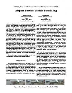
3. Problem Formulation 3.1. Problem Description. Let 𝐺 represent working service network. 𝑉 is the set of working service station set in the network 𝐺. We assume that time is divided into a set of discrete time periods 𝑇 = {𝑡 | 𝑡 = 1, . . . , 𝑀} where 𝑀 is the length of the planning horizon. We also assume that there exist demands for vehicle work service at terminal 𝑖, 𝑖 ∈ 𝑉, in period 𝑡, 𝑡 ∈ 𝑇. When vehicles serve demands, the revenues will generate. We assume a unit revenue per served demand in period 𝑡, denoted as 𝑎𝑡 . Serving demand results in the relocation of vehicles between various locations. It implies the need for redistribution of vehicles over the working service network from locations at which they have become idle to locations at which they can be reused. The minimum demands and maximum demands can be, respectively, represented as 𝑄𝑖𝑡min and 𝑄𝑖𝑡max at terminal 𝑖 in period 𝑡. These demands induce vehicles available to serve them. The minimum demands 𝑄𝑖𝑡min must be met, but maximum demands 𝑄𝑖𝑡max are not. If insufficient vehicles are available at location 𝑖 in period 𝑡 to meet maximum demand, the penalty cost for unmet demand will generate. We denote the unit penalty cost per period for unmet demand by 𝑏𝑡 . The level of demand in units of vehicle loads is assumed to be specified as data. We consider 𝜉 to be these demands which can be serviced by one vehicle. Let 𝑑𝑗𝑘 be the distance between any pair of terminal 𝑗 and 𝑘. The demand of terminal 𝑘 can be covered by vehicles located in 𝑗 if only the distance 𝑑𝑗𝑘 ≤ 𝐷, where 𝐷 is the maximum coverage distance. Considering the expense of purchasing or renting vehicle, we assume that the fixed costs of using vehicles are constant and denoted by 𝑐 for using one vehicle. The main purpose of the DWVS-DD is to propose working vehicle assignment plan for serving as many demands as possible in the given
4
Journal of Advanced Transportation Time period 1 1
Time period t 1
.. .
.. . GCH G;R QkM QkM
k .. .
k
.. .
dik ≤ D QitGCH QitG;R
i
.. .
N
1
.. .
k
···
.. .
Time period M
GCH G;R Qkt Qkt
.. . i
···
dik ≤ D G;R
GCH Qi1 Qi1
···
dik ≤ D .. . QGCH QkG;R t k t
i dik ≤ D .. . QGCH QG;R k M k M
k
.. .
.. .
N
N
Figure 1: Dynamic working service network with dual demands.
planning horizon at the highest possible profit. Owning or leasing a fleet of vehicles is generally quite costly, so it is natural to try to optimize the size of the required fleet. We emphasize the tradeoff among the investment for establishing a suitable fleet (i.e., the fixed cost), the benefits for meeting demands (i.e., the revenue for serving demands), and the loss of benefits for failing to satisfy demands (i.e., the penalty cost for unmet demands). Dynamic working service network with dual demands is shown in Figure 1. 3.2. Problem Definition and Notation. We assume that planning horizon is divided into a set of discrete instants 𝑇 = {𝑡 | 𝑡 = 1, . . . , 𝑀} where 𝑀 is the length of the planning horizon. A network is represented by graph 𝐺 = (𝑉, 𝐸) where 𝑉 is the set of terminal. 𝐸 is the set of link in the network. We present the complete notation for the problem here. Quickly summarizing the notation, we have the following decision variables: 𝑥𝑖𝑗𝑡 is the number of working vehicles dispatched from terminal 𝑖 to terminal 𝑗 in period 𝑡, 𝑖, 𝑗 ∈ 𝑁, 𝑡 ∈ 𝑇. 𝑈 is the vehicle fleet size.
be met. But the penalty cost for unmet demand will generate. Finally, the parameters are needed to describe the system: 𝜉 is these demands which can be serviced by one vehicle. 𝑑𝑗𝑘 is the distance between any pair of terminals 𝑗 and 𝑘. 𝐷 is the maximum coverage distance for any vehicle at any terminal. 𝛼𝑗𝑘 is 0-1 parameter. 𝛼𝑗𝑘 = 1 if the distance 𝑑𝑗𝑘 ≤ 𝐷, or 𝛼𝑗𝑘 = 0 otherwise. We assume that all parameters are deterministic and known. 3.3. Model Formulation. Given the above notations for the parameters and decision variables, we present the formulation as follows: [MIP] max
= 𝜉 ∑ ∑ ∑ 𝑎𝑡 𝑥𝑖𝑗𝑡
The revenues and costs associated with operating the system are as follows: 𝑎𝑡 is the revenue for one unit of met demands in period 𝑡. 𝑏𝑡 is the penalty cost for one unit of unmet demand in period 𝑡. 𝑐 is the fixed costs for one vehicle. In addition, the demand for vehicles is given by the following: 𝑄𝑖𝑡min is the minimum demand for working service at location 𝑖 in period 𝑡. The minimum demand must be satisfied by vehicles dispatched from other terminals. 𝑄𝑖𝑡max is the maximum demand for working service at location 𝑖 in period 𝑡. The maximum demand may not
The objective function (1) includes terms for revenues, penalty costs for unmet demand, and ownership cost for vehicles. It intends to maximize the total revenue of the system throughout the planning horizon. Constraint (2) restricts that the total number of working vehicle used cannot exceed the fleet size. Constraints (3) ensure that the minimum demand must be met. Constraints (4) impose an upper limit for the service capacity of the working vehicle at each location in each time period. Constraints (5) are coverage restriction and indicate the coverage relations between the demand nodes 𝑗 and candidate locations 𝑘, that is, 𝛼𝑗𝑘 = 1 if 𝑑𝑗𝑘 ⩽ 𝐷, or 𝛼𝑗𝑘 = 0 otherwise. Constraints (6) are conservation of flow constraints for vehicles at each location in each time period. Constraints (7) ensure that 𝑈 and 𝑥𝑗𝑖𝑡 are always nonnegative and integer. The nominal model of DWVS-DD can be solved as a mixed integer program (MIP) by CPLEX solver.
4. Reconstruction of the Model Using Preset Control Parameters We use 𝐸[𝐹𝑡+1 (𝑥)] to denote an expected value relative to 𝑥𝑡+1 . The expectation functional 𝐸[𝐹𝑡+1 (𝑥)] is called the stage 𝑡 expected recourse function. Now we introduce the expected recourse function into the MIP. The objective function can be expressed in the recursive form by
𝐸 [𝐹𝑡+1 (𝑥)] = ∑ 𝛿𝑗+1 𝑈𝑗,𝑡+1 .
(9)
𝑗∈𝐺
We also note that 𝑈𝑗,𝑡+1 = ∑ 𝑥𝑖𝑗𝑡 .
(10)
𝑖∈𝐺
Substituting them into 𝐸[𝐹𝑡+1 (𝑥)] gives 𝐸 [𝐹𝑡+1 (𝑥)] = ∑ 𝛿𝑗,𝑡+1 ∑ 𝑥𝑖𝑗𝑡 . 𝑗∈𝐺
𝑖∈𝐺
(11)
Substituting (11) into formula (8), we arrive at the local problem which is the problem to be solved at every time period. The new formulation of the local problem at single time period is represented as follows, called reconstruction model with single preset incremental parameters (RM-SPIP): [RM-SPIP] max
𝐹𝑡 (𝑥) = 𝜉 ∑ ∑ 𝑎𝑡 𝑥𝑖𝑗𝑡 𝑖∈𝐺 𝑗∈𝐺
max − ∑ 𝑏𝑡 (𝑄𝑗𝑡 − 𝜉 ∑ 𝑥𝑖𝑗𝑡 )
max 𝐹𝑡 (𝑥) = 𝜉 ∑ ∑ 𝑎𝑡 𝑥𝑖𝑗𝑡 𝑖∈𝐺 𝑗∈𝐺
𝑗∈𝐺
max − ∑ 𝑏𝑡 (𝑄𝑗𝑡 − 𝜉 ∑ 𝑥𝑖𝑗𝑡 ) − 𝑐 ⋅ 𝑈 𝑗∈𝐺
in each terminal grow linearly with the number of available vehicles. Here, we make substitution of expected recourse function by a linear function of marginal profit and vehicle number. We can now define the state of DWVS-DD at 𝑡th time period, that is, {𝑈𝑡 | 𝑈𝑗,𝑡 , 𝑗 ∈ 𝑁}. Note that the state of DWVS-DD at 𝑡th time period is given by the total vehicle supply in each terminal. By replacing the expectation recourse function 𝐸[𝐹𝑡+1 (𝑥)] with preset total incremental profit parameters 𝛿𝑗,𝑡+1 , the modified stage 𝑡 + 1 expected recourse function becomes
(8)
− 𝑐 ⋅ 𝑈 + ∑ 𝛿𝑗,𝑡+1 ∑ 𝑥𝑖𝑗𝑡 𝑗∈𝐺
𝑖∈𝐺
+ 𝐸 [𝐹𝑡+1 (𝑥)] . 4.1. Reconstruction of the Model with Single Preset Incremental Parameters 4.1.1. Preset Total Incremental Profit Parameters. We denote 𝛿𝑗,𝑡+1 as the total contribution of adding one loaded vehicle at terminal 𝑗 starting at 𝑡 + 1 time period, through the rest planning horizon. Because 𝛿𝑗,𝑡+1 depict the marginal profit of additional vehicle, we call them as preset incremental profit parameter (PIPP). 4.1.2. Reconstruction Model with Single Preset Incremental Parameters. It is common sense that the total expected profits in each terminal at each time period depend on the number of available vehicles there. Thus, the total expected profits
𝑖∈𝐺
(12)
𝑖∈𝐺
= ∑ ∑ (𝑎𝑡 𝜉 + 𝑏𝑡 𝜉 + 𝛿𝑗,𝑡+1 ) 𝑥𝑖𝑗𝑡 𝑖∈𝐺 𝑗∈𝐺
max − ∑ 𝑏𝑡 𝑄𝑗𝑡 −𝑐⋅𝑈 𝑗∈𝐺
s.t. Constraints (2)–(7). 4.2. Reconstruction of the Model with Double Preset Incremental-Decremental Parameters + 4.2.1. Preset Incremental Revenue Parameters. Let 𝛿𝑗,𝑡+1 be the revenue of adding one vehicle to servicing demand at terminal 𝑗 starting at 𝑡 + 1 time period, through the rest + planning horizon. Because 𝛿𝑗,𝑡+1 depict the marginal revenue of additional vehicle, we call them as preset incremental revenue parameter (PIRP).
6
Journal of Advanced Transportation
4.2.2. Preset Decremental Cost Parameters. The same − approach is adopted. We denote 𝛿𝑗,𝑡+1 as the effect on penalty cost of adding one vehicle to servicing demand at terminal 𝑗 starting at 𝑡 + 1 time period, through the rest planning − horizon. Because 𝛿𝑗,𝑡+1 depict the marginal penalty cost of additional vehicle, we call them as preset decremental cost parameter (PDCP). 4.2.3. Reconstructing Model with Double Preset IncrementalDecremental Parameters. By replacing the expectation recourse function 𝐸[𝐹𝑡+1 (𝑥)] with double preset incremental+ − and 𝛿𝑗,𝑡+1 , the modified stage decremental parameters 𝛿𝑗,𝑡+1 𝑡 + 1 expected recourse function becomes + − 𝐸 [𝐹𝑡+1 (𝑥)] = ∑ 𝛿𝑗,𝑡+1 𝑈𝑗,𝑡+1 + ∑ 𝛿𝑗,𝑡+1 𝑈𝑗,𝑡+1 . 𝑗∈𝐺
𝑗∈𝐺
Virtual time period 1
G;R GCH Qk1 Qk1
𝐸 [𝐹𝑡+1 (𝑥)] = ∑
𝑗∈𝐺
∑ 𝑥𝑖𝑗𝑡 + ∑
𝑖∈𝐺
𝑗∈𝐺
− 𝛿𝑗,𝑡+1
∑ 𝑥𝑖𝑗𝑡 .
𝑖∈𝐺
.. .
s
.. . k
dik ≤ D QkG;R QkGCH 1 1
Uk ,1
UN,1
N
(14)
Figure 2: Dynamic working network for virtual time period.
5.1. Procedure of the Sampling Data 5.1.1. Determining Initial Vehicle Distribution Step 1.1. Since all minimum demand and maximum demand min max are available for the first time, we have 𝑄𝑖,1 and 𝑄𝑖,1 .
= 𝜉 ∑ ∑ 𝑎𝑡 𝑥𝑖𝑗𝑡
Step 1.2. Add a virtual source terminal 𝑆 into working service network 𝐺(𝑉, 𝐸). In Figure 2, there are only the outbound arcs for source terminal 𝑆. The formulation of local problem for virtual time period is denoted as LP-VTP. This model includes the following objective function and constraints:
𝑖∈𝐺 𝑗∈𝐺
max − ∑ 𝑏𝑡 (𝑄𝑗𝑡 − 𝜉 ∑ 𝑥𝑖𝑗𝑡 ) 𝑗∈𝐺
𝑖∈𝐺
+ − 𝑐 ⋅ 𝑈 + ∑ 𝛿𝑗,𝑡+1 ∑ 𝑥𝑖𝑗𝑡 𝑗∈𝐺
𝑗∈𝐺
Ui,1
i
.. .
𝐹𝑡 (𝑥)
+∑
dik ≤ D GCH G;R Qi1 Qi1
(13)
Substituting (14) into formula (8), we arrive at the local problem for each time period. The model can be reformulated in piecewise form as follows. We name this new form as reconstruction model with double preset incrementaldecremental parameters (RM-DPIDP). [RM-DPIDP] max
Uk,1
k
And 𝑈𝑗,𝑡+1 = ∑𝑖∈𝐺 𝑥𝑖𝑗𝑡 , 𝐸[𝐹𝑡+1 (𝑥)] can be written as + 𝛿𝑗,𝑡+1
5. Approach for Preset Control Parameter The preset control parameter results in decoupling the problems for different time period. In section, we will develop an interactive procedure to provide approximations of the preset control parameters.
(16)
𝑘∈𝐺
𝑈, 𝑥𝑠𝑖0 ≥ 0, and integer
∀𝑖 ∈ 𝐺.
Because we pose this local problem in the format of an integer linear program, CPLEX solver can be used. Optimal solutions 𝑥𝑠𝑖0 can be obtained by using CPLEX for solving LPVTP. Step 1.3. Initial vehicle distribution is obtained according to 𝑈𝑖,1 = 𝑥𝑠𝑖0 .
Journal of Advanced Transportation
7
5.1.2. Sampling Data with Solving Local Problem. By solving local problem at each time period, the data can be obtained. The procedure of sampling data procedure is explained as follows. Step 2.1. The state vector, that is, {𝑈𝑡 | 𝑈𝑖𝑡 , 𝑖 ∈ 𝐺}, is updated by equation 𝑈𝑖𝑡 = ∑𝑗∈𝐺 𝑥𝑗𝑖,(𝑡−1) . Step 2.2. Since minimum demand and maximum demand are deterministic and known for the whole planning horizon, we min max and 𝑄𝑗,𝑡+1 . have 𝑄𝑗,𝑡+1 Step 2.3. Solve local problem (LP), one for each time period, by CPLEX solver to obtain optimal solution 𝑥𝑖𝑗𝑡 . The formulation of the LP is shown as follows: [LP] max 𝐹𝑡 = 𝜉 ∑ 𝑎𝑡 𝑈𝑖𝑡 − ∑ 𝑏𝑡 (𝑄𝑖𝑡max − 𝜉𝑈𝑖𝑡 ) 𝑖∈𝐺
𝑖∈𝐺
− 𝑐 ∑ 𝑈𝑖𝑡 𝑖∈𝐺
∀𝑖 ∈ 𝐺
min , 𝜉 ∑ 𝑥𝑖𝑗𝑡 ≥ 𝑄𝑗,𝑡+1
𝜉 ∑ 𝑥𝑖𝑗𝑡 ≤ ∑
∀𝑗 ∈ 𝐺
𝑘∈𝐺
max 𝛼𝑗𝑘 𝑄𝑘,𝑡+1 ,
5.2.2. Coupled Correlation Function with Double Preset Control Parameters (CCF-DPCP). The coupled correlation is set up in a control theoretic setting. The pair {𝐹𝑖𝑡+ , 𝐹𝑖𝑡− } represents the system outputs. The set {𝑈𝑖𝑡 , 𝑄𝑖𝑡min , 𝑄𝑖𝑡max } represents the system inputs. Multi-input and multi-output control systems are set up. We generate a quadratic polynomial equation for the effect of vehicle supply, minimum demand, and maximum demand on the revenue and penalty cost in each terminal where the function is used to approximate the incremental revenue parameter and decremental cost parameters of RM-DPIDP. The quadratic polynomial function for approximating the double preset incremental-decremental parameters of RM-DPIDP has the form as follows: 𝐹𝑖+ (𝑈𝑖 , 𝑄𝑖min , 𝑄𝑖max )
Step 2.4. Taking optimal solution 𝑥𝑖𝑗𝑡 into the objective function of local problem, {𝐹𝑖𝑡 , 𝐹𝑖𝑡+ , 𝐹𝑖𝑡− } can be obtained, where {𝐹𝑖𝑡 , 𝐹𝑖𝑡+ , 𝐹𝑖𝑡− } denotes, respectively, total profit, revenue, and penalty cost for each time period. Step 2.5. Record these data, that is, {𝑈𝑖𝑡 , 𝑄𝑖𝑡min , 𝑄𝑖𝑡max , 𝐹𝑖𝑡 , 𝐹𝑖𝑡+ , 𝐹𝑖𝑡− }. 5.2. Modeling for Coupled Correlation 5.2.1. Coupled Correlation Function with Single Preset Control Parameters (CCF-SPCP). The total profit function is a function of vehicle supply, minimum demand, and maximum demand. We generate a quadratic polynomial function for the effect of vehicle supply, minimum demand, and maximum demand on the total profits in each terminal where the function is used to approximate the incremental profit parameter of RM-SPIP. The quadratic polynomial function for approximating the single preset incremental parameter of RM-SPIP has the following form: [CCF-SPCP] 𝐹𝑖 (𝑈𝑖 , 𝑄𝑖min , 𝑄𝑖max ) 2
Above coupled correlation function with single preset control parameters is denoted as CCF-SPCP.
+ 𝛾𝑖3 (𝑄𝑖max ) + 𝛾𝑖4 𝑈𝑖 𝑄𝑖min + 𝛾𝑖5 𝑈𝑖 𝑄𝑖max + 𝛾𝑖6 𝑄𝑖min 𝑄𝑖max + 𝛾𝑖7 𝑈𝑖 + 𝛾𝑖8 𝑄𝑖min + 𝛾𝑖9 𝑄𝑖max + 𝛾𝑖10 , 𝑖 ∈ 𝐺. Above coupled correlation function with double preset control parameters is denoted as CCF-DPCP. 5.3. Fitting Parameters of Coupled Correlation Function 5.3.1. Sampling Data Sets for Fitting Parameters. By solving local problem at each time period, the data sets can be obtained. Solution of local problem, that is, 𝑥𝑖𝑗𝑡 , is obtained by CPLEX solver. {𝐹𝑖𝑡 , 𝐹𝑖𝑡+ , 𝐹𝑖𝑡− } is carried on by taking 𝑥𝑖𝑗𝑡 into the objective function of local problem. State vector {𝑈𝑖𝑡 } is obtained by updated approach of local problem. In order to fit parameters of coupled correlation function, these data are split into three data sets, that is, {𝐹𝑖𝑡 , 𝑈𝑖𝑡 , 𝑄𝑖𝑡min , 𝑄𝑖𝑡max | 𝑖 ∈ 𝐺, 𝑡 ∈ 𝑇}, {𝐹𝑖𝑡+ , 𝑈𝑖𝑡 , 𝑄𝑖𝑡min , 𝑄𝑖𝑡max | 𝑖 ∈ 𝐺, 𝑡 ∈ 𝑇}, and {𝐹𝑖𝑡− , 𝑈𝑖𝑡 , 𝑄𝑖𝑡min , 𝑄𝑖𝑡max | 𝑖 ∈ 𝐺, 𝑡 ∈ 𝑇}.
8
Journal of Advanced Transportation
5.3.2. Fitting the Parameters of Coupled Correlation Function. We use the data set {𝐹𝑖𝑡 , 𝑈𝑖𝑡 , 𝑄𝑖𝑡min , 𝑄𝑖𝑡max | 𝑖 ∈ 𝐺, 𝑡 ∈ 𝑇} to fit the parameter of RM-SPIP with regression method. Thus these parameters {𝛼𝑖𝑚 | 𝑖 ∈ 𝐺, 𝑚 = 1, . . . , 10} are derived. The coupled correlation function CCF-SPCP is obtained. Again, using the same approach, we introduce the data sets {𝐹𝑖𝑡+ , 𝑈𝑖𝑡 , 𝑄𝑖𝑡min , 𝑄𝑖𝑡max | 𝑖 ∈ 𝐺, 𝑡 ∈ 𝑇} and {𝐹𝑖𝑡− , 𝑈𝑖𝑡 , 𝑄𝑖𝑡min , 𝑄𝑖𝑡max | 𝑖 ∈ 𝐺, 𝑡 ∈ 𝑇} into the RM-DPIDP for fitting these parameters {𝛽𝑖𝑚 | 𝑖 ∈ 𝐺, 𝑚 = 1, . . . , 10} and {𝛽𝑖𝑚 | 𝑖 ∈ 𝐺, 𝑚 = 1, . . . , 10}. The coupled correlation function CCF-DPCP is obtained. 5.4. Computing the Preset Control Parameters of Coupled Correlation Function 5.4.1. Computing Single Preset Control Parameter with CCFSPCP. The coupled correlation function CCF-SPCP implies the effect of vehicle supply 𝑈𝑗 , minimum demand 𝑄𝑗min , and maximum demand 𝑄𝑗max on the profits 𝐹𝑗 . As the derivative of 𝐹𝑗 (𝑈𝑗 , 𝑄𝑗min , 𝑄𝑗max ) with respect to 𝑈𝑗 shows the effect of adding one vehicle in 𝑗 terminal at 𝑡 + 1 time period through the rest the planning horizon, 𝛿𝑗,𝑡+1 is given by
min max = 2𝛽𝑗1 𝑈𝑗,𝑡+1 + 𝛽𝑗4 𝑄𝑗,𝑡+1 + 𝛽𝑗5 𝑄𝑗,𝑡+1 + 𝛽𝑗7 .
Correspondingly, as the derivative of 𝐹𝑗− (𝑈𝑗 , 𝑄𝑗min , 𝑄𝑗max ) with respect to 𝑈𝑗 nicely depicts the effect of adding one vehicle in 𝑗 terminal at 𝑡 + 1 time period through the rest the − is written as planning horizon, 𝛿𝑗,𝑡+1 𝑄𝑗 =𝑄𝑗,𝑡+1 ,𝑄𝑗 𝜕𝐹𝑗− (𝑈𝑗 , 𝑄𝑗min , 𝑄𝑗max ) = 𝜕𝑈𝑗 𝑈𝑗 =𝑈𝑗,𝑡+1 min
− 𝛿𝑗,𝑡+1
min
max
max =𝑄𝑗,𝑡+1
.
(24)
Accordingly, the solution approach of preset decremental cost parameter (PDCP) is shown in the following formula:
min max = 2𝛾𝑗1 𝑈𝑗,𝑡+1 + 𝛾𝑗4 𝑄𝑗,𝑡+1 + 𝛾𝑗5 𝑄𝑗,𝑡+1 + 𝛾𝑗7 .
𝑗,𝑡+1
6. Piecewise Method by Updating Preset Control Parameters
min max = 2𝛼𝑗1 𝑈𝑗,𝑡+1 + 𝛼𝑗4 𝑄𝑗,𝑡+1 + 𝛼𝑗5 𝑄𝑗,𝑡+1 + 𝛼𝑗7 .
5.4.2. Computing Double Preset Control Parameter with CCFDPCP. We use the same approach to compute the double preset control parameter of coupled correlation function CCF-DPCP. The coupled correlation function implies the effect of vehicle supply 𝑈𝑗 , minimum demand 𝑄𝑗min and maximum demand 𝑄𝑗max on revenue 𝐹𝑗+ and penalty cost 𝐹𝑗− . As the derivative of 𝐹𝑗+ (𝑈𝑗 , 𝑄𝑗min , 𝑄𝑗max ) with respect to 𝑈𝑗 shows the effect of adding one vehicle in 𝑗 terminal at 𝑡 + 1 + is time period through the rest the planning horizon, 𝛿𝑗,𝑡+1 given by + 𝛿𝑗,𝑡+1
In this section, we develop a solution approach based on updating preset control parameters. An overview of the framework of piecewise method by updating preset control parameters (PM-PCP) is explained as follows. Stage 1 (sampling data sets). Step 1.1. Add a virtual source terminal into working service network. The formulation of local problem for virtual time period is written. Optimal solutions 𝑥𝑠𝑖0 can be obtained by using CPLEX for solving local problem. Then initial vehicle distribution {𝑈𝑖,1 | 𝑖 ∈ 𝐺} is obtained. Step 1.2. By solving local problem (LP) at each time period with CPLEX solver, optimal solutions 𝑥𝑖𝑗𝑡 can be obtained. Taking optimal solution 𝑥𝑖𝑗𝑡 into the objective function of
Journal of Advanced Transportation local problem, {𝐹𝑖𝑡 , 𝐹𝑖𝑡+ , 𝐹𝑖𝑡− } can be obtained. State vector {𝑈𝑖𝑡 } is obtained by updated approach of local problem. Step 1.3. Record these data sets {𝑈𝑖𝑡 , 𝑄𝑖𝑡min , 𝑄𝑖𝑡max , 𝐹𝑖𝑡 , 𝐹𝑖𝑡+ , 𝐹𝑖𝑡− } in each terminal at each time period. Step 1.4. As such, repeat Steps 1.1 to 1.3 for the whole planning horizon. In order to fit parameters of coupled correlation function, these data are split into three data sets, that is, {𝐹𝑖𝑡 , 𝑈𝑖𝑡 , 𝑄𝑖𝑡min , 𝑄𝑖𝑡max | 𝑖 ∈ 𝐺, 𝑡 ∈ 𝑇}, {𝐹𝑖𝑡+ , 𝑈𝑖𝑡 , 𝑄𝑖𝑡min , 𝑄𝑖𝑡max | 𝑖 ∈ 𝐺, 𝑡 ∈ 𝑇}, and {𝐹𝑖𝑡− , 𝑈𝑖𝑡 , 𝑄𝑖𝑡min , 𝑄𝑖𝑡max | 𝑖 ∈ 𝐺 𝑡 ∈ 𝑇}. Stage 2 (coupled correlation formulation). Step 2.1. Using the data set {𝐹𝑖𝑡 , 𝑈𝑖𝑡 , 𝑄𝑖𝑡min , 𝑄𝑖𝑡max | 𝑖 ∈ 𝐺, 𝑡 ∈ 𝑇} to fit these parameters of CCF-SPCP by regression method, the coupled correlation function CCF-SPCP is formed. Step 2.2. Using the data sets {𝐹𝑖𝑡+ , 𝑈𝑖𝑡 , 𝑄𝑖𝑡min , 𝑄𝑖𝑡max | 𝑖 ∈ 𝐺, 𝑡 ∈ 𝑇} and {𝐹𝑖𝑡+ , 𝑈𝑖𝑡 , 𝑄𝑖𝑡min , 𝑄𝑖𝑡max | 𝑖 ∈ 𝐺, 𝑡 ∈ 𝑇} to fit these parameters of CCF-DPCP by regression method, the coupled correlation function CCF-DPCP is formed. Stage 3 (piecewise method guided by preset control parameters). Step 3.1. Single preset control parameters of RM-SPIP 𝛿𝑗,𝑡+1 are computed by formula (21). Step 3.2. Taking incremental profit parameters 𝛿𝑗,𝑡+1 into the objective function of MIP, the piecewise form of the model new is obtained by (RM-SPIP) is given. The new solution 𝑥𝑖𝑗𝑡 resolving RM-SPIP using CPLEX solver for the beginning of the 1st period until the end of an appropriate planning horizon 𝑀. Further, 𝑈𝑖𝑡new are obtained. Step 3.3. Double preset control parameters of RM-DPIDP + − and 𝛿𝑗,𝑡+1 are computed by formulas (23) and (25). 𝛿𝑗,𝑡+1 + Step 3.4. Taking preset incremental revenue parameter 𝛿𝑗,𝑡+1 − and preset decremental cost parameter 𝛿𝑗,𝑡+1 into the objective function of MIP, the piecewise form of the model (RMnew DPIDP) is given. The new solution 𝑥𝑖𝑗𝑡 is obtained by resolving RM-DPIDP using CPLEX solver for the beginning of the 1st period until the end of an appropriate planning horizon 𝑀. Further, 𝑈𝑖𝑡new are obtained.
7. Numerical Study In this section, we try to evaluate the quality of the PMPCP method in terms of traditional measure such as objective function and execution time. Section 7.1 describes the experimental design, and Sections 7.2–7.5 report the numerical results. 7.1. Instances and Test Settings. This section describes the data used in the numerical testing of the models. For each vehicle, the region and the time of first availability have to be known. In this data set, the working service network is composed of 10
9 terminals and of fixed-length links joining them. The length of the planning horizon is 50-time period. The length of each time period is constant 60-time unit. All vehicles are assumed to be of the same type and all demands can be met from that type of vehicle. The minimum demands at each terminal are assumed to follow Poisson distributions with mean 250. The maximum demands at each terminal are assumed to follow Poisson distributions with mean 400. The revenue for one unit of met demands is 40 dollar. The penalty cost for one unit of unmet demand is 18 dollar. The fixed cost for owning or leasing vehicle is 50,000 dollar per vehicle. The demands which can be serviced by vehicle are 100 units per vehicle. The distance between any pair of terminal are assumed to uniform distributions with mean 300. The maximum coverage distance for any vehicle at any terminal is 500 meters. In the following, the PM-PCP program for RM-SPIP and RM-DPIDP is coded by using MATLAB 2014 Edition. A Pentium IV 3.4 GHz processor with 2 GB memory is used for the computation. For solving the MIP, CPLEX solver is also used. We compare the three models using the test instances and evaluate the performance of the MIP model, RM-SPIP model, and RM-DPIDP model. 7.2. Performance Evaluation. In this section, the major criterion in assessing the performance of the models MIP, RMSPIP, and RM-DPIDP is the profit generated by revenues for assigning vehicles, penalty costs for unmet demand, and ownership costs for owning vehicle in planning horizon. The PM-PCP procedure is coded by using MATLAB 2014 Edition to solve the RM-SPIP and RM-DPIDP. The MIP model is solved by CPLEX. In the experiment, we test the performance of the solution procedure on working service network. At each iteration, the objective function value for each time period is recorded. When the models MIP, RM-SPIP, and RM-DPIDP are compared, the difference in total profit is very clear. The RMSPIP and RM-DPIDP model can generate higher the total profit than MIP model. Furthermore, we observe that the solution obtained from RM-DPIDP outperforms the solution approaches from RM-SPIP. The results obtained by RMDPDIP, RM-SPIP, and MIP are displayed in Figure 3. 7.3. Evolution of the Preset Control Parameters. The preset control parameters are important for the RM-SPIP model and RM-DPIDP model. In this section, we indicate the evolution of the preset control parameters for whole planning horizon. For the RM-SPIP model and RM-DPIDP model, the following preset control parameters are reported: preset incremental profit parameter (PIPP) for RM-SPIP model and preset incremental revenue parameter (PIRP) and preset decremental cost parameter (PDCP) for RM-DPIDP model. Figure 4 shows the evolution of three types preset control parameters through 50-time period. 7.4. Numerical Results on Instances for Different Length of Planning Horizon. In this section, we use two measures of performance. The first one is the OPT, which is the value of
10
Journal of Advanced Transportation Table 1: Performance for MIP, RM-SPIP, and RM- DPIDP model applied to different working service station size.
Number of service station 3 5 8 10 13 15 18 20 23 25 28 30 33 35 38 40 43 45 48 50
period), the solution of RM-SPIP and RM-DPIDP model can obviously maintain higher total profits than that of MIP. The OPT performance is shown in Figure 5. Additional measures are the CPU time. The required CPU time is reported to indicate the usefulness of models MIP, RM-SPIP, and RM-DPIDP. These times include the processing time needed to solve the RM-SPIP and RMDPIDP model by PM-PCP program and solve the MIP model by CPLEX program. The computational results of the performance of the models are shown in Figure 6.
Figure 3: Comparison of models RM-DPDIP, RM-SPIP, and MIP.
the objective function obtained by the MIP and the optimal value obtained by RM-SPIP and RM-DPIDP. The second measure of performance is the CUP time to run CPLEX solver for MIP model and the PM-PCP program for RM-SPIP model and RM-DPIDP model. Dynamic working vehicle scheduling with dual demands service network (DWVS-DD) for different length of planning horizon is, respectively, solved by models MIP, RM-SPIP, and RM-DPIDP. For small time period size (up to 5 time period), the solving RM-SPIP and RM-DPIDP model can generally result in slightly higher total profits than that of MIP model. Nevertheless for bigger time period size (up to 50 time
7.5. Numerical Results on Instances for Working Service Station Size. In this section, two measures of performance are adopted. The first one is the OPT difference, which is the difference between the value of the objective function obtained by MIP model and the optimal value obtained by RM-SPIP and RM-DPIDP model. The second measure of performance is the CUP time difference, which is the difference between the CPU time to find the optimal solution of MIP model by using CPLEX solver and the CPU time to run the PM-PCP program for RM-SPIP and RM-DPIDP model. When the models MIP, RM-SPIP, and RM-DPIDP are compared, the difference in total profit is very clear. Meanwhile, the OPT difference will increase with the working service station size. In other words, with increasing working service station size, the OPT difference will also increase. The results for the OPT difference of different working service station size are listed in Table 1. Furthermore, we have to look at the following affect in CPU time difference. Here DWVS-DD size is described by
11
×103 7
×103 8.5
Preset incremental revenue parameter
Preset incremental profit parameter
Journal of Advanced Transportation
6.5 6 5.5 5 4.5 4
0
5
10
15
20 25 30 Time period
35
40
45
50
(a) Single preset parameters (preset incremental profit parameter)
Figure 4: Dynamic change of preset increment parameters.
900
×105 8
800 700 RM-DPIDP
6
Computer time
Cumulative total profit
7
5 RM-SPIP
4 3
MIP
500 RM
300
0 0
5
10
15
20 25 30 Time period
35
40
45
50
Figure 5: The OPT performance of 3 models for different length of planning horizon.
working service station size. The CUP time difference for different DWVS-DD size is described in Table 1. Using polynomial curve fitting to the OPT data can provide good results. The results are shown in Figure 7. Referring to the results obtained by using the PM-PCP
IP
SP
RM
MIP
100
1
P
ID
DP
400 200
2
0
600
0
5
10
15
20
25
30
35
40
45
50
Time period
Figure 6: CPU time of 3 models for different length of planning horizon.
program for RM-SPIP and RM-DPIDP model, we observe that the quality of the OPT value is improved. In comparison, the performance of PM-PCP program for RM-SPIP and RMDPIDP is very significant when the scale of the problem becomes relatively large.
12
Journal of Advanced Transportation ×106 3
OPT difference
2.5 2 1.5 1 0.5 0
0
5
10
15 20 25 30 35 Working service station size
40
45
50
Fitting curve for OPT of MIP Fitting curve for OPT of RM-SPIP Fitting curve for OPT of RM-DPIDP
Conflicts of Interest The authors declare that there are no conflicts of interest regarding the publication of this paper.
Figure 7: Fitting curve of OPT for 3 models. ×102 18
Acknowledgments This research is supported by National Natural Science Foundation of China (Grant no. U1604150) and Humanities & Social Sciences Research Foundation of Ministry of Education of China (Grant no. 15YJC630148). The support is gratefully acknowledged.
16 14 CPU time
reformulated as a piecewise form, namely, RM-SPIP and RM-DPIDP. According to the specific structure of the RMSPIP and RM-DPIDP, piecewise method by updating preset control parameters (PM-PCP) is developed. The primary goal of this paper is to set up a new model of the DWVS-DD and solve it in an effective and efficient way. Tests have been conducted to examine the performance of the PM-PCP program for the proposed new model. Future research can focus on multiple vehicle and service types. The assumption of multiple vehicle and service types adds considerable complexity to the problem of DWVS-DD. In spite of this, we have shown that the PM-PCP approach can handle very big problems and provide high-quality integer solutions.
12 10 8
References
6
[1] Y. M. Hou, Z. H. Jia, X. Tian, and F. F. Wei, “Research on vehicle routing problem with soft time windows,” Journal of Systems Engineering, vol. 30, no. 2, pp. 240–250, 2015. [2] X. X. Cao, J. F. Tang, and L. L. Liu, “An accurate algorithm based on set partitioning for airport shuttle vehicle scheduling problem,” Systems Engineering Theory and Practice, vol. 33, no. 7, pp. 1682–1689, 2013. [3] K. Li, L. X. Tang, and S. F. Chen, “Modeling and optimization of spatial allocation and vehicle scheduling problem in multi container yard,” System Engineering Theory and Practice, vol. 34, no. 1, pp. 115–121, 2014. [4] S. Dabia, S. Ropke, T. Van Woensel, and T. De Kok, “Branch and price for the time-dependent vehicle routing problem with time windows,” Transportation Science, vol. 47, no. 3, pp. 380– 396, 2011. [5] J. Han, C. Lee, and S. Park, “A robust scenario approach for the vehicle routing problem with uncertain travel times,” Transportation Science, vol. 48, no. 3, pp. 373–390, 2014. [6] I. Muter, J.-F. Cordeau, and G. Laporte, “A branch-and-price algorithm for the multidepot vehicle routing problem with interdepot routes,” Transportation Science, vol. 48, no. 3, pp. 425–441, 2014. [7] T. Vidal, T. G. Crainic, M. Gendreau, and C. Prins, “A unified solution framework for multi-attribute vehicle routing problems,” European Journal of Operational Research, vol. 234, no. 3, pp. 658–673, 2014. [8] M. Battarra, G. s. Erdo˘gan, and D. Vigo, “Exact algorithms for the clustered vehicle routing problem,” Operations Research, vol. 62, no. 1, pp. 58–71, 2014.
4
0
5
10
15 20 25 30 35 Working service station size
40
45
50
Fitting curve for CPU time of MIP Fitting curve for CPU time of RM-SPIP Fitting curve for CPU time of RM-DPIDP
Figure 8: Fitting curve of CUP time for 3 models.
Furthermore, using polynomial curve fitting to the CUP time data can also provide good results. The results are displayed in Figure 8. In comparison, along with the increase in scale of the problem, CPU time of PM-PCP program for RM-SPIP and RM-DPIDP slightly increases.
8. Conclusions In this paper, a mixed integer programming model has been developed for DWVS-DD. Instead of a large integer program, the problem is decomposed into small local problems that are guided by preset control parameters. The preset control parameters result in decoupling the local problems for different time periods. Then we propose two types of preset control parameters, namely, single preset control parameters (SPCP) and double preset control parameters (DPCP). By introducing them into the MIP model, the models are then
Journal of Advanced Transportation [9] J. Zak, A. Redmer, and P. Sawicki, “Multiple objective optimization of the fleet sizing problem for road freight transportation,” Journal of Advanced Transportation, vol. 45, no. 4, pp. 321–347, 2011. [10] A. Shyshou, I. Gribkovskaia, and J. Barcel´o, “A simulation study of the fleet sizing problem arising in offshore anchor handling operations,” European Journal of Operational Research, vol. 203, no. 1, pp. 230–240, 2010. [11] A. Rahimi-Vahed, T. G. Crainic, M. Gendreau, and W. Rei, “Fleet-sizing for multi-depot and periodic vehicle routing problems using a modular heuristic algorithm,” Computers & Operations Research, vol. 53, pp. 9–23, 2015. [12] K. Ertogral, A. Akbalik, and S. Gonz´alez, “Modelling and analysis of a strategic fleet sizing problem for a furniture distributor,” European Journal of Industrial Engineering, vol. 11, no. 1, pp. 49–77, 2017. [13] A. Ferrara, E. Gebennini, and A. Grassi, “Fleet sizing of laser guided vehicles and pallet shuttles in automated warehouses,” International Journal of Production Economics, vol. 157, no. 1, pp. 7–14, 2014. [14] K.-H. Chang, Y.-H. Huang, and S.-P. Yang, “Vehicle fleet sizing for automated material handling systems to minimize cost subject to time constraints,” IIE Transactions (Institute of Industrial Engineers), vol. 46, no. 3, pp. 301–312, 2014. [15] J. A. Barrios and J. D. Godier, “Fleet sizing for flexible carsharing systems simulation-based approach,” Transportation Research Record, vol. 2416, pp. 1–9, 2014. [16] C ¸ . Koc¸, T. Bektas, O. Jabali, and G. Laporte, “The fleet size and mix location-routing problem with time windows: formulations and a heuristic algorithm,” European Journal of Operational Research, vol. 248, no. 1, pp. 33–51, 2016. [17] S. J. Park and D. S. Kim, “Container fleet-sizing for part transportation and storage in a two-level supply chain,” Journal of the Operational Research Society, vol. 66, no. 9, pp. 1442–1453, 2015. [18] J. Xia, K. X. Li, H. Ma, and Z. Xu, “Joint planning of fleet deployment, speed optimization, and cargo allocation for liner shipping,” Transportation Science, vol. 49, no. 4, pp. 922–938, 2015. [19] J. P. Pita, N. Adler, and A. P. Antunes, “Socially-oriented flight scheduling and fleet assignment model with an application to Norway,” Transportation Research Part B: Methodological, vol. 61, pp. 17–32, 2014. [20] V. L. Pilla, J. M. Rosenberger, V. Chen, N. Engsuwan, and S. Siddappa, “A multivariate adaptive regression splines cutting plane approach for solving a two-stage stochastic programming fleet assignment model,” European Journal of Operational Research, vol. 216, no. 1, pp. 162–171, 2012. [21] Z. Liang and W. A. Chaovalitwongse, “A network-based model for the integrated weekly aircraft maintenance routing and fleet assignment problem,” Transportation Science, vol. 47, no. 4, pp. 493–507, 2012. [22] H. D. Sherali, K.-H. Bae, and M. Haouari, “An integrated approach for airline flight selection and timing, fleet assignment, and aircraft routing,” Transportation Science, vol. 47, no. 4, pp. 455–476, 2013. ´ [23] K. Tierney, B. Askelsd´ ottir, R. M. Jensen, and D. Pisinger, “Solving the liner shipping fleet repositioning problem with cargo flows,” Transportation Science, vol. 49, no. 3, pp. 652–674, 2015. [24] A. S. Hashemi and J. Sattarvand, “Simulation based investigation of different fleet management paradigms in open pit
13
[25]
[26]
[27]
[28]
[29]
[30]
[31]
mines-a case study of Sungun copper mine,” Archives of Mining Sciences, vol. 60, no. 1, pp. 195–208, 2015. J. T. Lin, C. H. Wu, and C. W. Huang, “Dynamic vehicle allocation control for automated material handling system in semiconductor manufacturing,” Computers & Operations Research, vol. 40, no. 10, pp. 2329–2339, 2013. H. P. Sim˜ao, J. Day, A. P. George, T. Gifford, J. Nienow, and W. B. Powell, “An approximate dynamic programming algorithm for large-scale fleet management: A case application,” Transportation Science, vol. 43, no. 2, pp. 178–197, 2009. H. Topaloglu and W. Powell, “Incorporating pricing decisions into the stochastic dynamic fleet management problem,” Transportation Science, vol. 41, no. 3, pp. 281–301, 2007. B. Li, H. Xuan, and J. Li, “Alternating solution strategies of bilevel programming model for stochastic dynamic fleet scheduling problem with variable period and storage properties,” Kongzhi yu Juece/Control and Decision, vol. 30, no. 5, pp. 807– 814, 2015. B. Li, H. Xuan, and J. Li, “Solving strategies for the stochastic dynamic fleet scheduling problem based on leading of parameters,” Journal of Systems Engineering, vol. 31, no. 4, pp. 545–556, 2016. B. Li and H. Xuan, “Solving strategy for stochastic dynamic fleet scheduling with station operation coordination,” Kongzhi yu Juece/Control and Decision, vol. 32, no. 1, pp. 71–78, 2017. M.-J. Yao and J.-Y. Huang, “Scheduling of transportation fleet maintenance service by an improved Lipschitz optimization algorithm,” Optimization Methods & Software, vol. 29, no. 3, pp. 592–609, 2014.