765
SHIP SCHEDULING AND SERVICE NETWORK INTEGRATION FOR LINER SHIPPING COMPANIES AND STRATEGIC ALLIANCES Shih-Chan TING Assistant Professor, Kai Nan University Ph.D. Candidate Institution of Traffic and Transportation National Chiao Tung University 114, Sec.1, Chung-Hsiao West Road, Taipei 100, Taiwan Fax: +886-3-341-2361 E-mail:
[email protected]
Gwo-Hshiung TZENG Professor Institute of Technology Management National Chiao Tung University 1001, Ta-Hsueh Road, Hsinchu 300, Taiwan Fax: +886-2-2312-0519 E-mail:
[email protected]
Abstract: Liner shipping companies and strategic alliances can benefit greatly from using systematic methods to streamline their operations, thus it is highly desirable to improve ship scheduling on service route planning and integrate their service networks by analytical models. The purpose of this study is to propose a dynamic programming (DP) model for ship scheduling for planning a service route. This can help planners make better scheduling decisions under berth time-window constraints. The proposed model derives an optimal scheduling strategy including cruising speed and quay crane dispatching decisions, rather than a tentative and rough schedule arrangement. The proposed model is extended to cases of integrating one company’s or strategic alliance partners’ service networks to gain more efficient hub-and-spoke operations, tighter transshipment and better level-of-service. Key Words: liner shipping, ship scheduling, network integration, dynamic programming
1. INTRODUCTION Liner shipping provides regular services between specified ports according to timetables advertised in advance. The services are, in principle, open to all shippers and seem like public transport services. The provision of such services, often offering global or regional coverage, requires extensive infrastructure in terms of ships, equipment (e.g. containers, chassis, trailers) and needed to appoint agents at each calling port for the services. Since a service route of one containership fleet, once determined, is hard to alter for a certain period of time, the initial route planning and scheduling decisions should be made carefully after thorough study and planning. It is highly desirable to plan new routes and rearrange service networks by analytical methods, since improvement of ship scheduling can yield additional profits or cost savings. There have been some studies on optimization models for fleet deployment problems, including fleet size and mix, cruising speed, routing or scheduling problems in sea transportation. However, most studies have been on industrial carriers, bulk carriers, or tankers. On liner fleet deployment, heuristic approaches rather than analytic optimization models have been dominant. A more detailed discussion and a survey of many relevant studies can be found in the papers of Ronen (1983, 1993). The available literature offers a comprehensive coverage of the various optimization problems that can be found in the shipping industry. Scheduling is a fairly common problem in transport but, nevertheless, liner shipping has Journal of the Eastern Asia Society for Transportation Studies, Vol.5, October, 2003
766
certain intrinsic features that make the design of scheduling models particularly difficult. Ship scheduling is the most detailed level of planning liner fleet operations. In service route planning, ship scheduling concerns the assignment of arrival and departure times to ships operating on a route. It includes determining estimated time to berth (ETB), and estimated time to departure (ETD) when the ships will call at ports, as well cruising speeds between two sequential ports and quay crane dispatching, buffer time arrangement decisions. Usually a given set of candidate calling ports’ available time windows has to be determined in advance, and some congested ports’ available berth time-windows are extremely limited. We deem these hard time windows. On the other hand, there may be flexibility in the available time windows, called soft time windows. Additionally, regularity and frequency of service, the two imperatives of liner shipping, combined with deploying very large container ships, can easily lead to low capacity utilization for independent carriers. Therefore, strategic alliances have formed in order to extend economies of scale, scope and network, through strategies such as the integrating of individual service networks, vessel sharing, slot-chartering, joint ownership and/or utilization of equipment and terminals and similar endeavors on better harmonization of operations. Liner carrier alliances are developing at least two different types: (1) core alliances with a set of global partners, (2) multi-consortia networks of slot exchanges covering individual traders (Damas, 1996). Through this kind of global alliance arrangement, a lot of scale benefits can be achieved: more frequent service, shorter transit times, wider port coverage, lower slot costs and a stronger bargaining position in negotiating with terminal operators, container depots and inland/feeder transportation carriers. Since liner shipping companies and strategic alliances can benefit greatly from using systematic methods to streamline their operations, it is highly desirable to improve ship scheduling on service route planning and integrate their service networks by analytical models. The purpose of this study is to propose a dynamic programming (DP) model for ship scheduling for planning a service route. This can help planners make better scheduling decisions under berth time-window constraints. The proposed model derives an optimal scheduling strategy including cruising speed and quay crane dispatching decisions, rather than a tentative and rough schedule arrangement. Additionally, the model is extended to cases of integrating one company’s or strategic alliance partners’ service networks to gain more efficient hub-and-spoke operations, tighter transshipment and better level-of-service. This paper proceeds as follows: Section 2 introduces the procedures for liner service route planning and network integration, and Section 3 formulates a ship scheduling model through dynamic programming, and illustrates the model with a case study. In Section 4 there are concluding remarks and future research issues.
2. SERVICE ROUTE PLANNING AND NETWORK INTEGRATION In liner shipping long-term operations, there are five key functions: customer relationship management, market monitoring, cost management, service route planning and ship scheduling. The latter two functions are for providing decision support to plan new service routes and modify or integrate the current service network so that companies can maximize their shipment potential.
Journal of the Eastern Asia Society for Transportation Studies, Vol.5, October, 2003
767
Regarding studies on ship scheduling or routing problems of the liner shipping, a few analytic optimization models have been proposed to solve routing and scheduling problems for liner fleets. Lane et al. (1987) tried to determine the most cost-effective size and mix for a fleet on one fixed route, and applied the model to the Australia-North America west coast route. Perakis and Jaramillo (1991), Jaramillo and Perakis (1991) developed a linear programming model for a routing strategy to minimize total fleet operating and lay-up cost and to assign each ship to some mix of the predetermined routes during a planning horizon. Rana and Vickson (1988, 1991) addressed some problems in liner shipping and developed nonlinear programming models to maximize total profit by finding an optimal sequence of calling ports for each ship. Cho and Perakis (1996) suggested two models, one of which is a linear programming model to maximize profit. This model provides an optimal routing mix for each ship and optimal service frequencies for each candidate route. The other model is a mixed integer programming model to minimize cost, providing optimal routing mixes and frequencies, as well as best capital investment alternatives to expand fleet capacity. Powell and Perakis (1997) developed an integer programming model to minimize the operating and lay-up costs for a fleet of liner ships operating on various routes. Xie et al. (2000) presented an algorithm, which combines linear programming with dynamic programming to improve the solution for a linear model of fleet planning. The volume of publications is fairly limited, especially in service route planning, because of the confidentiality that often shrouds highly commercial information such as service patterns, alliance operations and marketing strategies. Stage 1
Stage 2
Decide Decide service service scope and scope and route route
Stage 3
Stage 4
Decide fleet Decide mix: fleet mix: number and number and size of ships size of ships
Choose Choose candidate candidate calling ports calling ports
Ship routing Ship androuting and scheduling scheduling
Fleet Fleet deployment deployment
Port Port coverage coverage
Schedules Schedules
Stage 5 Cost and Cost and profitability profitability evaluation evaluation
Current service patterns of Current serviceand patterns of the carrier alliances the carrier and alliances
Figure 1. Procedure of Liner Service Route Planning and Network Integration Generally, a liner company may follow the procedure shown in Figure 1 to plan a new service route and/or to integrate current service routes. The first stage in this process is to decide service scope and route types according to either cargo flow distribution and growth or service coverage requirements. Currently, shipping lines operate three general types of deepsea itineraries shown in Figure 2: end to end, pendulum and round the world service routes (Lim, 1996). End to end services schedule vessels back and forth between two continents. Pendulum services schedule vessels back and forth between three continents with one of these continents as a fulcrum, with the points at either end of the pendulum swing linked only through the fulcrum. This type of service offers a way to fill container slots four times on the same voyage and to eliminate certain overlapping port calls in the fulcrum area. The merging of separate end-to-end services into a pendulum or round the world service serves the two main purposes of broadening the range of through services and reducing the number of ships required to provide the same coverage. This gives a major cost saving by merging the previously duplicated port calls in the central region of the pendulum. Also round the world Journal of the Eastern Asia Society for Transportation Studies, Vol.5, October, 2003
768
services can overcome the problems of end-to-end operations, by accommodating the needs of global corporations. The world’s three principal trade corridors are tied together into one and this type of service can move in either direction, moving westward or eastward or in both directions.
N.Europe MED
Canada USWC
Asia FE
US
USEC
AF AUNZ
SA
: End to End Service Route : Pendulum Service Route : Round The World Service Route
Figure 2. Three Types of Liner Service Routes At the second stage, planners may consider trade scale (i.e. cargo transport demand) of the planned route and the available owned/chartered-in fleet of the carrier and alliances to determine fleet mix. At the same time, regularity and frequency of service are considered to determine number and size of ships, which are important factors for ship routing and scheduling decisions. At this stage, planners might determine approximate service frequencies on the planned route. Additionally, they might also decide which ships to add to the fleet, i.e. among a finite set of capital investment options which ships to reallocate, which ships to charter in for the planning horizon, which ships to build or purchase. Deploying improper size containerships, can easily lead to low capacity utilization for carriers who decide to operate independently, so carriers often develop cooperative partnerships or strategic alliances with other carriers. Alliances have emerged in order to exploit economies of scope among otherwise competing operators, using strategies such as the individual service network integration, vessel sharing, slot chartering, slot exchange, joint ownership and/or utilization of equipment and terminals. Choosing candidate calling ports at the third stage is to maximize the shipment potential and port coverage on the planned route; and for this market information is required, including global/regional economic, trade development. Uncertainty of cargo demand plays a major role in liner operations. Therefore, planners need, as important preliminary data for the second stage, the cargo demand forecasts and port-pair cargo flows for the markets the shipping company plans to serve. According to the demand forecasts of each port pair for the planning horizon and current service routes on the same trade, they can suggest a finite set of candidate calling ports, which are derived from their negotiations, common sense, past experience, or view of future main cargo flows. The first three stages as mentioned above are less structural problems and are difficult to formulate using analytical models. In this paper, we focus on issues regarding the fourth stage Journal of the Eastern Asia Society for Transportation Studies, Vol.5, October, 2003
769
of the planning procedure and develop analytical models, which determine the sequences and timetables of calling ports of the planned routes with integrating one company’s or strategic alliance partners’ service networks to gain more efficient hub-and-spoke operations, tighter transshipment and better level-of-service.
3. DYNAMIC PROGRAMMING (DP) SHIP-SCHEDULING MODEL Scheduling is a fairly common problem in transport but, nevertheless, liner shipping has certain intrinsic features that make the design of scheduling models particularly difficult. Ship scheduling is the most detailed level of planning liner fleet operations. In service route planning or network integration, ship scheduling concerns the assignment of arrival and departure times to ships operating on a route. It includes determining estimated time to berth (ETB), and estimated time to departure (ETD) when the ships will call at ports, as well cruising speeds between two sequential ports and quay crane dispatching, buffer time arrangement decisions (see Figure 3). Usually a given set of candidate calling ports’ available time windows has to be determined in advance, and some congested ports’ available berth time-windows are extremely limited. At main hub ports, the schedule time windows shall cope with the time windows of pre-arranged joint service routes, feeder services and rail services so that we can streamline container transportation operations. We deem these hard time windows. On the other hand, there may be flexibility in the available time windows, called soft time windows. Dynamic programming is a very useful technique for making a sequence of interrelated decisions, providing a systematic procedure for determining the combination of decisions that maximizes overall effectiveness. The proposed ship scheduling model is formulated through dynamic programming. The planned route
Rail Service
K H H
K H H
Feeder service
H K G
S IN
O A K
Joint Services of the Alliances or Similar routes of the Company
L A X
K E L P U S N G O
T Y O
Figure 3. Ship Scheduling and Network Integration Problems of the Liner Shipping Journal of the Eastern Asia Society for Transportation Studies, Vol.5, October, 2003
770
3.1 Model formulation Using dynamic programming, discrete stages are defined for the original problem, and states are defined for individual stages. In this case, the stages of the dynamic programming solution procedure are the sequential candidate ports where the route is planned to call. There are n candidate calling ports, so the dynamic programming solution procedure has n stages. We use index i to denote the candidate calling ports i = 1, 2, ...n. The dynamic programming problem of optimal ship scheduling is formulated as follows. The following assumptions are imposed for the model: 1. The available berth time windows at each candidate calling port have been given by alliance negotiations and provided by the terminal operators; 2. The cruising speed can be adjusted to a certain extent depending on the ships’ design; 3. The volume of each port cargo movement including way-port cargo can be estimated approximately; 4. The container handling productivity of terminals as each calling port can be adjusted to a certain extent to accommodate the carrier’s requirements. Based on the assumptions as mentioned above, the states of each stage are defined as a set associated with the major factors that affect estimated schedules at the next calling port. The problem is divided into n stages with an action of cruising speed, quay crane dispatching and buffer time decisions at each stage i. Each stage has some factors associated with the next stage. The state at each stage i is defined as follows: S i = { Pi , BTOi , Vi , i +1 , BTI i +1 } (1) where, Pi = Gantry crane productivity at calling port i (unit: moves per hour), which is in the set Pi
of available crane productivity offered by the terminal operators at port i, i.e. Pi ∈Pi , BTOi = Buffer time for departuring from calling port i (unit: hour), Vi , i +1 = Cruising speed from calling port i to the next calling port i +1 (unit: knot, nautical
miles per hour), which is in the interval between minimum critical speed, Vmin and maximum critical speed, Vmax ,i.e. Vi , i +1 ∈ V [ Vmin , Vmax ] , BTI i +1 = Buffer time for arriving at the very next calling port i +1 (unit: hour). ETWi , the estimated time windows at port i (i.e. stage i) is represented as follows: ETWi = { ETBi , ETDi } where, ETBi = Estimated time to arrival at the assigned berth (ETB) of calling port i,
(2)
ETDi = Estimated time to departure (ETD) from calling port i.
The voyage time of each leg (i.e. one-trip voyage from port i to the next port i +1) for scheduling is illustrated by Figure 4 and explained below.
Journal of the Eastern Asia Society for Transportation Studies, Vol.5, October, 2003
771
TDi ,i +1 BTI i +1
}
}
}
} ETBi
ETDi
STi ,i +1
BTOi +1
}
}
}
POi
PI i +1
WTi +!
ETBi +1
ETDi +1
Figure 4. Voyage Time from Port i to the Next Port i +1 ETBi +1 , estimated time to berth at the very next calling port can be derived from Equation (3). ETBi +1 = ETDi + POi + STi ,i +1 + TDi ,i +1 + PI i +1 + BTI i +1
(3)
where, POi = Pilot-out time at calling port i (unit: hour), STi , i +1 = Steaming time from calling port i to the next calling port i +1 (unit: hour), TDi , i +1 = Time zone difference between calling port i and the next calling port i +1 (unit: hour),
PI i +1 = Pilot-in time at calling port i +1 (unit: hour). Experienced captains can estimate the pilot in/out time at a calling port. Time zone differences are tabulated in world port time zone tables. The steaming time from calling port i to the next calling port i +1 can be calculated by Equation (4), STi ,i +1 = Di , i +1 / Vi , i +1 where, Di , i +1 = Distance from calling port i to the next calling port i +1 (unit: nautical mile).
(4)
ETDi , estimated time to departure from the very next calling port can be derived from Equation (5), ETDi = ETBi + WTi + BTOi
(5)
where, WTi = Working time for unloading and loading containers at calling port i (unit: hour). Working time to unload and load containers can be calculated by Equation (6),
WTi = (TM × M i ) / Pi where, TM = Total expected container moves on the round-trip voyage (unit: move), M i = Expected cargo proportion at calling port i (unit: %).
(6)
Total expected container moves can be calculated by Equation (7),
TM = N × CP ×U × ( TF / 2 + 0.5 ) where, N = 4, when the planned route type is end-to-end service,
(7)
Journal of the Eastern Asia Society for Transportation Studies, Vol.5, October, 2003
772
N = 6, when the planned route type is pendulumn service, N = 8, when the planned route type is round-the-world service, CP = Average vessel operational capacity of the fleet (unit: TEU, Twenty-foot equivalent unit), U = Expected capacity utilization (unit: %), TF = 20’ container proportion on this trade (unit: %). Once ETBi is determined, ETDi , ETBi +1 and ETDi +1 can be derived from Equations (3)~(7) above; and Pi , BTOi , Vi , i +1 and BTI i +1 are factors to determine estimated time windows, of which Pi and Vi , i +1 are two key factors. The action of the dynamic programming is defined as the decisions for cruising speed, quay crane dispatching, and buffer time chosen at any stage i to minimize the total expected variations in time from available berth time windows to estimated berth time windows for the planned voyage. We illustrate the optimal ship scheduling policy with Figure 5, in which each voyage leg is arranged to meet terminal timewindow constraints as closely as possible. Ports n . . .
{ ETBn, ETDn}
Soft time window constraints
6 { ETB6, ETD6} Soft time window constraints
5 { ETB5, ETD5} Hard time window constraints
4 { ETB4, ETD4} No time window constraints
3 { ETB3, ETD3} Hard time window constraints
2 { ETB2, ETD2} Hard time window constraint
1 { ETB1, ETD1}
{ TTBi, TTDi}
TTW i
ETW i
Available Berth Time Windows
Estimated Berh Time Windows
VoyageTime
Figure 5. Ship Scheduling with Berth Time-Window Constraints Let TTWi = { TTBi , TTDi } , available terminal time window at calling port i, where, TTBi = Available berthing time at calling port i terminal, TTDi = Available departuring time at calling port i terminal.
At main hub ports, the schedule time windows shall cope with the time windows of prearranged joint service routes, feeder services and rail services so that we can streamline container transportation operations. These time window constraints are deemed as single-side hard time-window constraints. Additionally, the terminal operators at calling ports might offer single or multiple time windows with hard or soft constraints. There are some patterns with respect to time-window conditions offered by terminal operators or port authorities, which can be categorized into three types, as follows: Journal of the Eastern Asia Society for Transportation Studies, Vol.5, October, 2003
773
∧
∧
1. {TTBi , TTDi } : both-side hard time-window constraints, ∧
~
∧
~
2. {TTBi , TTDi } , {TTBi , TTDi } : single-side hard time-window constraints, i.e. one-side soft time window constraints, ~
~
3. {TTBi , TTDi } : no time-window constraints, i.e. both-side soft time window constraints. An appropriate recursive relationship for ship scheduling problem must be formulated, one which is divided into n stages that correspond to the n voyage legs of the rotation. This recursive relationship minimizes the total expected variations in time from available berth time windows to estimated berth time windows, as represented in Equation (8), Z i*+1 = Z i* + Min ( ETDi − TTDi ) 2 + Pi ∈Pi , BTOi
Min
Vi ,i +1∈ V , BTI i +1
( ETBi +1 − TTBi +1 ) 2
(8)
When we use this recursive relationship, the solution procedure moves forward (or backward) stage by stage, each time finding the optimal policy for that stage until it finds the optimal policy stopping at the last (or first) stage. The algorithm for ship scheduling is shown as Figure 6 and explained as follows: Distance Pilot in/out time Time zone difference Cargo movement
Available terminal time windows
Service speed Quay crane capacity
* Assign one of ports with single hard time windows to i =1 and ETB1 = TTB1. * Arrange the initial port rotation from the assigned port 1. * Adjust P1 to meet ETD1 = TTD1. * Set all the initial buffer time = 0.
* Adjust cruising speed Vi, i+1 and buffer time to minimize the variation from ETBi+1 to TTBi+1. * Adjust quay crane dispatching Pi+1 and buffer time to minimize the variation from ETDi+1 to TTDi+1.
* Change the sequence of calling ports in the same service continent.
No
Check if the assigned time windows meet terminal time windows with hard constraints?
Yes Proforma schedules
Figure 6. Solution Procedure for Ship Scheduling
Journal of the Eastern Asia Society for Transportation Studies, Vol.5, October, 2003
774
Step 1. Input the needed data including distance, pilot in/out time, time zone difference, cargo movement, available terminal time windows, service speed, and quay crane capacity. Step 2. Assign one of the ports with single hard time windows to i =1 and ETB1 = TTB1. Adjust P1 to meet ETD1 = TTD1. Set all the initial buffer time = 0. Step 3. Adjust cruising speed Vi , i +1 and buffer time to minimize the variation from ETBi+1 to TTBi+1. Adjust quay crane dispatching Pi+1 and buffer time to minimize the variation from ETDi+1 to TTDi+1. Step 4. Check if the assigned time windows meet terminal time windows with hard constraints. If no, try to change the sequence of calling ports in the same service continent and go back to Step 3; if yes, output ship scheduling results (i.e. proforma schedules).
3.2 Model implementation A new Asia – US West Coast service route planning for a Taiwan liner company is used as a case study. The company plans to deploy 5 full-container vessels with loadable capacity 5,200 TEU and 25-knot service speed on this service route to provide weekly services. The candidate calling ports and initial rotation are shown in Figure 3, planned to call at Los Angeles (LAX) and Oakland (OAK) on the U.S. West Coast, as well as Tokyo (TYO), Kobe (UKB), Busan (PUS), Keelung (KEL), Kaohsiung (KHH) and Hong Kong (HKG) in Asia.
Figure 7. Microsoft Excel Working Sheets for Ship Scheduling By applying Microsoft Excel working sheets (see Figure 7) with solution procedure, the available berth time window, distance, time zone difference, pilot in/out time and cargo distribution proportion data are manually input into the relevant cells, and the volume of
Journal of the Eastern Asia Society for Transportation Studies, Vol.5, October, 2003
775
containers handled at each port is generated by automatic calculation. Estimated time windows to berth will be calculated and output in relevant cells. It should be emphasized that in this system port rotation exchange and the buffer time must be adjusted by human estimation. For weekly service routes, the total voyage time must not exceed the maximum fleet round voyage time, which can be represented as Equation (9),
∑ ( ST + WT + PI + PO + BTI + BTO ) ≤ 24 × F × 7 n
i
i
i
i
i
(9)
i
i =1
where, F = number of vessels deployed on the route. TTi ,i +1 , the transit time from calling port i to the next calling port i+1 can be derived from Equation (10), which will be needed by marketing and pricing personnel to provide shippers with transit time information and to compare their own strengths and weaknesses with other competitors for pricing strategies at each market. The transit time for trans-Atlantic service (see Table 1 and Table 2) is calculated by working sheets when the proforma schedule is adjusted and finalized. TTi ,i +1 = ETBi +1 − ETDi
(10)
There are some marketing implications for the transit time. The shorter transit time can provide shippers with better service. In general, carriers arrange shorter transit time to ports where there is large container throughput or niche markets. The transit time also indicates the competitive advantage compared with other competitors. Table 1. Asia – US West Coast Eastbound Service (days) Ports LAX OAK
TYO 23 25
UKB 22 24
PUS 12 14
KEL 18 20
KHH 14 16
HKG 16 18
Table 2. Asia – US West Coast Westbound Service (days) Ports LAX OAK
TYO 12 10
UKB 13 11
PUS 15 13
KEL 17 15
KHH 21 19
HKG 19 17
4. CONCLUSIONS
Planners of liner shipping companies typically respond to service route planning and network integration by using insights acquired through experience, without any help from analytical models for ship scheduling problems. However, as terminal berth time-window constraints increase, the scheduling problems must consider increasingly more complex factors that humans alone cannot process simultaneously. To provide planners with better methods, this paper proposes a DP ship scheduling model. This can help planners make better scheduling decisions under berth time-window constraints, as well integrate one company’s or strategic alliance partners’ service networks to gain more efficient hub-and-spoke operations, tighter transshipment and better level-of-service. It also can be useful for rescheduling berth time
Journal of the Eastern Asia Society for Transportation Studies, Vol.5, October, 2003
776
windows to cope with feeder schedules, inland transport schedules and partners’ route schedules, so as to gain more efficient operations. Further conclusions are listed below: 1. Compared with the traditional methods, the proposed DP ship scheduling model pursues an optimal scheduling strategy including cruising speed and quay crane dispatching decisions, rather than a tentative and rough schedule arrangement. This improvement not only gives this new mathematical model, but also could yield cost savings due to decreases of vessel fuel consumption and port time. 2. The computational results presented in this paper are based on a specific Asia – US West Coast Eastbound service route planning. However, the proposed model, with similar solution algorithm should be applicable to other route planning and network integration. Additionally, this model is flexible in its use, and the Microsoft Excel working sheets with VBA (Visual Basic Application) can be utilized for other cases with some slight adjustments. 3. The proposed model has several advantages over current practice. The solution procedure is relatively easy to implement and flexibly handles a large number of time-window constraints that may arise in many real life routing and scheduling applications. However, the major drawback of the proposed model and solution algorithm is that regional port rotation changes and buffer time decisions must be by means of human observations and manual modifications.
REFERENCES
Cho, S. C., Perakis, A. N. (1996) Optimal liner fleet routeing strategies, Maritime Policy and Management, Vol. 23, 249-259. Damas, P. (1996) Alliances and Webs, American Shipper, Vol. 38, 37-48. Fagerholt, K. (1999) Optimal fleet design in a ship routing problem, International Transactions in Operational Research, Vol. 6, 453-464. Fagerholt, K. (2000) Evaluating the trade-off between the level of customer service and transportation costs in a ship scheduling problem, Maritime Policy and Management, Vol. 27, 145-153. Jaramillo, D. I. and Perakis, A. N. (1991) Fleet deployment optimisation for liner shipping part 2: Implementation and results, Maritime Policy and Management, Vol. 18, 235-262. Lane, D. E., Heaver, T. D. and Uyeno, D. (1987) Planning and scheduling for efficiency in liner shipping, Maritime Policy and Management, Vol. 14, 109-125. Lim, S. M. (1996) Round-the-world service: The rise of Evergreen and the fall of U.S. Lines, Maritime Policy and Management, Vol. 23, 119-144. Perakis, A. N. and Jaramillo, D. I. (1991) Fleet deployment optimisation for liner shipping part 1: Background, problem formulation and solution approaches, Maritime Policy and Management, Vol. 18, 183-200.
Journal of the Eastern Asia Society for Transportation Studies, Vol.5, October, 2003
777
Powell, B. J. and Perakis, A. N. (1997) Fleet deployment optimization for liner shipping: An integer programming model, Maritime Policy and Management, Vol. 24, 183-192. Rana, K. and Vickson, R. G. (1988) A model and solution algorithm for optimal routing of a time-chartered containership, Transportation Science, Vol. 22, 83-95. Rana, K. and Vickson, R. G. (1991) Routing containerships using Lagrangean relaxation and decomposition, Transportation Science, Vol. 25, 201-214. Ronen, D. (1983) Cargo ships routing and scheduling: Survey of models and problems, European Journal of Operational Research, Vol. 12, 119-126. Ronen, D. (1993) Ship scheduling: The last decade, European Journal of Operational Research, Vol. 71, 325-333. Xie, X., Wang, T. and Chen, D. (2000) A dynamic model and algorithm for fleet planning, Maritime Policy and Management, Vol. 27, 53-63.
Journal of the Eastern Asia Society for Transportation Studies, Vol.5, October, 2003