PHYSICS OF FLUIDS
VOLUME 14, NUMBER 7
JULY 2002
Dynamic wall modeling for large-eddy simulation of complex turbulent flows Meng Wanga) and Parviz Moin Center for Turbulence Research, NASA Ames Research Center/Stanford University, MS 19-44, Moffett Field, California 94035
共Received 30 January 2001; accepted 18 March 2002; published 17 May 2002兲 The efficacy of large-eddy simulation 共LES兲 with wall modeling for complex turbulent flows is assessed by considering turbulent boundary-layer flows past an asymmetric trailing-edge. Wall models based on turbulent boundary-layer equations and their simpler variants are employed to compute the instantaneous wall shear stress, which is used as approximate boundary conditions for the LES. It is demonstrated that, as first noted by Cabot and Moin 关Flow Turb. Combust. 63, 269 共2000兲兴, when a Reynolds-averaged Navier–Stokes type eddy viscosity is used in the wall-layer equations with nonlinear convective terms, its value must be reduced to account for only the unresolved part of the Reynolds stress. A dynamically adjusted mixing-length eddy viscosity is used in the turbulent boundary-layer equation model, which is shown to be considerably more accurate than the simpler wall models based on the instantaneous log law. This method predicts low-order velocity statistics in good agreement with those from the full LES with resolved wall-layers, at a small fraction of the original computational cost. In particular, the unsteady separation near the trailing-edge is captured correctly, and the prediction of surface pressure fluctuations also shows promise. © 2002 American Institute of Physics. 关DOI: 10.1063/1.1476668兴
model have been made by, for example, Gro¨tzbach4 and Werner and Wengle5 to eliminate the need for a priori prescription of the mean wall shear stress and to simplify computations, and by Piomelli et al.6 to empirically account for the phase shift between the wall stress and near-wall tangential velocity due to the tilting of near-wall eddies. See Refs. 7 and 8 and the references therein for a review of the various wall stress models. The algebraic wall stress models mentioned above all imply the logarithmic 共power兲 law of the wall for the mean velocity, which is not valid in many complex flows. To incorporate more physics into the model, wall stress models based on boundary-layer approximations have been proposed in recent years.7,9,10 In this method, turbulent boundary-layer 共TBL兲 equations are solved numerically on an embedded near-wall mesh to compute the wall stress. These equations are forced at the outer boundary by the instantaneous tangential velocities from LES, while no-slip conditions are applied at the wall. The turbulent eddy viscosity is modeled by a RANS type model, such as the mixing-length model with wall damping. Reasonable success has been achieved in predicting attached flows and flows with fixed separation points, such as the backward-facing step flow. Cabot and Moin7 found that, in the case of the backward facing step, improved solutions were obtained when the mixing-length eddy viscosity was lowered from the standard RANS value. A dynamic procedure was suggested to determine the suitable model coefficient. The present work is concerned with the use of wall models in the LES of complex turbulent flows with strong favorable–adverse pressure gradients and incipient separation. Wall models based on TBL equations7 and their simpler
I. INTRODUCTION
Large-eddy simulation 共LES兲 of wall-bounded flows becomes prohibitively expensive at high-Reynolds numbers if one attempts to resolve the small but dynamically important vortical structures in the near-wall region. The Reynolds number scaling of the required number of grid points is nearly the same as for direct numerical simulation.1,2 To circumvent the severe near-wall resolution requirement, LES can be combined with a wall-layer model. In this approach, LES is conducted on a relatively coarse grid designed to resolve the desired outer flow scales. The dynamic effects of the energy-containing eddies in the wall layer 共viscous and buffer regions兲 are determined from a wall model calculation, which provides to the outer flow LES a set of approximate boundary conditions, often in the form of wall shearstresses. Wall models which supply wall stresses to the LES are also called wall stress models. The simplest wall stress models are analogous to the wall functions commonly used in Reynolds-averaged Navier–Stokes 共RANS兲 approaches except that they are applied in the instantaneous sense in time-accurate calculations. The wall function provides an algebraic relationship between the local wall stresses and the tangential velocities at the first off-wall velocity nodes. This approach was first employed in a channel flow simulation by Schumann,3 who assumed that the streamwise and spanwise velocity fluctuations are in phase with the respective surface shear stress components. A number of modifications to Schumann’s Telephone: 共650兲 604-4727; fax: 共650兲 604-0841; electronic mail:
[email protected]
a兲
1070-6631/2002/14(7)/2043/9/$19.00
2043
© 2002 American Institute of Physics
Downloaded 15 Jul 2002 to 171.64.116.91. Redistribution subject to AIP license or copyright, see http://ojps.aip.org/phf/phfcr.jsp
2044
Phys. Fluids, Vol. 14, No. 7, July 2002
M. Wang and P. Moin
FIG. 1. Boundary-layer flow past an airfoil trailing-edge 共from Ref. 11兲. The contours 共⫺0.081 to 1.207 with increment 0.068兲 represent the mean streamwise velocity normalized by the free-stream value. The tip of the trailing-edge is located at x 1 /h⫽0.
variants are analyzed and applied to the LES of boundarylayer flows past an asymmetric trailing-edge shown in Fig. 1. The results are compared with those from the full LES with resolved wall-layers of Wang and Moin11 and the experimental measurements of Blake.12 The primary interest in this type of application is the predictive capabilities of the method for flow separation, surface pressure fluctuations, and aerodynamic noise. It will be shown that the LES with wall modeling procedure can result in drastic savings in computational cost with minimal degradation of flow statistics compared with the fully resolved LES. The wall model based on full TBL equations and dynamically adjusted eddy viscosity is superior to its simpler variants based on the instantaneous log law. A main objective of this article is to highlight the need for reducing the value of RANS eddy viscosity when it is used in the LES context. We will show that this is important for all flows, particularly attached flows. A dynamic procedure is used to determine the mixing-length model coefficient, and the simulation results are found to be in very good agreement with those from the full LES.
FIG. 2. Distributions of the mean pressure and skin-friction coefficients along the upper surface, obtained from full LES 共Ref. 11兲. C p ;---- C f ⫻102 .
pressure gradient, causing flow acceleration and increased skin friction. A region of adverse pressure gradient ensues, leading to flow deceleration and eventually unsteady separation. The skin friction decreases and becomes negative in the separated zone near the tip of the trailing-edge. It is worth noting that the discontinuous slope at the skin friction peak corresponds to the intersection of the flat surface with the curved one 共hence a discontinuity in surface curvature兲. Given the presence of strong favorable–adverse pressure gradients and flow separation, and the complex response of the skin friction, this flow provides an interesting test case to evaluate the predictive capabilities of wall models.
III. SIMULATION METHOD
II. THE TRAILING-EDGE FLOW
A. LES setup
The flow configuration is shown in Fig. 1, which depicts contours of the mean streamwise velocity of turbulent boundary-layer flows past an asymmetric trailing-edge as computed by Wang and Moin11 using standard LES with wall resolution. This flow was originally studied experimentally by Blake12 using a model airfoil at chord Reynolds number of 2.15⫻106 . The trailing-edge tip-angle is 25 degrees. In the numerical simulation, only the aft section 共approximately 38% chord兲 of the airfoil and the near wake are included in the computational domain, and the inlet Reynolds numbers based on the local momentum thickness and boundary-layer edge velocity are 2760 on the lower side and 3380 on the upper side. These values, obtained from an auxiliary RANS calculation, are used to duplicate the experimental conditions at the LES inflow station, although some questions remain concerning their fidelity. Details of the trailing-edge LES can be found in Ref. 11. The complexity of the flow is best illustrated in Fig. 2, which plots the distributions of the mean pressure coefficient C p 共solid line兲 and skin-friction coefficient C f 共⫻100, dashed line兲 along the upper surface of the airfoil section. The tip of the trailing-edge is located at x 1 /h⫽0. As the flow approaches the trailing-edge, it first experiences favorable
The same energy-conserving, hybrid finite-difference/ spectral scheme with dynamic subgrid-scale 共SGS兲 stress model13,14 used for the wall-resolved LES11 is employed. The numerical code is written in a staggered grid system in bodyfitted coordinates. The computational domain is identical to that of the full LES. It is of size 16.5h, 41h, and 0.5h, where h denotes the airfoil thickness, in the streamwise (x 1 ), wallnormal 共x 2 or y兲, and spanwise (x 3 ) directions, respectively. Measured by the inlet boundary-layer thickness ␦ 0 on the upper side, the domain size is approximately 57␦ 0 ⫻141␦ 0 ⫻1.7␦ 0 . The grid is coarsened from 1536⫻96⫻48 to 768 ⫻64⫻24, which represents a 5/6 reduction in the number of grid points compared to the full LES. The total reduction in CPU time, due to both the smaller number of grid points and larger time steps, is over 90%. The new LES grid is chosen to resolve the desired flow scales in the outer layer and is thus, in principle, not strongly dependent on the Reynolds number. The first off-wall velocity nodes at the computational inlet are located at the lower edge of the logarithmic layer. On the staggered mesh employed, their distance to the wall, in wall units, is given by ⫹ ⫹ ⬇60 for u 2 and ⌬x 2w ⬇30 for u 1 and u 3 , as compared ⌬x 2w ⫹ ⫹ ⬇1 for u 1 and u 3 in the full to ⌬x 2w ⬇2 for u 2 and ⌬x 2w
Downloaded 15 Jul 2002 to 171.64.116.91. Redistribution subject to AIP license or copyright, see http://ojps.aip.org/phf/phfcr.jsp
Phys. Fluids, Vol. 14, No. 7, July 2002
Dynamic wall modeling for LES of complex flows
2045
LES. A constant ⌬x 2w 共in physical units兲 is maintained for all the grid cells adjacent to the surface, and hence the value ⫹ varies with the streamwise coordinate in proportion of ⌬x 2w to the square root of the magnitude of local C f 共cf. Fig. 2兲. As will be demonstrated later, the computational solutions are rather insensitive to the choice of ⌬x 2w within a reasonable range. B. Wall stress models and implementation
Since the LES does not resolve the viscous sublayer, approximate wall boundary conditions are needed. The wallnormal velocity u 2 is set to zero on the wall. For the tangential velocities the boundary conditions are imposed in terms of wall shear stress wi (i⫽1,3) determined from wall models of the form7,9
ui ⫽F i , 共⫹t兲 x2 x2
共1兲
i⫽1,3,
where F i⫽
1 p ui ⫹ uu . ⫹ xi t x j i j
共2兲
The eddy viscosity t can be obtained from an appropriate RANS model. Here we employ the simple mixing-length eddy viscosity model with near-wall damping7
t ⫹ ⫽ y w⫹ 共 1⫺e ⫺y w /A 兲 2 ,
共3兲
where y w⫹ ⫽y w u / is the distance to the wall in wall units 共based on the local instantaneous friction velocity u 兲, is the model coefficient, and A⫽19. The pressure in Eq. 共2兲 is assumed x 2 -independent, equal to the value from the outerflow LES solution. Equations 共1兲 and 共2兲 are required to satisfy no-slip conditions on the wall and match the outer layer solutions at the first off-wall LES velocity nodes: u i ⫽u ␦ i at x 2 ⫽ ␦ . Two simpler variants of the above wall model, with F i ⫽0 and F i ⫽1/ p/ x i , are also of interest. They are particularly easy to implement because Eq. 共1兲 reduces to an ordinary differential equation, which can be integrated from x 2 ⫽ ␦ down to the wall to give a closed-form expression for the wall shear stress components
wi ⫽
冏
ui x2
⫽ x 2 ⫽0
再 冕
u ␦ i ⫺F i ␦ dy 0 ⫹t
冕 ␦
0
冎
ydy . ⫹t
共4兲
In particular, the case with F i ⫽0 is called the equilibrium stress balance model. It can be shown from Eqs. 共1兲 and 共3兲 that this model implies the logarithmic law of the wall for the instantaneous velocities for ␦ ⫹ Ⰷ1, and linear velocity distributions for ␦ ⫹ Ⰶ1. In the general case, however, the full TBL equations 共1兲–共3兲 have to be solved numerically to obtain u 1 and u 3 , and hence w1 and w3 . This model is henceforth referred to as the TBLE model, following Cabot and Moin.7 The boundary-layer equations are integrated in time along with the outer flow LES equations, using essentially the same nu-
FIG. 3. Distribution of the mean skin friction coefficient computed using F i ⫽0; ---- F i LES with the simplified wall models given by Eq. 共4兲. ⫽1/ ( p/ x i ) ; •••••• full LES.
merical scheme 共hybrid finite difference–spectral, timeadvanced using Crank–Nicolson method for the diffusion term and third order Runge–Kutta scheme for convective terms兲. The wall-normal velocity component u 2 is determined from the divergence-free constraint. Note that unlike in the LES, no Poisson equation is required since the pressure is assumed constant in the wall-normal direction. The grid for wall layer computation coincides with the LES grid in the wall-parallel directions. In the direction normal to the wall, 32 points are distributed uniformly between the airfoil surface and the first off-wall velocity nodes for LES, with a resolution of ⌬x ⫹ 2 ⬇1 near the inlet. The computational cost for solving the boundary-layer equations is insignificant compared with that for the outer layer LES because 共1兲 there is no need to solve the x 2 -momentum equation and the Poisson equation for pressure, and 共2兲, more importantly, the remaining equations are much simplified in the locally orthogonal wall-layer coordinates 共no cross-derivative terms兲, in contrast to the full Navier–Stokes equations in general curvilinear coordinates used for the LES. To determine y w⫹ and hence the wall-layer eddy viscosity t in Eq. 共3兲, the friction velocity u is required, which depends on the wall shear stress. In the present implementation, u ⫽(( w1 / ) 2 ⫹( w3 / ) 2 ) 1/4 is evaluated using the instantaneous wi values from the previous time step. In this sense, the simplified models given by Eq. 共4兲 are algebraic. A fully coupled evaluation using wi at the current time step is also feasible through an iterative procedure. However, based on previous experience, this is not expected to produce noticeable changes in the solution. IV. RESULTS AND DISCUSSION A. Simplified models
A good indicator of wall model performance is the prediction of the mean skin friction coefficient C f . In Fig. 3, the C f distributions obtained from the simplified models 共4兲 with F i ⫽0 and F i ⫽1/ p/ x i 共solid and dashed lines respectively兲 and ⫽0.4 共the von Ka´rma´n constant兲, are depicted. Both models predict well the skin friction on the lower surface 共lower curves兲 and the flat section of the upper surface 共upper curves兲. As the upper boundary-layer flow enters the
Downloaded 15 Jul 2002 to 171.64.116.91. Redistribution subject to AIP license or copyright, see http://ojps.aip.org/phf/phfcr.jsp
2046
Phys. Fluids, Vol. 14, No. 7, July 2002
M. Wang and P. Moin
model. The first term in the curly brackets, which is always positive, represents the wall shear stress from an equilibrium stress balance model. The second term accounts for the mean pressure gradient effect, which contributes positively 共negatively兲 to the wall shear stress under favorable 共adverse兲 pressure gradient. The contribution from the nonlinear terms is represented by the last term in the brackets. This part, c denoted by ¯ w1 , can be expanded to give c ¯ w1 ⫽⫺
FIG. 4. Distribution of the mean skin friction coefficient computed using dynamic LES with the TBLE wall model 关Eqs. 共1兲–共3兲兴. ---- ⫽0.4; ; •••••• full LES.
⫻
dy 0 ⫹t
冕 再冕 ␦
␦
0
1 ⫹t x1
冕
y
0
u 21 dy ⬘ dy⫹
冕 ␦
0
冎
u 1u 2 dy . ⫹t 共6兲
region of strong favorable pressure gradient, the model with pressure gradient predicts better the qualitative behavior of C f , including the peak location and the discontinuous slope at the peak. Significant deviation between both model predictions and the full LES solution 共dotted line兲 occurs downstream of the C f peak, where the flow undergoes a favorableto-adverse pressure gradient transition, suggesting that terms not included in the model, such as the convective terms, are important. Note that the separated region with negative C f is predicted reasonably well by both simplified models, because the local Reynolds number is low and hence the flow is resolved despite the coarse LES grid. B. TBLE model: The effect of model coefficient
The skin friction coefficient computed using the full TBL equations 共1兲–共3兲 and the standard von Ka´rma´n constant ⫽0.4 is plotted in Fig. 4 as the dashed lines. It shows better qualitative trend than the simpler model predictions. However, the magnitude is overpredicted in most regions, particularly on the flat surface, by up to 20%. This overprediction can be explained as follows: If the streamwise component of Eqs. 共1兲 and 共2兲 are integrated from the wall to y ⫽ ␦ and then time-averaged, one obtains ¯ w1 ⫽
冏
U1 x2
⫽ x 2 ⫽0
␦ dy 0 ⫹t
冕
⫻
再
U ␦1⫺
1 P x1
冕 y
⫺
冕
␦
0
0
xj
冕 ␦
0
ydy ⫹t
u 1 u j dy ⬘
⫹t
dy
冎
.
共5兲
Note that to facilitate the analysis, t has been treated as constant in the time-averaging as a first approximation. Unlike Eq. 共4兲, the above equation is nonpredictive because the nonlinear convective terms are not known a priori. Nonetheless, an analysis of Eq. 共5兲 yields useful insights about the
The first term in Eq. 共6兲 vanishes if the flow is homogeneous in the streamwise direction, such as in a turbulent channel flow. In the case of a flat-plate boundary layer with zero pressure gradient, it makes a positive, albeit small, contribution to the wall shear stress due to the thickening of the c comes boundary layer. The dominant contribution to ¯ w1 from the second term, which is positive for a flat plate boundary layer. Thus we have shown analytically that, at least on the flat section of the airfoil, the inclusion of the nonlinear terms in the wall model equation increases the wall stress, causing the overprediction shown in Fig. 4 if contributions from other terms in Eq. 共5兲 are not altered. To offset this increase, the only option is to reduce the turbulent eddy viscosity t and hence the multiplication factor before the curly brackets in Eq. 共5兲. This mainly affects the equilibrium part of the wall stress 共first term inside the brackets兲. The pressure-gradient and nonlinear parts of the wall stress are insensitive to t because it appears both inside and outside the brackets with opposite effects. The physical explanation for requiring lower t , as pointed out by Cabot and Moin,7 is the fact that the Reynolds stress carried by the nonlinear terms in the boundary-layer equations is significant. Hence, instead of modeling the total stress as in typical RANS calculations, the eddy-viscosity model is expected to account for only the unresolved part of the Reynolds stress. Cabot and Moin7 suggested to compute the model coefficient dynamically by matching the stresses between the inner layer 共wall model兲 and outer layer 共LES兲 solutions. In the present case, since the horizontal grid is the same for both the LES and wall model calculations, and because the velocities are matched at the edge of the wall layer, the resolved portions of the nonlinear stresses from the inner and outer layer calculations are approximately the same. To match the unresolved portions of the stresses approximately, we equate the mixing-length eddy viscosity to the SGS eddy viscosity at the matching points, 具 t 典 ⫽ 具 SGS典 , from which the model coefficient is extracted ⫹ using Eq. 共3兲: ⫽ 具 SGS典 / 具 y w⫹ (1⫺e ⫺y w /A ) 2 典 . The averaging denoted by the angular brackets is performed in the spanwise direction as well as over the previous 150 time steps to ob-
Downloaded 15 Jul 2002 to 171.64.116.91. Redistribution subject to AIP license or copyright, see http://ojps.aip.org/phf/phfcr.jsp
Phys. Fluids, Vol. 14, No. 7, July 2002
FIG. 5. Dynamic coefficient for the mixing-length eddy viscosity used in the TBLE wall model at three time instants. upper side; ---- lower side.
tain reasonably smooth data. One difficulty with this method is that SGS is poorly behaved at the first off-wall velocity nodes because the velocities at the wall are not well defined 共we used slip velocities extrapolated from the interior nodes to compute the strain rate tensor and SGS兲. As a practical matter, the matching points for eddy viscosities are moved to the second layer of velocity nodes from the wall instead. The dynamically computed at three time instants is exemplified in Fig. 5, where the solid lines represent those on the upper side and dashed lines on the lower side. They are found to be only a small fraction of the standard value of 0.4. This figure indicates that on average, on the flat surfaces, only less than 20% of the Reynolds stress is modeled by the mixing-length eddy viscosity. The rest is directly accounted for by the nonlinear terms in the wall layer equations. By using the reduced, variable model coefficient , the computed skin friction coefficient is much improved, as demonstrated by the solid line in Fig. 4. This modeling approach gives better overall agreement with the results of the wallresolved LES, compared with the two simpler wall models whose predictions are illustrated in Fig. 3. In what follows, the term ‘‘TBLE model’’ implies the model with a dynamically adjusted eddy viscosity, and the computational solutions are generated using this model unless specified otherwise. In the implementation of the LES–wall-model coupling, one may be concerned with the sensitivity of solutions to the matching location, i.e., the location of first off-wall tangential-velocity nodes on the LES grid. In the present study, this position is fixed at the lower edge of the log layer near the inlet. While a systematic evaluation of the matchingposition effect has not been conducted, we have repeated calculations by moving the matching position 20% closer to 共farther away from兲 the wall relative to the original position; the predicted C f , represented in Fig. 6 by the dashed 共chain-dotted兲 lines, shows little deviation from the original C f denoted by the solid lines, indicating that the solution is relatively insensitive to the matching position within the range tested. The velocity statistics, not shown here, also show little change with varying matching positions.
Dynamic wall modeling for LES of complex flows
2047
FIG. 6. Effect of the position of LES/wall-model velocity coupling on the mean skin-friction coefficient. original matching position; ---matching position 20% closer to the wall; • • • matching position 20% farther away from the wall; •••••• full LES.
C. Comparison with full LES and experiment
Comparisons of the velocity predictions using the wall modeling approach described above and those from the full LES11 show very good agreement. In Fig. 7 the mean velocity magnitude, defined as U⫽(U 21 ⫹U 22 ) 1/2 and normalized by its value U e at the boundary-layer edge, is plotted as a function of the vertical distance to the upper surface, at 共from left to right兲 x 1 /h⫽⫺3.125, ⫺2.125, ⫺1.625, ⫺1.125, ⫺0.625, and 0 共trailing-edge兲. With the exception of the trailing-edge point, these locations correspond to the measurement stations in Blake’s experiment.12 The mean velocity profiles obtained with wall modeling 共solid lines兲 agree extremely well with the full LES profiles 共dashed lines兲 at all stations, including those in the separated region which starts at x 1 /h⫽⫺1.125. The agreement between both computational solutions and the experimental data is also reasonable, and the potential reasons for the observed discrepancies are discussed in Ref. 11. Figure 8 depicts the profiles of the rms streamwise velocity fluctuations at 共from left to right兲 x 1 /h⫽⫺4.625,
FIG. 7. Profiles of the normalized mean velocity magnitude as a function of vertical distance to the upper surface, at 共from left to right兲 x 1 /h ⫽⫺3.125, ⫺2.125, ⫺1.625, ⫺1.125, ⫺0.625, and 0. LES with TBLE model; ---- full LES; • Blake’s experiment 共Ref. 12兲. Individual profiles are separated by a horizontal offset of 1 with the corresponding zero lines located at 0, 1, ..., 5.
Downloaded 15 Jul 2002 to 171.64.116.91. Redistribution subject to AIP license or copyright, see http://ojps.aip.org/phf/phfcr.jsp
2048
Phys. Fluids, Vol. 14, No. 7, July 2002
FIG. 8. Profiles of the root-mean-square 共rms兲 streamwise velocity fluctuations as a function of vertical distance to the upper surface, at 共from left to right兲 x 1 /h⫽⫺4.625, ⫺2.125, ⫺1.625, ⫺1.125, ⫺0.625, and 0. LES with TBLE model; ---- full LES; • Blake’s experiment 共Ref. 12兲. Individual profiles are separated by a horizontal offset of 0.15 with the corresponding zero lines located at 0, 0.15, ..., 0.75.
⫺2.125, ⫺1.625, ⫺1.125, ⫺0.625, and 0. Again, excellent overall agreement between the present solutions and those of the full LES is observed, with the notable exception at x 1 /h⫽⫺1.125, where the solution with wall modeling agrees 共perhaps fortuitously兲 better with the experiment. Note that in the attached boundary layer 共first three stations from left兲, the wall-modeling solution does not capture the turbulence-intensity peak which lies below the first off-wall velocity nodes on the LES grid. The experimental profiles miss the peaks even more severely, possibly due to limited spatial resolution or high-frequency response. In Fig. 9 the mean streamwise velocity profiles 共normalized by free-stream velocity U ⬁ 兲 are compared at select nearwake stations x 1 /h⫽0, 0.5, 1.0, 2.0, and 4.0. The solid lines are obtained from the present simulation, and the dashed lines are from the full LES. The corresponding rms streamwise velocity fluctuations are depicted in Fig. 10. The agreements between the LES solutions with and without wall modeling are good near the trailing-edge and deteriorate gradually in the downstream direction. This is caused by the
FIG. 9. Profiles of the normalized mean streamwise velocity in the wake, at 共from left to right兲 x 1 /h⫽0, 0.5, 1.0, 2.0, and 4.0. LES with TBLE model; ---- full LES. Individual profiles are separated by a horizontal offset of 1 with the corresponding zero lines located at 0, 1, ..., 4.
M. Wang and P. Moin
FIG. 10. Profiles of the rms streamwise velocity fluctuations in the wake, at LES with TBLE 共from left to right兲 x 1 /h⫽0, 0.5, 1.0, 2.0, and 4.0. model; ---- full LES. Individual profiles are separated by a horizontal offset of 0.15 with the corresponding zero lines located at 0, 0.15, ..., 0.60.
much reduced grid resolution in the case of LES with wall modeling. The grid has been coarsened by the same factor in the wake as in the wall-bounded region, even though the wall model does not play a role there. Apparently, this has caused insufficient grid resolution, particularly in the streamwise and spanwise directions. D. Comparison with simpler models and no-model
The above results demonstrate that the TBLE model with a dynamically adjusted eddy viscosity, used in conjunction with LES, can accurately reproduce the full LES solutions at a drastically reduced computational cost. In this section we seek to establish that: 共1兲 This method gives better results than the traditional wall models based on the instantaneous logarithmic law; and 共2兲 the LES indeed benefits from wall modeling, i.e., the same accuracy cannot be achieved by LES on a comparable grid without wall modeling. As pointed out previously, for F i ⫽0 and y w⫹ Ⰷ1, a combination of Eqs. 共1兲 and 共3兲 gives the log law for the instantaneous velocities. The skin friction predictions using this simplified model and the one with F i ⫽1/ p/ x i are less accurate than that given by the TBLE model in the region of strong pressure gradients 共see Figs. 3 and 4兲. In Fig. 11, the performance of the TBLE model is compared with that of both simplified models in terms of the mean velocity magnitude profiles near and inside the separated region 共the last four stations in Fig. 7兲, where the differences are more pronounced. Relative to the full LES profiles 共dashed lines兲, the LES solutions obtained using the model with F i ⫽0 共chaindotted lines兲 are significantly less accurate than those obtained using the TBLE model 共solid lines兲. With the inclusion of pressure gradient, F i ⫽1/ p/ x i , the velocity profiles 共chain-dashed lines兲 are much improved, although they remain noticeably less accurate than the TBLE model results. The same trend has been observed in the turbulence intensity profiles. To further establish the gain in using the TBLE model, we compare solutions with those from coarse-grid LES of comparable computational cost without wall modeling. In
Downloaded 15 Jul 2002 to 171.64.116.91. Redistribution subject to AIP license or copyright, see http://ojps.aip.org/phf/phfcr.jsp
Phys. Fluids, Vol. 14, No. 7, July 2002
FIG. 11. Comparison of mean velocity magnitude profiles obtained using LES with different wall models, at 共from left to right兲 x 1 /h⫽⫺1.625, ⫺1.125, ⫺0.625, and 0. • • • model with F i ⫽0; model with TBLE model; ---- full LES. Individual profiles are F i ⫽1/ ( p/ x i ) ; separated by a horizontal offset of 1 with the corresponding zero lines located at 0, 1, 2, and 3.
the two test cases examined, the grids are identical to that of the LES with wall modeling in the wall-parallel planes. In the direction normal to the wall, 64 and 96 grid cells, corresponding to the number of grid cells in the LES with wall modeling and the full LES, respectively, are employed. They ⫹ ⭐1, with 35 to 50 grid are distributed appropriately 共⌬x 2w points inside the attached boundary layers兲 to ensure adequate near-wall resolution. The resulting skin friction distributions are shown in Fig. 12, and the mean velocity magnitudes are shown in Fig. 13. Evidently, the skin friction is underpredicted everywhere in the two no-model cases 共dashed and chain-dotted lines in Fig. 12兲. Both are much less accurate than the TBLE model prediction 共solid lines兲. Increasing the wall-normal resolution from 64 to 96 grid cells is seen to have little effect on the solution, because the near-wall streaks, which have a strong effect on C f , are neither resolved on the wall-parallel grid nor modeled. In Fig. 13, the mean velocity magnitude profiles are plotted at the same four station as in Fig. 11. They again show that the two coarse-grid LES predictions, denoted by the chain-dashed
FIG. 12. Comparison of the mean skin friction coefficient computed using LES with wall modeling and those from coarse-mesh LES without wall modeling. ---- coarse-mesh LES with 64 wall-normal grid cells; • • • coarse-mesh LES with 96 wall-normal grid cells; LES with TBLE model; •••••• full LES.
Dynamic wall modeling for LES of complex flows
2049
FIG. 13. Comparison of mean velocity magnitude profiles obtained using LES with wall modeling and those from coarse-mesh LES without wall modeling, at 共from left to right兲 x 1 /h⫽⫺1.625, ⫺1.125, ⫺0.625, and 0. • • • coarse-mesh LES with 64 wall-normal grid cells; coarse-mesh LES with 96 wall-normal grid cells; LES with TBLE model; ---- full LES. Individual profiles are separated by a horizontal offset of 1 with the corresponding zero lines located at 0, 1, 2, and 3.
and chain-dotted lines, are less accurate than the results from the LES with TBLE model 共solid line兲. The profiles are too full near the wall, which leads to delayed separation, and increasing the wall-normal resolution alone does not improve the solutions. E. Wall pressure fluctuations
Of particular interest in aeronautical and naval applications is the predictive capability of the method for surface pressure fluctuations and noise radiation. A preliminary assessment of the former is given here, whereas the noise evaluation is deferred to future studies. Figure 14 depicts the frequency spectra of surface pressure fluctuations obtained from LES in conjunction with the TBLE model and compares them with those from the full LES and Blake’s experiment. The variable q ⬁ used in the normalization is the dynamic pressure, defined as U ⬁2 /2. Relative to the experimental data, the pressure spectra from the simulation employing the wall model are of comparable accuracy as those from the full LES, although the resolvable frequency ranges are narrower due to the coarser grid. However, relative to the full LES spectra, the spectral levels are somewhat overpredicted, particularly in the attached flow region 关Figs. 14共a兲–14共c兲兴. This phenomenon has also been observed previously in channel flow LES with wall models. The discrepancies may be attributable to the approximation of wall pressure by the cell-centered values adjacent to the wall and the fact that in the present LES formulation the ‘‘pressure’’ actually contains the subgrid-scale kinetic energy. The latter is negligibly small at the first off-wall pressure node if the wall layer is resolved but may not be negligible in the present case because of the coarse mesh. This issue needs to be examined in future investigations. V. CONCLUSIONS
In summary, we have examined systematically the numerical method of combining LES with wall modeling for
Downloaded 15 Jul 2002 to 171.64.116.91. Redistribution subject to AIP license or copyright, see http://ojps.aip.org/phf/phfcr.jsp
2050
Phys. Fluids, Vol. 14, No. 7, July 2002
M. Wang and P. Moin
FIG. 14. Frequency spectra of pressure fluctuations on the upper surface at x 1 /h⫽(a) ⫺3.125, 共b兲 ⫺2.125, 共c兲 ⫺1.625, 共d兲 ⫺1.125, 共e兲 ⫺0.625, and 共f兲 0. LES with TBLE wall model; ---- full LES; • Blake’s experiment 共Ref. 12兲.
simulating complex wall-bounded flows. It is demonstrated that when a RANS type eddy viscosity is used in wall-layer equations that contain nonlinear convective terms, its value must be reduced to account for only the unresolved part of the Reynolds stress. A dynamically adjusted wall-model eddy viscosity is employed in the LES of turbulent boundary-layer flows past an asymmetric trailing-edge. The method is shown to be superior to simpler wall models based on the instantaneous log law. It predicts low-order velocity statistics in very good agreement with those from the full LES, at a small fraction of the original computational cost. In particular, the unsteady separation near the trailing-edge is predicted correctly. The frequency spectra of surfacepressure fluctuations also appear promising, although the effect of wall-modeling on their predictions needs to be examined more critically and quantified.
ACKNOWLEDGMENTS
The authors would like to thank P. Bradshaw, W. Cabot, and J. Jime´nez for valuable discussions during the course of this work. This research was supported by the Office of Naval Research under Grant Nos. N00014-95-1-0221 and N00014-01-1-0423. Computations were carried out on the
NAS facilities at NASA Ames Research Center and on facilities at the DoD Major Shared Resource Center/ Aeronautical Systems Center. 1
D. R. Chapman, ‘‘Computational aerodynamics development and outlook,’’ AIAA J. 17, 1293 共1979兲. 2 J. S. Baggett, J. Jime´nez, and A. G. Kravchenko, ‘‘Resolution requirements in large-eddy simulations of shear flows,’’ in Annual Research Briefs 共Center for Turbulence Research, NASA Ames/Stanford Univ., 1997兲, pp. 51– 66. 3 U. Schumann, ‘‘Subgrid scale model for finite difference simulations of turbulent flows in plane channels and annuli,’’ J. Comput. Phys. 18, 376 共1975兲. 4 G. Gro¨tzbach, ‘‘Direct numerical and large eddy simulation of turbulent channel flows,’’ in Encyclopedia of Fluid Mechanics, edited by N. P. Cheremisinoff 共Gulf, West Orange, NJ, 1987兲, Chap. 34, pp. 1337–1391. 5 H. Werner and H. Wengle, ‘‘Large eddy simulation of turbulent flow over and around a cube in a plane channel,’’ in Proc. Eighth Symp. Turb. Shear Flows, 1991, pp. 1941–1946. 6 U. Piomelli, J. Ferziger, P. Moin, and J. Kim, ‘‘New approximate boundary conditions for large eddy simulations of wall-bounded flows,’’ Phys. Fluids A 1, 1061 共1989兲. 7 W. Cabot and P. Moin, ‘‘Approximate wall boundary conditions in the large-eddy simulation of high Reynolds number flow,’’ Flow, Turbul. Combust. 63, 269 共2000兲. 8 F. Nicoud, J. S. Baggett, P. Moin, and W. Cabot, ‘‘Large eddy simulation wall modeling based on suboptimal control theory and linear stochastic estimation,’’ Phys. Fluids 13, 2968 共2001兲. 9 E. Balaras, C. Benocci, and U. Piomelli, ‘‘Two-layer approximate bound-
Downloaded 15 Jul 2002 to 171.64.116.91. Redistribution subject to AIP license or copyright, see http://ojps.aip.org/phf/phfcr.jsp
Phys. Fluids, Vol. 14, No. 7, July 2002
ary conditions for large-eddy simulation,’’ AIAA J. 34, 1111 共1996兲. 10 W. Cabot, ‘‘Large-eddy simulations with wall-models,’’ in Annual Research Briefs 共Center for Turbulence Research, NASA Ames/Stanford Univ., 1995兲, pp. 41–50. 11 M. Wang and P. Moin, ‘‘Computation of trailing-edge flow and noise using large-eddy simulation,’’ AIAA J. 38, 2201 共2000兲.
Dynamic wall modeling for LES of complex flows
2051
12
W. K. Blake, ‘‘A statistical description of pressure and velocity fields at the trailing edge of a flat strut,’’ David Taylor Naval Ship R & D Center Report 4241, Bethesda, Maryland 共1975兲. 13 M. Germano, U. Piomelli, P. Moin, and W. H. Cabot, ‘‘A dynamic subgridscale eddy viscosity model,’’ Phys. Fluids A 3, 1760 共1991兲. 14 D. K. Lilly, ‘‘A proposed modification of the Germano subgrid scale closure method,’’ Phys. Fluids A 4, 633 共1992兲.
Downloaded 15 Jul 2002 to 171.64.116.91. Redistribution subject to AIP license or copyright, see http://ojps.aip.org/phf/phfcr.jsp