Besides random test case generator, there are two more test case generation methods [9]. Structural or path-oriented test case generators [10] are based on.
Markov Chain Monte Carlo Random Testing Bo Zhou, Hiroyuki Okamura and Tadashi Dohi Department of Information Engineering, Graduate School of Engineering Hiroshima University, Higashi-Hiroshima, 739–8527, Japan {okamu, dohi}@rel.hiroshima-u.ac.jp
Abstract. This paper proposes a software random testing scheme based on Markov chain Monte Carlo (MCMC) method. The significant issue of software testing is how to use the prior knowledge of experienced testers and the information obtained from the preceding test outcomes in making test cases. The concept of Markov chain Monte Carlo random testing (MCMCRT) is based on the Bayes approach to parametric models for software testing, and can utilize the prior knowledge and the information on preceding test outcomes for their parameter estimation. In numerical experiments, we examine effectiveness of MCMCRT with ordinary random testing and adaptive random testing. Keywords: Software testing, Random testing, Bayes statistics, Markov chain Monte Carlo
1
Introduction
Software testing is significant to verify reliability of software system. It is important to consider how testing can be performed more effectively and at lower cost through the use of systematic and automated methods. Since exhaustive testing, the checking of all possible inputs, is usually prohibitively difficult and expensive, it is essential for testers to make best use of their limited testing resources and generate good test cases which have the high probability of detecting as-yet-undiscovered errors. Although random testing (RT) is simple in concept and is often easy to implement, it has been used to estimate reliability of the software system. RT is one of the commonly used testing techniques by practitioners. However, it is often argued that such random testing is inefficient, as there is no attempt to make use of any available information about the program or specifications to guide testing. A growing body of research has examined the concept of adaptive random testing (ART) [5], which is an attempt to improve the failure-detection effectiveness of random testing. In random testing, test cases are simply generated in a random manner. However, the randomly generated test cases may happen to be close to each other. In ART, test cases are not only randomly selected but also evenly spread. The motivation for this is that, intuitively, evenly spread test cases have a greater chance of finding faults. Chen and Markel [6] also proposed quasi-random testing which uses a class of quasi-random sequences possessing
property of low-discrepancy to reduce the computational costs, compared to ART. Besides random test case generator, there are two more test case generation methods [9]. Structural or path-oriented test case generators [10] are based on covering certain structural elements in the program. Most of these generators use symbolic execution to generate test case to meet a testing criterion such as path coverage, and branch coverage. Goal-oriented test case generators [11] select test case from program specification, in order to exercise features of the specification. In this paper, we propose a new software random testing method; Markov chain Monte Carlo random testing (MCMCRT) based on the statistical model using the prior knowledge of program semantics. The main benefit of MCMCRT is that it allows the use of statistical inference techniques to compute probabilistic aspects of the testing process. The test case generation proceed is accomplished by using Markov chain Monte Carlo (MCMC) method which generates new test case from previously generated test cases based on the construction of software testing model like input domain model. The rest of this paper is organized as follows. Section 2 summarizes the previous software testing methods. Section 3 describes MCMCRT. Section 4 presents numerical experiments and compares the proposed method to existing methods. Finally, in Section 5, we discuss the results and future works in the area of software testing.
2 2.1
Software Random Testing Random Testing and Adaptive Random Testing
Among the test case selection strategies, random testing (RT) is regarded as a simple but fundamental method. It avoids complex analysis of program specifications or structures and simply selects test cases from the whole input domain randomly. Hence, the test case generation process is cost effective and can be fully automated. Recently, Chen et al. [5] proposed adaptive random testing (ART) to improve on the fault detection capability of RT by exploiting successful test cases. ART is based on the observation [7] that failure-causing inputs are normally clustered together in one or more contiguous regions in the input domain. In other words, failure-causing inputs are denser in some areas than others. In general, common failure-causing patterns can be classified into the point, strip and block patterns [2]. These patterns are schematically illustrated in Fig. 1, where we have assumed that the input domain is two-dimensional. A point pattern occurs when the failure-causing inputs are either stand alone inputs or cluster in very small regions. A strip pattern and a block pattern refer to those situations when the failure-causing inputs form the shape of a narrow strip and a block in the input domain, respectively. Distance-based ART (DART) [5] is the first implementation of ART. This method maintains a set of candidate test cases C = {C1 , C2 , . . . , Ck } and a set
( Point)
( Strip)
( Block)
Fig. 1. Failure pattern.
of successful test case S = {S1 , S2 , . . . , Sl }. The candidate set consists of a fixed number of test case candidates which are randomly selected. The successful set records the locations of all successful test cases, which are used to guide the selection of the next test case. For each test case candidate Ci , DART computes its distance di from the successful set (defined as the minimum distance between Ci and the successful test cases), and then selects the candidate Ci having the maximum di to be the next test case. Restricted random testing (RRT) [3] is another implementation of ART. It only maintains the successful set S = {S1 , S2 , . . . , Sl } without any candidate set. Instead, RRT specifies exclusion zones around every successful test case. It randomly generates test case one by one until a candidate outside all exclusion zones is found. Both DART and RRT select test cases based on the locations of successful test cases, and use distances as a gauge to measure whether the next test case is sufficiently far apart from all successful test cases.
3 3.1
Markov Chain Monte Carlo Random Testing Bayes Statistics and MCMC
Assume that we need to compute the posterior probability p(ξ|x) of unknown parameter ξ and data x based on the likelihood p(x|ξ) and the prior probability p(ξ). According to the Bayes rule; p(ξ|x) =
p(x|ξ)p(ξ) , Z
we get the posterior probability, where Z is normalizing constant: ∫ Z = p(x|ξ)p(ξ)dξ.
(1)
(2)
In general, Eq. (2) becomes multiple integration. When the dimension number of ξ is high, it is usually very difficult or impossible to compute the normalizing constant.
MCMC is a general-purpose technique for generating fair samples from a probability in high-dimensional space. The idea of the MCMC is simple. Construct an ergodic Markov chain whose stationary distribution is consistent with the target distribution. Then simulate the Markov chain based on sampling, and the sample obtained by the long-term Markov simulation can be regarded as a sample drawn from the stationary distribution, i.e., the target distribution. In MCMC, a Markov chain should be constructed such that its stationary distribution is the probability distribution from which we want to generate samples. There are a variety of standard MCMC algorithms; Gibbs sampling [1] and Metropolis-Hastings algorithm [8]. Here we summarize Gibbs sampling. Given an arbitrary starting value x0 = (x01 , . . . , x0n ), let p(x) = p(x1 , . . . , xn ) denote a joint density, and let p(xi |x−i ) = p(xi |x1 , . . . , xi−1 , xi+1 , . . . , xn ) denote the induced full conditional densities for each of the components xi . The Gibbs sampling algorithm is often presented in the following [1]: Repeat for j = 0, 1, . . . , N − 1. (j+1) (j) Sample y1 = x1 from p(x1 |x−1 ). (j+1) (j) (j) (j+1) from p(x2 |x1 , x3 , . . . , xn ). Sample y2 = x2 . . . (j+1)
Sample yi = xi
(j+1)
Sample yn = xn
3.2
(j+1)
from p(xi |x1 . . .
(j+1)
(j)
(j)
, . . . , xi−1 , xi+1 , . . . , xn ).
(j+1)
from p(xn |x−n ).
Software Testing Model
Before describing MCMCRT, we discuss how to represent software testing activities as a parametric probability model. In fact, since MCMCRT is essentially built on statistical parameter estimation, its fault-detection capability depends on the underlying software testing model used to generate test cases. In this paper, we introduce Bayesian networks (BNs) to build effective software testing models. BNs are annotated directed graphs that encode probabilistic relationships among distinctions of interest in an uncertain-reasoning problem. BNs enable an effective representation and computation of the joint probability distribution over a set of random variables. BNs derive from Bayesian statistical methodology, which is characterized by providing a formal framework for the combination of data with the judgments of experts such as software testers. A BN is an annotated graph that represents a joint probability distribution over a set of random variables V which consists of n discrete variables X1 , . . . , Xn . The network is defined by a pair B =< G, Ξ >, where G is the directed acyclic graph. The second component Ξ denotes the set of parameters of the network. This set contains the parameter ξxi |Φi = PB (xi |Φi ) for each
-1
-1
-1
1
-1
-1
1
-1
-1
-1
-1
-1
-1
-1
-1
-1
-1
1
-1
-1
-1
-1
-1
-1
1
Fig. 2. Input domain model.
(a)
(b)
(c)
Fig. 3. Neighborhood relationship of input.
realization xi of Xi conditioned on Φi , the set of parents of Xi in G. PB (X1 , . . . , Xn ) =
n ∏ i=1
PB (Xi |Φi ) =
n ∏
ξXi |Φi .
(3)
i=1
Consider a software testing model using BNs. As a simple representation, this paper introduces a two-dimensional n-by-n input domain model, where each node indicates an input for the software. Assume that each input, node shows in Fig. 2, has unique state T(i,j) = {1, −1}, i, j = 1, 2, . . . , n, where -1 means this input chosen as test case is successfully executed, and 1 means this input chosen as test case causes a failure. Based on the input domain model, the problem of finding a failure-causing input is reduced into finding the node having the highest probability that the state is 1. Define the test result as T . According to the Bayes rule, we have p(T(1,1) , T(1,2) , . . . , T(n,n) |T ) ∝ p(T |T(1,1) , T(1,2) , . . . , T(n,n) ) ×p(T(1,1) , T(1,2) , . . . , T(n,n) ),
(4)
where ∝ means the proportional relationship. We assume that each input in the input domain has four neighbors, as shown in Fig. 3(a). For each node, we can
get the marginal posterior probability: P (T(i,j) = 1|T(i−1,j) = t1 , T(i+1,j) = t2 , T(i,j−1) = t3 , T(i,j+1) = t4 ) ∝ P (T(i−1,j) = t1 |T(i,j) = 1)P (T(i+1,j) = t2 |T(i,j) = 1) ×P (T(i,j−1) = t3 |T(i,j) = 1)P (T(i,j+1) = t4 |T(i,j) = 1)P (T (i, j) = 1). (5) This means that whether the input has fault is related to if the neighbors have faults. In detail, the conditional probability is given by P (T = t|S = 1) =
exp(ξ1 t) , exp(ξ1 t) + exp(ξ1 t¯)
(6)
and P (T = t|S = −1) =
exp(ξ2 t) , exp(ξ2 t) + exp(ξ2 t¯)
(7)
where S is one of the neighbor inputs, t¯ is the reverse of t. When ξ1 = −ξ2 , the input domain model is equal to the well-known Ising model in physics. According to Eqs. (5)-(7), the state of input is defined by exp(βt
φ ∑
tΦ(i,j) )
i=1
P (T(i,j) = t|TΦ(i,j) = tΦ(i,j) ) = exp(βt
φ ∑ i=1
tΦ(i,j) ) + exp(β t¯
φ ∑
,
(8)
tΦ(i,j) )
i=1
where β is a constant and φ is the total number of neighbors of the input. 3.3
MCMC-RT
Similar to ART, MCMCRT utilizes the observation of previous test cases. The concept of MCMCRT is based on the Bayes approach to parametric models for software testing, and can utilize the prior knowledge and the information on preceding test outcomes as their model parameters. Thus different software testing models provide different concrete MCMCRT algorithms. In the framework of input domain model, MCMCRT is to choose the input which has the highest probability of a failure as a test case based on Bayesian estimation. Therefore the first step of MCMCRT is to calculate the state probability of each input by using MCMC with prior information and the information on preceding test outcomes. If we know the fact that failure-causing inputs make a cluster, the probabilities of the neighbors of a successful input are less than the others. Such the probability calculation in MCMCRT is similar to the distance calculation in ART. The concrete MCMCRT steps in the case of input domain model is as follows: Step 1: Construct the input domain model and define the initial state of each node in such model.
Step 2: Repeat the following steps k times and return (MCMC Step). Step 2-1: Choose one node randomly from the input domain. Step 2-2: According to Eq. (8), calculate the fault existing probability P of the node chosen. Step 2-3: Generate a random number u from U(0, 1). If P < u, set the state of node chosen to 1, which means fault exists. Otherwise, set the state to -1, which means no fault exists. Step 3: Select the node which has state 1 randomly from the input domain as the test case. Step 4: Execute the test scheme, according to the test result, if there is no fault found, set the state of node to -1 and return step 2 until reveal the first failure or reach the stopping condition. In the context of test case selection, MCMCRT has been designed as a more effective replacement for random testing. Given that MCMCRT retains most of the virtues of random testing, and offers nearly optimum effectiveness. MCMCRT follows the random testing with two important extensions. First, test cases selected from the input domain are probabilistically generated based on a probability distribution that represents a profile of actual or anticipated use of the software. Second, a statistical analysis is performed on the test history that enables the measurement of various probabilistic aspects of the testing process. The main problem of MCMCRT is test case generation and analysis. A solution to the problem is achieved by constructing a model to obtain the test cases and by developing an informative analysis of the test history.
4
Numerical Experiments
In this section, we investigate the fault-detection capabilities of MCMCRT, compared to existing method. In our experiments, we assumed that the input domain was square and the size was n-by-n. Failure rate, denoted by θ, is defined by the ratio of the number of failure-causing inputs to the number of all possible inputs. F-measure refers to the number of tests required to detect the first program failure. For each experiment, failure rate θ and failure pattern were fixed. Then a failure-causing region of θ was randomly located within the input domain. With regard to the experiments for point patterns, failure-causing points were randomly located in the input domain. The total number of failure-causing points is equivalent to the corresponding failure rate. A narrow strip and a single square of size equivalent to the corresponding failure rate were used for strip patterns and block patterns, respectively. Here we examine failure-detection capabilities of RT, ART and MCMCRT. In this numerical experiments, RT is a little different from ordinary RT by avoiding selection of the already examined test cases. DART and RRT are executed by using the algorithm described in [4]. The parameter β of MCMCRT is examined in four situations; 1, -0.6, -1 and -2, since we found that it is more effective to detect a failure-causing input. In
the experiments, we perform k = 1000 times MCMC steps to update the state of inputs. We also consider several variants of the input domain model as Fig. 3(b) and Fig. 3(c) show. For each combination of failure rate and failure pattern, 100 test runs were executed and the average F-measure for each combination was recorded. Tables 1 and 2 present the results of our experiments, where a, b, c correspond to the shape of input domain model in Fig. 3(a)-(c), respectively. It is clear from these results that software testing using MCMC method offers the considerable improvements in effectiveness over random testing and the failure-finding efficiency of the MCMCRT is close to that of the ART.
5
Conclusion
RT is a fundamental testing technique. It simply selects test cases randomly from the whole input domain and can effectively detect failures in many applications. ART was then proposed to improve on the fault-detection capability of RT. Previous investigations have demonstrated the ART requires fewer test cases to detect the first failure than RT. It should be noted that extra computations are required for ART to ensure an even spread of test cases, and hence ART may be less cost-effective than RT. We have proposed MCMCRT to improve the efficiency of failure-finding capability. The original motivation behind MCMCRT was to use statistical model to develop the test case generation because the probabilities of failure-causing inputs are not evenly spread in the input domain. Failures attached to relatively high-probability test cases will impact the testing stochastic process more than failures attached to lower-probability test cases. We constructed the input domain model and used MCMC method to find the inputs having high probabilities of a failure. Currently, MCMCRT has been applied only to factitious input domains. Ongoing investigation, and future research, we plan to examine the performance of MCMCRT in source codes of real program. Since ART needs the definition of distance to generate test cases, in some real programs, it is difficult to calculate the distance. In such situation, we believe that MCMCRT is a better choice since MCMC method just calculate the failure including probabilities of inputs. In summary, in this paper we have presented a new random testing scheme based on MCMC method and constructed the concrete algorithm of MCMCRT on the input domain model. According to the algorithm, we generate test cases using the information of previous test cases. Several numerical experiments were presented and they exhibited that MCMCRT had an F-measure comparable to that of ART. In future research, we plan to perform MCMCRT in another input domain model based on Bayesian network, since the Ising model is insufficient to represent actual software testing activities. Further, we will discuss the software reliability evaluation according to MCMCRT.
Table 1. F-measure results for input domain size n = 40 and failure rate θ = 0.00125. point RT 482 DART 527 RRT 482 β=1 502 a β = −0.6 367 β = −1 307 β = −2 412 β=1 506 MCMCRT b β = −0.6 243 β = −1 394 β = −2 338 β=1 487 β = −0.6 410 c β = −1 255 β = −2 264
strip 516 828 529 462 278 268 248 462 432 383 362 460 396 396 390
block 506 486 504 576 396 454 363 584 255 421 418 594 412 419 240
Table 2. F-measure results for input domain size n = 100 and failure rate θ = 0.001.
point 803 759 797 β=1 817 a β = −0.6 829 β = −1 785 β = −2 795 β=1 835 MCMCRT b β = −0.6 1125 β = −1 1201 β = −2 1664 β=1 892 β = −0.6 737 c β = −1 1271 β = −2 788 RT DART RRT
strip 953 918 970 861 5124 468 442 874 954 822 743 872 796 828 866
block 1052 730 1051 908 848 840 779 908 784 879 583 995 872 871 1015
References 1. S.P.Brooks, “Markov chain Monte Carlo method and its application,” Journal of the Royal Statistical Society, Series D (The Statistician), vol. 47, no. 1, pp. 69–100, 1998. 2. K.P. Chan, T.Y. Chen, I.K. Mak, and Y.T. Yu, “Proportional sampling strategy: guidelines for software testing practitioners,” Information and Software Technology, vol. 38, no. 12, pp. 775–782, 1996. 3. K.P. Chan, T.Y. Chen, and D. Towey, “Normalized restricted random testing,” Proceedings of 8th Ada-Europe International Conference on Reliable Software Technologies, Lecture Notes in Computer Science, vol. 2655, pp. 368–381, 2003. 4. T.Y. Chen, D.H. Huang, T.H. Tse, and Z. Yang, “An innovative approach to tackling the boundary effect in adaptive random testing,” Proceedings of the 40th Annual Hawaii International Conference on System Sciences, p. 262a, 2007. 5. T.Y. Chen, H. Leung, and I.K. Mak, “Adaptive random testing,” Proceedings of 9th Asian Computing Science Conference, Lecture Notes in Computer Science, vol. 3321, pp. 320–329, 2005. 6. T.Y. Chen and R.G. Merkel, “Quasi-random testing,” IEEE Transactions on Reliability, vol. 56, no. 3, pp. 562–568, 2007. 7. T.Y. Chen, T.H. Tse, and Y.T. Yu, “Proportional sampling strategy: a compendium and some insights,” Journal of Systems and Software, vol. 58, no. 1, pp. 65–81, 2001. 8. S. Chib and E. Greenberg, “Understanding the Metropolis-Hastings algorithm,” The American Statistician, vol. 49, no. 4, pp. 327–335, 1995. 9. R. Ferguson and B. Korel, “The chaining approach for software test data generation,” ACM Transactions on Software Engineering and Methodology, vol. 5, no. 1, pp. 63–86, 1996. 10. B. Korel, “Automated software test data generation,” IEEE Transactions on Software Engineering, vol. 16, no. 8, pp. 870–879, 1990. 11. B. Korel, “Dynamic method for software test data generation,” Journal of Software Testing, Verification and Reliability, vol. 2, no. 4, pp. 203–213, 1992.