Dynamical decoupling and dephasing in interacting two-level systems

Dynamical decoupling and dephasing in interacting two-level systems Simon Gustavsson1 , Fei Yan2 , Jonas Bylander1 , Fumiki Yoshihara3 , Yasunobu Nakamura3,4,‡ , Terry P. Orlando1 , and William D. Oliver1,5 Research Laboratory of Electronics, Massachusetts Institute of Technology, Cambridge, MA 02139, USA 2 Department of Nuclear Science and Engineering, MIT, Cambridge, MA 02139, USA 3 The Institute of Physical and Chemical Research (RIKEN), Wako, Saitama 351-0198, Japan 4 Green Innovation Research Laboratories, NEC Corporation, Tsukuba, Ibaraki 305-8501, Japan 5 MIT Lincoln Laboratory, 244 Wood Street, Lexington, MA 02420, USA ‡ Present address: Research Center for Advanced Science and Technology (RCAST), University of Tokyo, Komaba, Meguro-ku, Tokyo 153-8904, Japan We implement dynamical decoupling techniques to mitigate noise and enhance the lifetime of an entangled state that is formed in a superconducting flux qubit coupled to a microscopic two-level system. By rapidly changing the qubit’s transition frequency relative to the two-level system, we realize a refocusing pulse that reduces dephasing due to fluctuations in the transition frequencies, thereby improving the coherence time of the entangled state. The coupling coherence is further enhanced when applying multiple refocusing pulses, in agreement with our 1/f noise model. The results are applicable to any two-qubit system with transverse coupling, and they highlight the potential of decoupling techniques for improving two-qubit gate fidelities, an essential prerequisite for implementing fault-tolerant quantum computing.

For single qubits, dephasing due to low-frequency fluctuations in the precession frequency is routinely reduced with refocusing techniques [18–20], originally developed in nuclear magnetic resonance [21]. In this work, we apply similar techniques to improve the coherence of an entangled state formed between a flux qubit and a microscopic two-level system (TLS). The refocusing pulse is implemented by rapidly changing the qubit frequency relative to the TLS, thereby acquiring a phase shift [22]. When the phase shift equals π, the pulse refocuses the incoherent evolution of the coupled qubit-TLS system, giving a fourfold improvement of its coherence time. We further prolong the decay times by applying multiple refocusing pulses [23, 24], thus extending dynamicaldecoupling techniques [25] to correct for dephasing of entangled states. The results are first steps towards implementing error-correcting composite gate pulses [26, 27] and optimal control methods [28], schemes with strong potential for improving two-qubit gate operations.

7.2 7.0

7 6 -5 0 5 Φqb [mΦ0 ]

6.8

Time τ1 [ns]

f [GHz]

(a)

6.6 -0.2 0 0.2 0.4 0.6 Flux detuning Φ = Φqb-Φ* [mΦ0]

(b)

Qubit π-pulse

0

Read-out

τ1 Time

tdecay [ns]

Φqb=Φ*

fosc [MHz]

Frequency f [GHz]

A universal set of quantum gates, sufficient for implementing any quantum algorithm, consists of a two-qubit entangling gate together with single-qubit rotations [1]. However, fault-tolerant quantum computing with errorcorrecting protocols sets strict limits on the allowable error rate of each gate. Initial work focused on perfecting single-qubit gates [2–4], but in recent years there has been progress on characterizing two-qubit gate operations [5–7]. In superconducting systems, two-qubit gates have been implemented in a variety of ways, for example through geometric couplings [8, 9], tunable coupling elements [10, 11], microwave resonators [12, 13], or with microwave-induced interactions [6, 14–17]. Regardless of the nature of the coupling, any variations of the qubit frequencies or in the coupling parameter during the two-qubit interaction leads to dephasing of the entangled state, and puts an upper limit on the obtainable gate fidelity [5].

Flux detuning

arXiv:1204.6377v1 [quant-ph] 28 Apr 2012

1

150

Psw

(c)

0.8 0.6 0.4

100 50 0 800 (d) 400 0 120 (e) 100 80

−0.1 0.0 Flux detuning

Data Fit

0.1

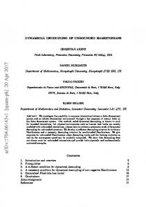
FIG. 1: (a) Spectroscopy of the qubit-TLS system. The qubit and TLS are resonant at f = 7.08 GHz, where the spectrum has an anticrossing with splitting S = 76 MHz. The inset shows the qubit spectrum over a larger range, with the red circle indicating the region of interest. (b) Pulse sequence for probing the qubit-TLS interactions. The π-pulse generates a qubit excitation, which is coherently exchanged back and forth between qubit and TLS during the interaction time τ1 . (c) Coherent oscillations between qubit and TLS, measured using the pulse sequence shown in (b). High switching probability PSW corresponds to the qubit’s ground state |0i, low PSW to the qubit’s excited state |1i. (d-e) Characteristic decay time tdecay and oscillation frequency fosc , extracted from the data in (c). The oscillations decay faster for δΦ 6= 0, a consequence of the increased sensitivity ∂fosc /∂Φ to flux noise.

We use a flux qubit [29], consisting of a superconducting loop interrupted by four Josephson junctions (see

2 Ref. [24] for a detailed description of the device). The qubit’s diabatic states correspond to clockwise and counterclockwise persistent currents ±IP , with IP = 180 nA. The inset of Fig. 1(a) shows a spectrum of the device versus external flux, with Φqb defined as Φqb = Φ+Φ √ 0 /2 and Φ0 = h/2e. The qubit frequency follows fqb = ∆2 + ε2 , where the tunnel coupling ∆ = 5.4 GHz is set by the design parameters and the energy detuning ε = 2IP Φqb /h is controlled by the applied flux. The device is embedded in a SQUID, which is used as a sensitive magnetometer for qubit read-out [18]. At Φqb = Φ∗ = ±4.15 mΦ0 , the qubit becomes resonant with a TLS [30]. The microscopic nature of the TLS is unknown, but studies of two-level systems in similar qubit designs show that the most likely origin is an electric dipole in one of the tunnel junctions [31]. Figure 1(a) shows a magnification of the region around −4.15 mΦ0 , revealing a clear anticrossing with splitting S = 76 MHz. We describe the system using the four states {|0gi, |1gi, |0ei, |1ei}, where (0, 1) are the qubit energy eigenstates and (g, e) refer to the ground and excited state of the TLS. On resonance, |1gi and |0ei are degenerate and coupled by the coupling energy hS. To characterize the coupling, we use the pulse scheme depicted in Fig. 1(b) [32]. Starting with both qubit and TLS in their ground states (|0gi), we rapidly shift the flux to a position δΦ = Φqb − Φ∗ = 1.2 mΦ0 where the qubit frequency fqb = 6.3 GHz is far detuned from the TLS. By applying a microwave pulse, resonant with fqb , we perform a π-rotation on the qubit and put the system in |1gi. We then rapidly shift δΦ to a value close to zero, effectively turning on the interaction S, whereupon the system will oscillate between |1gi and |0ei. After a time τ1 , the interaction is turned off by shifting δΦ away from zero, and we measure the final qubit state by applying a read-out pulse to the SQUID. Since the measurement outcome is stochastic, we repeat the sequence a few thousand times to acquire sufficient statistics to estimate the SQUID switching probability PSW and thereby the qubit state. Figure 1(c) shows the qubit state after the pulse sequence, measured versus interaction time τ1 and flux detuning δΦ. At δΦ = 0 and for τ1 = 1/(2S) = 6 ns, the pulse sequence implements an iSWAP gate between qubit and TLS, taking |0ei → i|1gi and |1gi → i|0ei [32– 34]. The characteristic decay time of the oscillations is shown in Fig. 1(d). The oscillations persist the longest at δΦ = 0; at this point, the decay time is ∼ 800 ns. However, as δΦ is moved away from the optimal point, the decay time quickly decreases to zero. We attribute the reduction in coupling coherence to low-frequency flux noise, present in all superconducting devices [35]. When δΦ 6= 0, fluctuations in δΦ induce variations in the effective coupling frequency fosc [Fig. 1(e)], leading to dephasing of the entangled state. For single qubits, dephasing due to low-frequency fluctuations of the qubit frequency can be reduced in a Hahnecho experiment [21]. By applying a π-pulse after a time

t of dephasing, the qubit’s noise-induced evolution will reverse directions and refocus at time 2t, provided that the fluctuations are slow on the time scale 2t [24, 36]. Here, our goal is to extend such single-qubit refocusing techniques to the mitigation of noise in coupled systems with multiple qubits, which requires implementing refocusing pulses for entangled states. Note that the purpose here is to increase coherence times, as opposed to turning off unwanted couplings [37, 38]. We start by describing the system’s dynamics. Following Refs. [30, 31, 34], we write the total Hamiltonian ˆ =H ˆ qb + H ˆ TLS + H ˆ int , with H ˆ qb = −(h/2)fqb σ as H ˆzqb , TLS ˆ TLS = −(h/2)fTLS σ H ˆz , and with the interactions deqb ˆ int = −(h/2)S σ scribed by H ˆxqb σ ˆxTLS . Here, σ ˆx,z are Pauli TLS operators for the qubit, σ ˆx,z are TLS operators and fTLS is the TLS frequency. To focus on the interactions between the qubit and the TLS, we restrict the discussion to the subspace spanned by the states {|1gi, |0ei}. In the rotating frame of the TLS, the subspace Hamiltonian becomes
ˆ sub = − h δf σ H ˆzsub + S σ ˆxsub , 2

(1)

sub where δf = fTLS − fqb and σ ˆx,z are subspace Pauli operators. The dynamics of Eq. (1) can be visualized on a Bloch sphere, with the north and south poles corresponding to |1gi and |0ei, respectively, and with S and δf representing the length of torque vectors along the xand z-axes [see Fig. 2(b)]. The frequency of the coherent oscillations seen in Fig. 1(c) is then given by the effective coupling strength p (2) fosc = δf 2 + S 2 ,

which is plotted together with the data in Fig. 1(e). With the coupling dynamics described by Eq. (1), we discuss the details of the refocusing sequence, shown in Fig. 2(a-b). The system is brought into the {|1gi, |0ei} subspace by applying a π-pulse to the qubit [step I in Figs. 2(a-b)], followed by a non-adiabatic shift in δΦ to bring the qubit and TLS close to resonance. |1gi is not an eigenstate of the coupled system, so the interaction S will cause the system to rotate around the x-axis, oscillating between |1gi and |0ei. Low-frequency fluctuations in the effective coupling strength will cause the Bloch state vector to fan out (over many realizations of the experiment), and the system loses its phase coherence (step II). The refocusing pulse is now implemented by applying a flux shift pulse that rapidly detunes the qubit and the TLS to δf = 550 MHz. With |δf |  |S|, the state vector is effectively rotating around the z-axis (step III) [19], and we realize a π rotation by setting the pulse duration τrefocus = 0.5/δf . The system is then rapidly brought back into resonance (step IV), and the state vector continues to rotate around the x-axis. The inhomogeneous broadening that caused the state vector to diffuse during the first interval τ1 will now realign them

3 Qubit π-pulse

Flux

I

τ1

0

III

Φrefocus

0

τ2 II IV

(b)

V Time ttotal

f I

II

III

IV

S

z x

Read-out

τrefocus

V S

No refocusing, τ2 = 0, τ1= ttotal Refocusing pulse

4 2 60

S

y

τ1 = 97 ns

τ2 = τ1

6

0

(c)

(d)

8 Time τrefocus [ns]

(a)

80

100 Time τ2 [ns]

120

140

FIG. 3: Calibration of the refocusing pulse, measured by fixing τ1 = 97 ns and looking for the echo signal by sweeping τ2 . The echo appears every time the refocusing pulse generates a rotation by an odd integer of π. The first five refocusing conditions occur at τrefocus = (2n + 1) × 0.5/δf = 0.9, 2.7, 4.5, 6.4, and 8.2 ns, with δf = 550 MHz.

τ1 = 100 ns

decay as [20, 39] τ2 = τ1

Total evolution time ttotal [ns]

FIG. 2: (a) Pulse sequence and (b) Bloch sphere representation of the refocusing protocol. The blue arrows are state vectors, while the red arrows represent the Hamiltonian in Eq. (1). After the qubit π pulse, the system enters the {|1gi, |0ei} subspace (step I). The coupling S rotates the state vector around the x-axis, but due to noise in the effective coupling the state vector fans out (II). The rapid flux pulse Φrefocus generates a large frequency detuning δf , the system will start rotating around the z-axis (III) and eventually complete a π-rotation (IV). The inhomogeneous broadening now refocuses the state vector, giving an echo at V. (c-d) Evolution of the qubit-TLS system, measured with and without a refocusing pulse. A clear echo appears after the refocusing pulse, with a maximum close to τ2 = τ1 . The traces were taken at δΦ = −72 µΦ0 .

again. The refocusing is complete after a time τ2 = τ1 (step V). Figures 2(c-d) illustrate the result of the refocusing sequence. Without the refocusing pulse [Fig. 2(c)], the coherent oscillations between |1gi and |0ei decay almost completely after 100 ns. When inserting a refocusing pulse at τ1 = 100 ns, the oscillations start to revive, eventually forming an echo at τ2 = τ1 . The revival of phase coherence seen in Fig. 2(d) requires careful calibration of the refocusing pulse. Figure 3 shows an example of a calibration experiment, where we fix τ1 = 97 ns and δf = 550 MHz and measure refocused oscillations versus the refocusing time τrefocus . The data shows strong oscillations whenever the refocusing pulse rotates the state vector by an odd integer of π, i.e. when τrefocus = (2n + 1) × 0.5/δf , in agreement with the schematics discussed in Fig. 2(b). We now turn to investigating the decoherence mechanisms and determining the performance of the refocusing protocol. For Gaussian-distributed dephasing noise, we expect the amplitude h(t) of the coherent oscillations to

h(t) = exp[−t/T˜1 ] exp[−(t/Tϕ,N )2 ].

(3)

The exponential decay constant T˜1 is due to energy relaxation, while Tϕ,N represents the dephasing with N refocusing pulses. At δΦ = 0, we measure a pure exponential decay with time constant T˜1 = 800 ns, which is shorter than the relaxation time of both the qubit (T1qb = 10 µs) and the TLS (T1TLS = 1 µs). However, to get an expression for T˜1 , we need to consider all the possible absorption/emission rates in the full four-level system [40]. In the relevant situation hS  kB T  hfTLS , hfqb , we have  1 1 (4) 1/T1qb + 1/T1TLS + (Γ± + Γ∓ ) , 1/T˜1 = 2 2 where Γ± (Γ∓ ) represents relaxation (excitation) be√ tween the two energy eigenstates |±i = (|0gi ± |1ei)/ 2 of Eq. (1), with energy splitting hfosc . The polarization rate Γ± + Γ∓ = S⊥ (fosc )/2 depends on the noise power S⊥ that couples transversely to the diagonalized subspace Hamiltonian in Eq. (1), which for δΦ = 0 corresponds to fluctuations Sδf (fosc ) in the frequency detuning δf [20]. Using Eq. (4) and the measured values of T˜1 , T1qb and T1TLS , we get Sδf (f = 76 MHz) = 2.8 × 106 rad/s. We can not distinguish whether this noise comes from fluctuations in fqb , fTLS or a combination thereof, but we note that the measured value is a few times larger than fluctuations in fqb expected from flux noise. From independent measurements of the flux noise power SΦqb in the same device, we have Sfqb = SΦqb (∂fqb /∂Φqb )2 = 1.1 × 106 rad/s at f = 76 MHz and Φqb = −4.15 mΦ0 [41]. Away from δΦ = 0, the decay envelope becomes Gaussian, and we extract the dephasing time Tϕ,N by fitting the data to Eq. (3), assuming a constant relaxation time T˜1 = 800 ns. The extracted decay times versus flux δΦ are shown in Fig. 4(a). The refocusing sequence gives considerably longer decay times over the full range of the measurement except around δΦ = 0, where the decay is

4

600

0 0

400

t [ns]

700

200

PSW

(c)

0

N=1 N=0

-100 -50 Flux detuning

1/e decay time [ns]

(b)

1 h

1/e decay time [ns]

(a)800

600 400 200

0

0

0 1 2 3 4 5 6 7 8 # of refocusing pulses N

No refocusing (N=0)

0.8 0.6 0.4

PSW

(d)

Refocusing pulses

0.8 0.6 0.4 0

100

200

300 400 Time [ns]

500

600

700

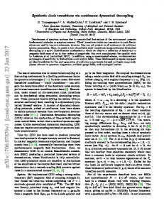
FIG. 4: (a) Decay times of the coherent oscillations, measured with (N =1) and without (N =0) a refocusing pulse. At δΦ = 0, the decay is limited by energy relaxation, but the coherence times decrease away from δΦ = 0 due to increased sensitivity to flux noise. For large |δΦ|, the refocusing sequence improves the decay time by more than a factor of four. The inset show examples of decay envelope h(t), measured at δΦ = −60 µΦ0 . For the N =1 case, we use τ1 = τ2 = t/2. (b) Decay times of multi-pulse refocusing sequences, showing the improvement coherence as the number of pulses increases. (c-d) Time evolution of the qubit-TLS system, measured with and without refocusing pulses. Note the echo signals appearing after each refocusing pulse, giving a strong enhancement of the coherence time. The data is taken at δΦ = −84 µΦ0 .

limited by T˜1 . Note that to capture both the exponential and the Gaussian decay, we plot the time Te for the envelope to decrease by a factor 1/e. Examples of decay envelopes together with fits are shown in the inset of Fig. 4(a), measured with and without a refocusing pulse at δΦ = −60 µΦ0 . We model the decreased phase coherence away from δΦ = 0 in terms of flux noise. In analogy with coherence measurements on single flux qubits [42], we assume 1/f -type fluctuations in Φ, with noise spectrum SΦ (ω) = AΦ /|ω|. The flux noise couples to the oscillation frequency fosc through Eq. (2), leading to the dephasing rate p 1/Tϕ,N = 2π cN AΦ ∂fosc /∂Φ . (5) Here, cN =0 = ln(1/ωlow t) and cN =1 = ln(2) relate to the filtering properties of the pulse sequence [20, 24], with the low-frequency cut-off ωlow /2π = 1 Hz fixed by the measurement protocol. The solid lines in Fig. 4(a) are fits to

Eq. (5), using a single fitting parameter AΦ = (1.4 µΦ0 )2 . This amount of flux noise is consistent with previous results [24, 42]. The overall good agreement between Eq. (5) and the data verifies the noise model and further confirms the validity of the refocusing sequence. However, for the range δΦ > −30 µΦ0 , the refocused data shows slightly lower coherence times than expected from the model. We attribute this to the finite rise time of our shift pulses. The refocusing sequence requires the frequency sweep rate ∂f /∂t to be fast compared to the interaction timescale 1/S ∼ 10 ns (to make the shifts non-adiabatic), but slow compared to the qubit precession time 1/fqb ∼ 0.2 ns (to avoid driving the system out of the {|1gi, |0ei} subspace). The constraints can be phrased in terms of the probability of undergoing Landau-Zener transitions, giv2 ing S 2  ∂f /∂t  fqb [43]. Using pulses with 1.5 ns Gaussian rise time, we have ∂f /∂t ≈ 550 MHz/1.5 ns = (606 MHz)2 , and on average the constraints are well fulfilled. However, ∂f /∂t is lower during the slowest parts of the shift pulse (the beginning and the end), and artifacts due to imperfect non-adiabaticity appear when these parts of the pulse occur where the effective coupling is the strongest (at δΦ = 0). The limited nonadiabaticity is also the reason for the slight asymmetry around δΦ = 0 in Fig. 1(c) [22]. We now extend the refocusing technique to implement dynamical decoupling protocols with multi-pulse sequences. For 1/f -type noise, it has been shown that the Carr-Purcell sequence [23], consisting of equally spaced π-rotations, improves coherence times by filtering the noise at low frequencies [24, 36, 44, 45]. Figures 4(cd) show the coherent evolution of the system when repeatedly applying refocusing pulses. Echo signals form between each pair of π pulses, giving considerable longer coherence times compared to the N = 0 case. The increase in decay time with the number of refocusing pulses N is plotted in Fig. 4(b), measured for a few different values of δΦ. The improvement is consistent with the filtering properties of the pulse sequence; for larger N , the filter cut-off frequency increases and, since the noise is of 1/f -type, the total noise power leading to dephasing is reduced. To summarize, we have implemented refocusing and dynamical decoupling techniques to correct for noise and improve the lifetime of entangled two-level systems. Although implemented between a flux qubit and a microscopic two-level system, the method applies to any transversely coupled spin-1/2 systems where the relative frequency detuning can be controlled. We expect the findings to be of importance when developing decoupling techniques to improve two-qubit gate fidelities. We thank K. Harrabi for assistance with device fabrication and O. Zwier, X. Jin and E. Paladino for helpful discussions. This work was supported by NICT.

5

[1] M. J. Bremner, C. M. Dawson, J. L. Dodd, A. Gilchrist, A. W. Harrow, D. Mortimer, M. A. Nielsen, and T. J. Osborne, Phys. Rev. Lett. 89, 247902 (2002). [2] E. Lucero, M. Hofheinz, M. Ansmann, R. C. Bialczak, N. Katz, M. Neeley, A. D. O’Connell, H. Wang, A. N. Cleland, and J. M. Martinis, Phys. Rev. Lett. 100, 247001 (2008). [3] J. Chow, L. DiCarlo, J. Gambetta, F. Motzoi, L. Frunzio, S. Girvin, and R. Schoelkopf, Phys. Rev. A 82, 040305 (2010). [4] E. Knill, D. Leibfried, R. Reichle, J. Britton, R. B. Blakestad, J. D. Jost, C. Langer, R. Ozeri, S. Seidelin, and D. J. Wineland, Phys. Rev. A 77, 012307 (2008). [5] R. C. Bialczak, M. Ansmann, M. Hofheinz, E. Lucero, M. Neeley, A. D. O’Connell, D. Sank, H. Wang, J. Wenner, M. Steffen, et al., Nat Phys 6, 409 (2010). [6] J. Chow, A. C´ orcoles, J. Gambetta, C. Rigetti, B. Johnson, J. Smolin, J. Rozen, G. Keefe, M. Rothwell, M. Ketchen, et al., Phys. Rev. Lett. 107, 080502 (2011). [7] A. Dewes, F. R. Ong, V. Schmitt, R. Lauro, N. Boulant, P. Bertet, D. Vion, and D. Esteve, Phys. Rev. Lett. 108, 057002 (2012). [8] M. Steffen, M. Ansmann, R. C. Bialczak, N. Katz, E. Lucero, R. McDermott, M. Neeley, E. M. Weig, A. N. Cleland, and J. M. Martinis, Science 313, 1423 (2006). [9] T. Yamamoto, Y. A. Pashkin, O. Astafiev, Y. Nakamura, and J. S. Tsai, Nature 425, 941 (2003). [10] T. Hime, P. A. Reichardt, B. L. T. Plourde, T. L. Robertson, C.-E. Wu, A. V. Ustinov, and J. Clarke, Science 314, 1427 (2006). [11] R. C. Bialczak, M. Ansmann, M. Hofheinz, M. Lenander, E. Lucero, M. Neeley, A. D. O’Connell, D. Sank, H. Wang, M. Weides, et al., Phys. Rev. Lett. 106, 060501 (2011). [12] J. Majer, J. M. Chow, J. M. Gambetta, J. Koch, B. R. Johnson, J. A. Schreier, L. Frunzio, D. I. Schuster, A. A. Houck, A. Wallraff, et al., Nature 449, 443 (2007). [13] M. A. Sillanp¨ a¨ a, J. I. Park, and R. W. Simmonds, Nature 449, 438 (2007). [14] A. O. Niskanen, K. Harrabi, F. Yoshihara, Y. Nakamura, S. Lloyd, and J. S. Tsai, Science 316, 723 (2007). [15] J. H. Plantenberg, P. C. de Groot, C. J. P. M. Harmans, and J. E. Mooij, Nature 447, 836 (2007). [16] C. Rigetti and M. Devoret, Phys. Rev. B 81, 134507 (2010). [17] P. C. de Groot, J. Lisenfeld, R. N. Schouten, S. Ashhab, A. Lupa¸scu, C. J. P. M. Harmans, and J. E. Mooij, Nat Phys 6, 763 (2010). [18] I. Chiorescu, Y. Nakamura, C. J. P. M. Harmans, and J. E. Mooij, Science 299, 1869 (2003). [19] J. R. Petta, A. C. Johnson, J. M. Taylor, E. A. Laird, A. Yacoby, M. D. Lukin, C. M. Marcus, M. P. Hanson, and A. C. Gossard, Science 309, 2180 (2005). [20] G. Ithier, E. Collin, P. Joyez, P. Meeson, D. Vion, D. Esteve, F. Chiarello, A. Shnirman, Y. Makhlin, and

J. Schriefl, Phys. Rev. B 72, 134519 (2005). [21] E. Hahn, Phys. Rev. 80, 580 (1950). [22] M. Hofheinz, H. Wang, M. Ansmann, R. C. Bialczak, E. Lucero, M. Neeley, A. D. O’Connell, D. Sank, J. Wenner, J. M. Martinis, et al., Nature 459, 546 (2009). [23] H. Carr and E. Purcell, Phys. Rev. 94, 630 (1954). [24] J. Bylander, S. Gustavsson, F. Yan, F. Yoshihara, K. Harrabi, G. Fitch, D. G. Cory, Y. Nakamura, J.-S. Tsai, and W. D. Oliver, Nat Phys 7, 565 (2011). [25] L. Viola, E. Knill, and S. Lloyd, Phys. Rev. Lett. 82, 2417 (1999). [26] H. Cummins, G. Llewellyn, and J. Jones, Phys. Rev. A 67, 042308 (2003). [27] A. J. Kerman and W. D. Oliver, Phys. Rev. Lett. 101, 070501 (2008). [28] N. Khaneja, F. Kramer, and S. J. Glaser, Journal of Magnetic Resonance 173, 116 (2005). [29] J. Mooij, T. Orlando, L. Levitov, L. Tian, van der Wal CH, and S. Lloyd, Science 285, 1036 (1999). [30] R. W. Simmonds, K. M. Lang, D. A. Hite, S. Nam, D. P. Pappas, and J. M. Martinis, Phys. Rev. Lett. 93, 077003 (2004). [31] A. Lupa¸scu, P. Bertet, E. F. C. Driessen, C. J. P. M. Harmans, and J. E. Mooij, Phys. Rev. B 80, 172506 (2009). [32] M. Neeley, M. Ansmann, R. C. Bialczak, M. Hofheinz, N. Katz, E. Lucero, A. O’Connell, H. Wang, A. N. Cleland, and J. M. Martinis, Nat Phys 4, 523 (2008). [33] N. Schuch and J. Siewert, Phys. Rev. A 67, 032301 (2003). [34] A. M. Zagoskin, S. Ashhab, J. R. Johansson, and F. Nori, Phys. Rev. Lett. 97, 077001 (2006). [35] F. Wellstood, C. Urbina, and J. Clarke, Appl. Phys. Lett. (1987). [36] M. J. Biercuk, H. Uys, A. P. VanDevender, N. Shiga, W. M. Itano, and J. J. Bollinger, Nature 458, 996 (2009). [37] D. Leung, I. Chuang, F. Yamaguchi, and Y. Yamamoto, Phys. Rev. A 61, 042310 (2000). [38] L. M. Vandersypen, M. Steffen, G. Breyta, C. S. Yannoni, M. H. Sherwood, and I. L. Chuang, Nature 414, 883 (2001). [39] G. Falci, A. D’arrigo, A. Mastellone, and E. Paladino, Phys. Rev. Lett. 94, 167002 (2005). [40] E. Paladino, A. Mastellone, A. D’arrigo, and G. Falci, Phys. Rev. B 81, 052502 (2010). [41] F. Y. et. al, in preparation (2012). [42] F. Yoshihara, K. Harrabi, A. O. Niskanen, Y. Nakamura, and J. S. Tsai, Phys. Rev. Lett. 97, 167001 (2006). [43] D. M. Berns, M. S. Rudner, S. O. Valenzuela, K. K. Berggren, W. D. Oliver, L. S. Levitov, and T. P. Orlando, Nature 455, 51 (2008). [44] L. Faoro and L. Viola, Phys. Rev. Lett. 92, 117905 (2004). [45] G. Falci, A. D’Arrigo, A. Mastellone, and E. Paladino, Phys. Rev. A 70, 040101 (2004).