Optimally combining dynamical decoupling and quantum error

Optimally combining dynamical decoupling and quantum error correction Gerardo A. Paz-Silva(1,4) and D. A. Lidar(1,2,3,4) Departments of (1) Chemistry, (2) Physics, and (3) Electrical Engineering, and (4) Center for Quantum Information Science & Technology, University of Southern California, Los Angeles, California 90089, USA

arXiv:1206.3606v1 [quant-ph] 15 Jun 2012

We show how dynamical decoupling (DD) and quantum error correction (QEC) can be optimally combined in the setting of fault tolerant quantum computing. To this end we identify the optimal generator set of DD sequences designed to protect quantum information encoded into stabilizer subspace or subsystem codes. This generator set, comprising the stabilizers and logical operators of the code, minimizes a natural cost function associated with the length of DD sequences. We prove that with the optimal generator set the restrictive localbath assumption used in earlier work on hybrid DD-QEC schemes, can be significantly relaxed, thus bringing hybrid DD-QEC schemes, and their potentially considerable advantages, closer to realization.

Introduction.—The nemesis of quantum information processing is decoherence, the outcome of the inevitable interaction of a quantum system with its environment, or bath. Several methods exist that are capable of mitigating this undesired effect. Of particular interest to us here are quantum error correction (QEC) [1–4] and dynamical decoupling (DD) [5–9]. QEC is a closed-loop control scheme which encodes information and flushes entropy from the system via a continual supply of fresh ancilla qubits, which carry off error syndromes. DD is an open-loop control scheme that reduces the rate of entropy growth by means of pulses applied to the system, which stroboscopically decouple it from the environment. QEC and DD have complementary strengths and weaknesses. QEC is relatively resource-heavy, but can be extended into a fully fault-tolerant scheme, complete with an accuracy threshold theorem [10–15]. DD demands significantly more modest resources, can theoretically achieve arbitrarily high decoherence suppression [16–23], but cannot by itself be made fully faulttolerant [24]. A natural question is whether a hybrid QEC-DD scheme is advantageous relative to using each method separately in the setting of fault-tolerant quantum computing (FTQC). Typically, improvements in gate accuracy achieved by DD mean that more noise can be tolerated by a hybrid QEC-DD scheme than by QEC alone, and that invoking DD can reduce the overhead cost of QEC. While early studies identified various advantages [25–27], they did not address fault tolerance. A substantial step forward was taken in Ref. [28], which analyzed “DD-protected gates” (DDPGs) in the FTQC setting. Such gates are obtained by preceding every physical gate (i.e., a gate acting directly on the physical qubits) in a fault tolerant quantum circuit by a DD sequence. DDPGs can be less noisy than the bare, unprotected gates, since DD sequences can substantially reduce the strength of the effective systemenvironment interaction just at the moment before the physical gate is applied. The gains can be very substantial if the intrinsic noise per gate is sufficiently small, and can make quantum computing scalable with DDPGs, where it was not with unprotected gates [28]. The analysis in Ref. [28] assumed a “local” perspective. Rather than analyzing the complete FT quantum circuit, each single- or multi-qubit gate was separately DD-protected. This

required a strong locality constraint limiting the spatial correlations in the noise, known as the “local bath” assumption. Unfortunately, many physically relevant error models violate this assumption [13–15]. Here we aim to integrate DD with FTQC using a global perspective. This appears to be necessary in order to achieve high order decoupling in a multi-qubit setting, under general noise models. Rather than protecting individual gates we shall show how an entire FT quantum register, including data and ancilla qubits, can be enhanced using DD. This will allow us to relax the restrictive local bath assumption. Along the way, we identify a DD strategy that takes into account the basic structure and building blocks of FT quantum circuits, and identify optimal DD pulse sequences compatible with this structure, that drastically reduce the number of pulses required compared with previous designs. Such a reduction is crucial in order to reap the benefits of DD protection, for if a DD sequence becomes too long, noise can accumulate to such an extent as to outweigh any DD enhancements. The noise model.—We assume a completely general noise Hamiltonian H acting on the joint system-bath Hilbert space, the only assumption being that kHk < ∞, where k · k denotes the sup-operator norm (the largest singular value, or largest eigenvalue for positive operators) [29]. Informally, H contains a “good” and a “bad” part, the latter being the one we wish to decouple. H is k-local, i.e., involves up to k-body interactions, with k ≥ 1. We allow for arbitrary interactions between the system and the bath, as well as between different parts of the system or between different parts of the bath. See Fig. 1. Dynamical decoupling.—DD pulse sequences comprise a series of rapid unitary rotations of the system qubits about different axes, separated by certain pulse intervals, and generated by a control Hamiltonian HC (t). They are designed to suppress decoherence arising from the “bad” terms in H. This is typically manifested in the suppression or even vanishing of the first N orders, in powers of the total evolution time T , of the time-dependent perturbation expansion (Dyson or Magnus series [30]) of the evolution operator RT U (T ) = T exp(−i 0 H(t)dt), where H(t) is H in the “toggling frame” (the interaction picture generated by the DD

2 out to be too strong for our purposes. Note that any operator A can decomposed as A = A0 +Ar , where A0 (Ar ) denotes the component that commutes (does not commute) with all elements of a MOOS, i.e., A0 ∈ CΩ . ˆ lasting We shall say that a pulse sequence with generator set Ω ˆ total time T achieves “N th order Ω-decoupling” if the joint system-bath unitary evolution operator at the conclusion of the sequence becomes U [N ] (T ) = eiT H

eff,N

(T )

,

(1)

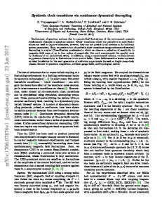
where the effective Hamiltonian is FIG. 1. Qubits and corresponding baths represented as white and black circles respectively. Bath operators corresponding to different operators inside a box do not necessarily commute, while they do if the baths are in different boxes. The Hamiltonians considered are general within each box, but not between them. In (a) a diagram of the “local bath assumption” used in Ref. [28] is shown, while (b) represents the general scenario considered in fault-tolerance [13–15]. In (c) we illustrate one of our key results: domains are allowed to grow logarithmically in the size of the problem the FTQC is solving. The dark grey boxes represent such domains, each containing O[log(ktot )] physical qubits at the highest level of concatenation, where ktot is the total number of logical qubits. When two domains need to interact (light grey box), then the joint DD generator set is used and the locality of the bath is updated accordingly.

pulse sequence Hamiltonian HC (t)) [8], and T denotes timeordering. When the first non-identity system-term of U (T ) appears at O(T N +1 ) one speaks of N th order decoupling. Such DD sequences are now known and well understood [31]. Most DD sequences can be defined in terms of pulses chosen from a mutually orthogonal operator set (MOOS), i.e., a |Ω| set of unitary and Hermitian operators Ω = {Ωi }i=1 , Ω2i = 11 (identity) ∀i, and such that any pair of operators either commute or anticommute [21]. The generator set of a MOOS ˆ ˆ = {Ωi }|Ω| (gMOOS), Ω i=1 , is defined as the minimal subset ˆ ⊆ Ω such that every element of Ω is a product of elements Ω ˆ but no element in Ω ˆ is itself a product of elements in Ω ˆ of Ω [32]. All deterministic DD sequences are finitely generated, meaning that the pulses are elements, or products of elements, of a finite DD generator set (DDGS), which we identify with ˆ the gMOOS Ω. The centralizer of the MOOS Ω is CΩ := {A | [A, Ω] = 0}, i.e., the set of operators which commute with all MOOS elements. A good example of a gMOOS is the generator set Pˆn = {X (i) , Z (i) }ni=1 , where X (i) (Z (i) ) denotes the Pauli-x (z) matrix acting on the ith qubit, of the Pauli group Pn = P1⊗n on n qubits (the group of all n-fold tensor products of the standard Pauli matrices P1 = {11, X, Y, Z}, modulo Z2 ). For simplicity, since we will be dealing with qubits and are particularly interested in decoupling sequences that allow for ˆ ⊆ Pn . It bitwise pulses, we shall assume henceforth that Ω is necessary to recast the notion of decoupling order in the MOOS scenario, since the previously mentioned notion turns

H eff,N (T ) ≡ H0eff,N (T ) + Hreff,N (T ) T kHreff,N (T )k H0eff,N (T )

N +1

∼ O[(T kHk) ∈ CΩ .

]

(2a) (2b) (2c)

The subspace invariant under CΩ has therefore been decoupled, in the sense that terms not commuting with CΩ appear only in O(T N +1 ). Thus the choice of the pulse generator set ˆ determines what subspace(s) can be decoupled, and conΩ versely a subspace one is interested in decoupling to arbitrary ˆ order implies a choice of Ω. Optimization of the DDGS.—We define the cost of a DD sequence as the total number of pulse intervals it uses to achieve ˆ N th order Ω-decoupling. For all known DD sequences (even those optimized for multiple qubits [33]), the cost is at least ˆ

|Ω| cΩ , ˆ = f (N )

(3)

and f (N ) depends on the particular DD sequence. Pulse interval optimization has already reduced f (N ) from 2N for CDD to N + 1 for NUDD [31]. Here we are concerned instead with ˆ to which end the the optimization of the cost exponent |Ω|, following theorem will prove to be crucial (for the proof see [34]) [35]: Theorem 1 Let B be a subgroup of the the Pauli group Pn , ˆ ⊆ Pn which decouˆ Consider a DDGS Ω generated by B. ples B in the sense that the only element in the intersection ˆ B|. ˆ Moreover, the DDGS between CΩ and B is 11. Then |Ω|≥| ˆ =B ˆ decouples B in the desired sense, and automatically Ω saturates the bound. As an immediate application, we reproduce the well-known ˆ = Pˆn , and hence |Ω| ˆ = 2n, is optimal for n result that Ω qubits without encoding [8]. Indeed, in this case the most general noise Hamiltonian is spanned by the elements of the ˆ = 2n and thus by Theorem 1 “error group” B = Pn , so |B| ˆ it must be that |Ω| ˆ ≥ 2n. On the other for any DDGS Ω ˆ ˆ hand Ω = Pn indeed decouples Pn since CΩ = 11. Note also that Eq. (2c) yields H0eff,N (T ) ∝ 11. Moreover, since DD ˆ sequences are known that achieve N th order Ω-decoupling for n ≥ 1 qubits (specifically CDD [16] and NUDD [21], with explicit Pˆn -based constructions given in Ref. [21]), the generating set Pˆn is the smallest one capable of achieving N th order decoupling of a general n-qubit Hamiltonian. However,

3 as we discuss next, there is a better choice for the purpose of protecting a code subspace. DD generator set for a QEC code.—Consider a set of n physical qubits encoding k logical and r gauge qubits via some distance d code, i.e., an [[n, k, r, d]] subsystem code [36–38] (or an [[n, k, d]] stabilizer code [4] for r = 0), subject to the general noise model described above. Let ˆ = {Sµ }Q denote the stabilizer generators, where Q = S µ=1 ˆ = {X (i) , Z (i) }k denote the logicaln − (k + r), let L L L i=1 ˆ = {Xν , Zν }r the operator generators of the code, and G ν=1 gauge operator generators. In the [[n, k, d]] code case, each error correctable by the code maps a codeword to an syndrome subspace labeled by an error syndrome, i.e., a sequence of ±1 eigenvalues of the stabilizer generators [4]. In order to properly integrate DD with QEC, we require a set of DD genˆ which preserves the error syndromes to order N , erators Ω i.e., such that H0eff,N acts trivially on each of the syndrome subspaces and does not mix them, so that at the conclusion of the sequence the original noise model for which the code was chosen, is preserved (again, to order N ). This form of the N th ˆ order Ω-decoupling requirement will enable error correction to function as intended. A key observation is that in light of this, we do not need to protect the complete 2n -dimensional Hilbert space H, but rather the 2n−k syndrome subspaces. To this end we propose to choose a complete set of stabilizer and logical operator generators as DD sequence generaˆ =S ˆ∪L ˆ [39]. We refer to any DD sequence tors, i.e., let Ω having a DDGS of this type as an “SLDD” sequence. With ˆ ⊂ Ω. ˆ Now note that if CˆΩ ⊆ Ω, then this choice, CˆΩ = S ˆ ˆ the elements in CΩ commute and they define |CΩ | = 2|CΩ | subspaces characterized by their eigenvalue under the action ˆ of CˆΩ . In this case we have independent N th order Ωeff,N decoupling of each of these subspaces. In other words, H0 leaves each of the syndrome subspaces invariant and does not ˆ =S ˆ∪L ˆ also mix them, as desired. Note that the choice Ω applies to subsystem codes [36–38]. In this case each of the syndrome subspaces can be decomposed as Hlogical ⊗ Hgauge , ˆ ∪G ˆ = C ˆ , since the gauge where Hlogical is invariant under S Ω operators act non-trivially on Hgauge only. Before proving its optimality, we next compare the cost of the SLDD sequence to decoupling the entire Hilbert space. Relative cost of SLDD.—For an [[n, k, d]] code and an SLDD sequence, the number of stabilizer generators (n − k) ˆ = n + k, plus logical operator generators (2k) yields |Ω| n+k which means that cS∪ = f (N ) < c = f (N )2n . Ofˆ L ˆ Pˆn √ cPˆn . In the case of [[n, k, r, d]] ten n k, so that cS∪ ˆ L ˆ ∼ subsystem codes [38] the advantage is more pronounced: the ˆ = n+k−r. As an exnumber of stabilizers is n−k−r, so |Ω| ample consider the Bacon-Shor [[m × m, 1, (m − 1)2 , 3]] subsystem code [36], which has the highest (analytically) known fault-tolerant threshold for error correction routines with [13] and without measurements [40]. In this case one would have 2m cS∪ = (cPˆ 2 )1/m , a polynomial advantage that ˆ L ˆ = f (N ) m grows with the block size m. Choice of DDGS for protecting ancilla states.—The protec-

tion of certain ancilla states is also an important part of fault tolerance. Such states can be thought of as QEC codes with √ small stabilizer sets. E.g., |catm,+ i = (|0i⊗a + |1i⊗a )/ 2 is often used for fault-tolerant stabilizer measurements or for teleportation of encoded information. The stabilizer is generated by {X ⊗a , {Zi Zi+1 }a−1 i=1 }, and equals the DDGS. Decoupling multiple subspaces or subsystems.—How should one choose an optimal DDGS to decouple different subspaces simultaneously? Assume that there are distinct and non-overlapping sets of {ni } physical qubits comprising a quantum register, e.g., a complete register comprising k logical qubits, along with the corresponding ancillas. Assume p that they Pp are partitioned into sets of sizes {ki }i=1 , such that k = i=1 ki , and that each set i is encoded in some subsystem (or subspace) code [[ni , ki , ri , di ]]. For each block of ki logical qubits we have an SLDD sequence with DDGS î = S î ∪ L ˆ i . Let the Hamiltonians of the different sets be Ω {Hi }, and spanned by the error groups {Bi ⊂ Pni }. Using ˆ i is optimal for error group Theorem 1, it follows that if Ω ˆ tot = ∪i Ω ˆ B optimally decouples the joint HamilBi then Ω i tonian spanned by ∪i Bi . This form of composing a larger DDGS out of smaller modules guarantees that each term of a general Hamiltonian acting on the whole register must anˆ tot , which in turn ticommute with at least one element in Ω ˆ implies that Ωtot , used to construct, e.g., a CDD or NUDD seˆ tot -decoupling quence, is capable of independent N th order Ω of each subspace or subsystem. Optimal DDGS for concatenated QEC codes.—Many FTQC constructions are based on concatenated QEC codes [41], so what is the optimal DDGS for this case, cost-wise? Suppose an [[n, k, r, d]] code is concatenated R times. A complete generator set for all the stabilizers of such a code ˆ (q) , where S ˆ (q) is the stabilizer generator is given by ∪R q=1 S ˆ (R) denote the set of Rthset of concatenation level q. Let L concatenation level logical generators. Theorem 2 The optimal DDGS for decoupling all the syndrome subspaces at concatenation level R is the SLDD set ˆ = ∪R S ˆ (q) ∪ L ˆ (R) , where |Ω| ˆ = nR − (k + r)R + 2k R . Ω q=1 Note that there are alternatives to this “top-level” SLDD strategy; e.g., one could concatenate the DDGS for each block at each level q, but this would result in exponentially more DD pulses. Note also that by setting R = 1 Theorem 2 reduces to the optimality of SLDD for subspace or subsystem codes, ˆ = n + k − r as claimed above. The subspace case is with |Ω| recovered by setting r = 0. Proof. The number of physical qubits after R levels of concatenation of any [[n, k, r, d]] subsystem stabilizer code is n(R) = nR , and the error group for the entire Hilbert space is the Pauli group Pn(R) . We need to protect the 2Q(R) synˆ (q) | is the total drome subspaces, where Q(R) = | ∪R q=1 S number of stabilizer generators after the code is concatenated R times. Q(R) = n(R) − L(R) − G(R), where L(R) = k R [G(R)] is the number of logical (gauge) qubits at level R, and L(R) + G(R) = (k + r)R [42].

4 ˆ = ∪R S ˆ (q) ∪ The SLDD sequence generated by Ω q=1 ˆ (R) satisfies the requirement of independent N th order Ωˆ L Q(R) decoupling of the 2 syndrome subspaces since the stabilizers (as DD pulses) remove the errors at each level q, logical included (recall that a logical error at level q −1 anticommutes with at least one level q stabilizer generator), but not the logˆ (R) as DD ical errors at the top level, for which we need L ˆ pulses. Moreover, for this sequence |Ω| = Q(R) + 2L(R) = nR − (k + r)R + 2k R as claimed. Thus what remains is to prove its optimality. Any operator in Pn(R) which is not a stabilizer or gauge operator acts as an error either within or between syndrome subspaces. Thus our choice of code dictates which elements of Pn(R) act as errors, and clearly this error set is precisely B = Pn(R) /CΩ , where the centralizer generator is CˆΩ = ˆ (q) ∪ G ˆ (q) . We have |CˆΩ | = Q(R) + 2G(R). On the ∪R q=1 S ˆ other hand |B| = 2n(R) − |CˆΩ | = Q(R) + 2L(R), so that ˆ and B ∩ CΩ = 11, which proves the optimality of ˆ = |Ω| |B| ˆ |Ω| by virtue of Theorem 1. Optimizing the choice of DDGS for a complete quantum register: beyond the local bath assumption.—We have now assembled and described all the ingredients for optimally combining DD with FTQC for protection of a complete quantum register. However, we must ensure that the cost of implementing the DD sequence does not spoil quantum speedups. To this end we consider once more an [[n, k, r, d]] subsystem code concatenated R times, used to encode an entire quantum register, and divide the register into d(R) domains (e.g., a code block along with ancillas) of size kD (R) = O(k R ) logical qubits, such that the total number of logical qubits in the register is ktot = d(R)kD (R). We then optimally decouple the ith domain using an SLDD sequence generated by ˆ i = ∪R S ˆ (q) ∪ L ˆ (R) , i ∈ {1, . . . d(R)} (where S ˆ (q) and Ω q=1 i i i (R) ˆ L act non-trivially only on the qubits in the domain i), and i ask for the maximal allowed size of each domain such that the DD sequence cost scales polynomially in ktot , as this will ensure that any exponential quantum speedup is retained. Corollary 1 In a fault tolerant quantum computation the maximal allowed domain size compatible with a DDGS havˆ |Ω| ing cost cΩ = poly(ktot ), is O[log(ktot )]. ˆ = f (N ) Proof. We assume that the total cost per domain cΩ ˆ is Eq. (3) as it captures all known DD sequences. Theorem 2 shows ˆ = O[nR − (k + r)R + 2k R ] (the O symbol is that |Ω| used since we allow for the presence of ancillas in the domain). We may assume that the code has parameters such that ˆ = O(k R ) = O[kD (R)]. Now recall n ∼ r ∼ k, so that |Ω| that R = O[log log(ktot )] in a fault-tolerant simulation of a ˆ |Ω| quantum circuit [43]. Therefore cΩ = poly(ktot ) ˆ = f (N ) requires kD (R) = O[log(poly(ktot ))] = O[log(ktot )]. Corollary 1 means that we can relax the local bath assumption, an assumption tantamount to assuming constant domain size kD ≤ 2 [28]; instead we find that domains are allowed to grow logarithmically with problem size. When two do-

ˆ i ∪Ω ˆj mains i and j are required to interact, the joint DDGS Ω should be used [see Fig. 1(c)]. If the result is that at the highest concatenation level the noise per gate has been reduced (as shown explicitly for the local bath setting in Ref. [28]), then a reduction in the number of required concatenation levels is enabled, hence reducing the overall overhead, or the effective noise threshold. Enhanced fidelity gates via DD.—So far we discussed the problem of protecting stored quantum information; what about computation? Quantum logic operations can be combined with DD, e.g., using “decouple while compute” schemes [44, 45], or (concatenated) dynamically corrected gates [(C)DCGs] for finite-width pulses [46], or dynamically protected gates [28] in the zero-width (ideal) pulse limit. The optimal SLDD scheme introduced here is directly portable into the latter two schemes, since they use the same DD building blocks and the associated group structure. It is important to emphasize that SLDD sequences require only bitwise (i.e., transversal) pulses, and can be generated by one-local Hamiltonians, thus not altering the assumptions of the CDCG construction. More importantly, the polynomial scaling guaranteed by Corollary 1 also applies in the quantum logic scenario, thus allowing, in principle, a fidelity improvement without sacrificing the speedup of quantum computing. Conclusions and outlook.—All known DD sequences scale exponentially with the cardinality of their generating sets [Eq. (3)]. In this work we identified the optimal generating set in the general context of protection of encoded information. This allowed us to show how DD and FTQC can be optimally integrated. In doing so we relaxed the local-bath assumption and showed that it can be replaced with domains growing logarithmically with problem size. Two important open problems remain: to demonstrate that DD-enhanced FTQC results in improved resource overheads and lower noise thresholds, and to identify, or rule out, multi-qubit DD sequences with subexponential scaling in the the cardinality of their generating sets. Acknowledgments.—Supported by the US Department of Defense and the Intelligence Advanced Research Projects Activity (IARPA) via Department of Interior National Business Center contract number D11PC20165. The U.S. Government is authorized to reproduce and distribute reprints for Governmental purposes notwithstanding any copyright annotation thereon. The views and conclusions contained herein are those of the authors and should not be interpreted as necessarily representing the official policies or endorsements, either expressed or implied, of IARPA, DoI/NBC, or the U.S. Government.

[1] [2] [3] [4] [5]

P. Shor, Phys. Rev. A, 52, R2493 (1995). A. Calderbank and P. Shor, Phys. Rev. A, 54, 1098 (1996). A. Steane, Proc. R. Soc. London Ser. A, 452, 2551 (1996). D. Gottesman, Phys. Rev. A, 54, 1862 (1996). L. Viola and S. Lloyd, Phys. Rev. A, 58, 2733 (1998).

5 [6] P. Zanardi, Phys. Lett. A, 258, 77 (1999). [7] L.-M. Duan and G. Guo, Phys. Lett. A, 261, 139 (1999). [8] L. Viola, E. Knill, and S. Lloyd, Phys. Rev. Lett., 82, 2417 (1999). [9] For a recent review see W. Yang, Z.-Y. Wang, and R.-B. Liu, Front. Phys., 6, 2 (2011). [10] D. Aharonov and M. Ben-Or, SIAM J. Comput., 38, 1207 (2008). [11] E. Knill, R. Laflamme, and W. Zurek, Proc. R. Soc. London Ser. A, 454, 365 (1998). [12] B. Terhal and G. Burkard, Phys. Rev. A, 71, 012336 (2005). [13] P. Aliferis, D. Gottesman, and J. Preskill, Quantum Inf. Comput., 6, 97 (2006). [14] D. Aharonov, A. Kitaev, and J. Preskill, Phys. Rev. Lett., 96, 050504 (2006). [15] H. K. Ng and J. Preskill, Phys. Rev. A, 79, 032318 (2009). [16] K. Khodjasteh and D. A. Lidar, Phys. Rev. Lett., 95, 180501 (2005). [17] G. Uhrig, Phys. Rev. Lett., 98, 100504 (2007). [18] W. Yang and R.-B. Liu, Phys. Rev. Lett., 101, 180403 (2008). [19] G. S. Uhrig, Phys. Rev. Lett., 102, 120502 (2009). [20] J. R. West, B. H. Fong, and D. A. Lidar, Phys. Rev. Lett., 104, 130501 (2010). [21] Z.-Y. Wang and R.-B. Liu, Phys. Rev. A, 83, 022306 (2011). [22] W.-J. Kuo and D. A. Lidar, Phys. Rev. A, 84, 042329 (2011). [23] L. Jiang and A. Imambekov, Phys. Rev. A, 84, 060302 (2011). [24] K. Khodjasteh, T. Erdélyi, and L. Viola, Phys. Rev. A, 83, 020305 (2011). [25] M. S. Byrd and D. A. Lidar, Phys. Rev. Lett., 89, 047901 (2002). [26] N. Boulant, M.A. Pravia, E.M. Fortunato, T.F. Havel and D.G. Cory, Quant. Inf. Proc., 1, 135 (2002). [27] K. Khodjasteh and D. A. Lidar, Phys. Rev. A, 68, 022322 (2003), erratum: ibid, Phys. Rev. A 72, 029905 (2005). [28] H. K. Ng, D. A. Lidar, and J. Preskill, Phys. Rev. A, 84, 012305 (2011). [29] Some noise models, such as bosonic baths, violate the kHk < ∞ assumption. In this case our analysis still applies, but operator norms must be replaced by frequency cutoffs; see, e.g., Refs. [5, 15, 28]. [30] S. Blanes, F. Casas, J. Oteo, and J. Ros, Phys. Rep., 470, 151 (2009). [31] Concatenated DD (CDD) [16], the first explicit arbitrary order DD method, uses a recursive nesting of elementary pulse sequences and (provided pulse intervals can be made arbitrarily small) can be used to achieve N th order decoupling of n qubits with both N and n arbitrary, but requires a number of pulses that is exponential in both N and n [16]. Pulse-interval optimized sequences are now known for purely longitudinal or purely transversal system-bath coupling, requiring only N + 1 pulses for N th order decoupling [17]. The Uhrig DD (UDD) sequence that accomplishes this was generalized to the quadratic DD (QDD) sequence for general decoherence of a single qubit [20], which uses a nesting of the transversal and longitudinal UDD sequences to achieve N th order decoupling using (N + 1)2 pulses, an exponential improvement over CDD and concatenated UDD [19]. Both UDD and QDD are essentially optimal in terms of the number of pulses required, and are provably universal for arbitrary, bounded baths [18, 22, 23]. Generalizing from QDD, nested UDD (NUDD) pulse sequences were proposed for arbitrary system-environment coupling involving n qubits or even higher-dimensional systems [21]. NUDD requires (N + 1)2n pulses to decouple n qubits to N th order from an arbitrary environment.

[32] Throughout this work we denote the generator set of a set S by Sˆ and the cardinality of a set S by |S|. [33] P. Wocjan, Phys. Rev. A, 73, 062317 (2006). ˆ ˆ = {bi }|B| [34] We prove Theorem 1. Let B be generated by B i=1 , so ˆ |Ω|

ˆ

that |B| = 2|B| , and consider the DD generating set {Ωα }α=1 . (i) (i) One can associate to each bi a string s(i) = {s1 , . . . , s|Ω| ˆ } (i)

where sα encodes the effect the pulse Ωα has on the er(i) ror term bi (commutes or anticommutes), via sα = ± if (i) Ωα bi Ωα = ±bi , i.e., Ωα bi Ωα = sα bi . The total number ˆ of such strings is |B|, i.e., i ∈ {1, . . . , 2|B| }. Note that if b ∈ B is associated with the “identity string” {+, . . . , +} then it will not be decoupled since it commutes with all deˆ bits (over the ± coupling pulses. Now, we can associate |Ω| ˆ ˆ alphabet) to the |Ω| DD sequence generators. From these |Ω| 0

ˆ

ˆ |Ω|

bits we can construct exactly 2|Ω| distinct strings {r(i ) }2i0 =1 , 0 (i0 ) (i0 ) (i0 ) where r(i ) = {r1 , . . . , r|Ω| ∈ {−, +}. Let us ˆ }, and rj 0

ˆ

map the r(i ) strings, i0 ∈ {1, . . . , 2|Ω| }, to the s(i) strings, ˆ i ∈ {1, . . . , 2|B| }. Clearly, if B has “too many” elements, i.e., ˆ then the mapping will be one-to-many, i.e., some ˆ > |Ω|, if |B| (i0 ) of the r strings will have to be repeated, meaning that the ˆ |Ω|

[35]

[36] [37] [38] [39]

[40] [41] [42]

set {s(i) }2i=1 will contain duplicates. The product of any two duplicate strings is the identity string {+, . . . , +}. But since B is a group, this means that the product of the two distinct elements of B associated with a duplicated string is also a group element, and moreover is associated with the identity string. Since the elements of B are in the Pauli group, the product of any two distinct elements cannot be the identity operator. Thus we have shown that there is a non-identity element of B which is associated with the identity-string, and hence is not decouˆ pled. On the other hand, a DD generating set of cardinality |B| ˆ exists and is just B itself. Theorem 1 can in fact be generalized by allowing B to not be a subgroup of Pn , although we do not require or use this more ˆ satgeneral version here. The proof is similar: if a DDGS Ω isfying the MOOS properties exists such that the only element ˆ is 11 and, if each of B that commutes with all elements in Ω ˆ has a unique inverse then, following an argument element in B similar to the one used in [34], such a DDGS decoupling B ˆ ≥ |B|. ˆ This more general result applies to higher satisfies |Ω| dimensional subsystems, such as qudits. The existence of such a DDGS is guaranteed, in particular, for subgroups of Pn . D. Bacon, Phys. Rev. A, 73, 012340 (2006). D. Kribs, R. Laflamme, and D. Poulin, Phys. Rev. Lett., 94, 180501 (2005). D. Poulin, Phys. Rev. Lett., 95, 230504 (2005). One might try instead to choose as a DD sequence generator set ˆ =S ˆ [25]. However, since the logthe stabilizers only, i.e., let Ω ical operators of the same code commute with these stabilizer DD pulses, they are not decoupled and hence have non-trivial action on the code subspace, thus causing logical errors. Forˆ = S, ˆ H eff,N will contain logical operators. mally, when Ω 0 G. A. Paz-Silva, G. K. Brennen, and J. Twamley, Phys. Rev. Lett., 105, 100501 (2010). F. Gaitan, Quantum Error Correction and Fault Tolerant Quantum Computing (CRC, Boca Raton, 2008). The total number of physical qubits n in an [[n, k, d]] stabilizer subspace code equals the sum of the Q = n − k stabilizer and k logical qubits [4]. After concatenating R times n 7→ n(R) = nR , k 7→ L(R) = kR , and hence Q 7→ Q(R) = nR − kR . Likewise, the total number of physical qubits n in

6 an [[n, k, r, d]] stabilizer subsystem code equals the sum of the Q = n − (k + r) stabilizer, k logical, and r gauge qubits [38]. One can always view an [[n, k, r, d]] subsystem code as an [[n, k0 , d0 ]] subspace code with k0 = k + r and distance d0 ≤ d: in a subsystem code only the k qubits designated as logical qubits are associated with the code distance d, whereas the gauge qubits have distance at most d. For example, in the [[9, 1, 4, 3]] Bacon-Shor code [36] the gauge qubits have distance 2 while the logical qubit has distance 3. Thus, after concatenating an [[n, k, r, d]] stabilizer subsystem code R times, the number of physical qubits is n(R) = nR , which equals the sum of the Q(R) stabilizer qubits, L(R) = kR logical qubits (with distance d), and G(R) gauge qubits (with distance

[43]

[44] [45] [46]

≤ d). Alternatively, viewed as an [[n, k0 , d0 ]] subspace code concatenated R times, it has L0 (R) = (k0 )R logical qubits. However, these logical qubits are the logical and gauge qubits of the original code, i.e., L0 (R) = L(R) + G(R), so that L(R) + G(R) = (k + r)R . M. Nielsen and I. Chuang, Quantum Computation and Quantum Information (Cambridge University Press, Cambridge, England, 2000). K. Khodjasteh and D. A. Lidar, Phys. Rev. A, 78, 012355 (2008). J. R. West, D. A. Lidar, B. H. Fong, and M. F. Gyure, Phys. Rev. Lett., 105, 230503 (2010). K. Khodjasteh, D. Lidar, and L. Viola, Phys. Rev. Lett., 104, 090501 (2010).