Jestr
Journal of Engineering Science and Technology Review 6 (4) (2013) 24-32 Special Issue on Recent Advances in Nonlinear Circuits: Theory and Applications
JOURNAL OF
Engineering Science and Technology Review www.jestr.org
Research Article
Dynamical Properties and Chaos Synchronization in a Fractional-Order Two-Stage Colpitts Oscillator R. Kengne* 1, 2, R. Tchitnga1, 2, A. Tchagna Kouanou2, and A. Fomethe3. 1 2
Research Group on Experimental and Applied Physics for Sustainable Development (EAPhySuD), P.O.Box 412 Dschang, Cameroon
Laboratory of Electronics and Signal Processing, Department of Physics, Faculty of Science, University of Dschang, P.O.Box 67 Dschang, Cameroon
3
Laboratoire de Mécanique et de Modélisation des Systèmes, Département de Physique, Faculté des Sciences, Université de Dschang, B.P. 67 Dschang, Cameroun
Received 14 May 2013; Revised 10 September2013; Accepted 25 September 2013
___________________________________________________________________________________________ Abstract In this paper, the dynamics and synchronization of a fractional-order four dimensional nonlinear system based on a twostage Colpitts oscillator is investigated, using the Grünwald-Letnikov method. The study of the fractional-order stability of the equilibrium states of the system is carried out. The bifurcation diagram confirms the occurrence of Hopf bifurcation in the proposed system when the fractional-order passes a sequence of critical values, and reveals in addition various bifurcation scenarios including period-doubling and interior crisis transitions to chaos. In order to promote chaos-based fractional-order synchronization of this type of oscillators, a synchronization strategy based upon the design of a nonlinear state observer is successfully adapted. Numerical simulations are performed to demonstrate the effectiveness and applicability of the proposed technique. Keywords: Colpitts Oscillator, Fractional-order, Synchronization, Hopf Bifurcation, Nonlinear systems, Chaos theory.
__________________________________________________________________________________________
1. Introduction Fractional calculus has an about 300-year-old history, but its applications to physics and engineering is rather recent [1]. Many systems are known to display fractional-order dynamics, such as viscoelastic systems [2], dielectric polarization [3], electromagnetic waves [4], and electromechanical systems [5] just to name some. Since some decades, there is a growing interest in investigating the chaotic behavior and dynamics of fractional-order dynamic systems; this can be understood as it has been found that fractional-order systems possess memory and display more sophisticated dynamics compared to its integral-order counterparts, something that is of great significance in secure communication [6-24]. It has been shown that several chaotic systems can remain chaotic when their models become fractional [5, 6]. In reference [7], using the predictor-corrector scheme, the authors proposed the bifurcation of fractional-order diffusionless Lorenz System. It was also shown that the fractional-order Qi oscillator with order as low as 0.96 can produce a chaotic attractor [8]. A ______________ * E-mail address:
[email protected] ISSN: 1791-2377 © 2013 Kavala Institute of Technology. All rights reserved. 24
fractional variational optical flow model is introduced in [9], and a new class of nondiffracting fractional vortex beams that connect Bessel beams of successive order in a smooth transition is introduced by [10]. A three-dimensional fractional-order modified hybrid optical system is presented in [11] where it was shown that Hopf bifurcation occurs on the proposed system when the fractional-order varies and passes a sequence of critical values. The growing interest for fractional-order differential equations is also sustained by recent developments in the area of Mathematics [12]. On the other hand, in the past two decades, a new direction of chaos research has emerged to address the more challenging problem of chaos synchronization due to its potential applications in laser physics, chemical reactions, secure communication, biomedicine and so on [25-27]. The thrust of research within this area aims at achieving masterslave synchronization between two chaotic systems by choosing various kinds of methods following the pioneering work of Pecora and Carroll [28]. In reference [14], an adaptive feedback control scheme for the synchronization of two coupled chaotic fractional-order systems with different fractional orders has been proposed. Based on the fractional Routh–Hurwitz conditions and using specific choice of linear feedback controllers, Zhang, Wang and Fang [15]
R. Kengne, R. Tchitnga, A. Tchagna Kouanou, and A. Fomethe/Journal of Engineering Science and Technology Review 6 (4) (2013) 24-32
showed that the Newton–Leipnik system is controlled to its equilibrium points. Furthermore, Lu has proposed a nonlinear observer to synchronize a class of identical fractional-order chaotic systems [16]. In reference [8] the chaos synchronization problem of the fractional-order Qi oscillators coupled in master-slave pattern is examined by applying three different kinds of methods: the nonlinear feedback method, the one-way coupling method and the method based on the state observer. The active control method is the plinth on which the work in Ref. [13] is based. Despite these many examples the bifurcation of fractionalorder nonlinear system has been studied using solely the Caputo derivative definition, except for [24] and are generally limited to three dimensional systems. In the present work, we propose to tackle the problem of bifurcation of a four dimensional fractional-order nonlinear system. The two-stage well studied Colpitts oscillator presented in reference [29] offers a good candidate for the study, due to its broad band in frequency domain. The Grünwald-Letnikov fractional derivative defined in [17] will be used instead of the Caputo, for we found it more adequate for our study. We propose a nonlinear feedback controller for the achievement of synchronization of two identical twostage Colpitts oscillators. On the basis of fractional-order Lyapunov stability theory we propose a feedback gains controller leading to the synchronization. Numerical simulations demonstrate the applicability and efficiency of the nonlinear control law and verify the theoretical results of the paper. The rest of this paper is organized as follows: In Section 2, the fractional-order system developed around a two-stage Colpitts oscillator is proposed and its dynamics studied. The numerical results of the dynamics are presented and discussed in Section 3, while the next Section is devoted to the synchronization of two two-stage Colpitts oscillators. Finally, Section 5 concludes the work. 2. The fractional-order of a Two-stage Colpitts Oscillator 2.1 Basic definition and preliminaries To discuss fractional-order chaotic systems, we often need to solve fractional-order differential equations. For analytic calculation of fractional-order derivatives, we use two theorems. Theorem 1 [18, 19] The following commensurate order system: C O
q t
D x(t ) = Ax(t ), x(0) = x0 ,
(1)
With 0 ≤ q ≤ 1, x ∈ M n and A ∈ M nxn is asymptotically stable if and only if
arg(λ ) > q
stable if and only if
arg(λ ) ≥ q
π
is satisfied for all
2 eigenvalues λ of the matrix Α. Moreover, this system is
π 2
Dtq x(t ) = Ax(t ), with x(0) = x0
where
x ∈M n,
A ∈ M nxn
having geometric multiplicity of one.
Theorem 2 [20] Consider the following linear fractional order system:
(2)
and q = (q1 q2 ... qn )T , with
ni , gcd(ni , di ) = 1. Let M be the lowest di ' common multiple of the denominators di ' s . The zero solution of Eq.3 is globally asymptotically stable in the Lyapunov sense if all roots λ ' s of the equation: 0 < qi ≤ 1 and qi =
Δ(λ ) = det(diag (λ Mqi ) − A) = 0
satisfy arg(λ ) >
π 2M
(3)
.
For numerical calculation of fractional-order derivatives, there are three commonly used definitions. The GrünwaldLetnikov (GL) method [17, 30] is given in the following Eq.4:
Dt f (t ) = lim h α
a
h →0
−α
⎢ t −α ⎥ ⎢ h ⎥ ⎣ ⎦
∑ (−1) j =0
j
⎛ α ⎞ ⎜ ⎟ f (t − jh), ⎝ j ⎠
(4)
where [.] indicates the integer part. The Riemann-Liouville (RL) definition follows as:
a
Dtα f (t ) =
1 dn t f (τ ) dτ for (n – 1 < a < n) (5) n ∫a Γ(n − α ) dt (t − τ )α − n +1
where Γ(.) is the gamma function. The Caputo definition of fractional derivatives can also be recalled as
a
Dtα f (t ) =
t 1 f ( n ) (τ ) dτ , for (n – 1 < a < n) Γ(n − α ) ∫a (t − τ )α − n +1
Based on the fact that for a wide class of functions three definitions - GL (4), RL (5), and Caputo’s (6) equivalent if f (a ) = 0 , we can then use the relation derived from the GL definition (4). The new relation for explicit numerical approximation of q-th derivative at points kh, (k = 1, 2,....) has the following form:
( k − Lm / h )
(6) the are (7) the the
h h ⎛ q ⎞ Dtqk f (t ) ≈ h− q ∑ (−1) j ⎜ ⎟ f (tk − j ) = h− q ∑ C (j q ) f (tk − j ) (7) j =0 j =0 ⎝ j ⎠
where L is the “memory length”, tk = kh , with h the time step of calculation and C (j q) ( j = 0,1,.....k ) the binomial coefficients. For their calculation we can use for instance the following expression:
π
is satisfied for all 2 eigenvalues λ of Α with those critical eigenvalues that satisfy
arg(λ ) = q
C O
C0( q ) = 1, C (j q ) = (1 −
1 + q (q) )C j −1 . j
(8)
The binomial coefficients C (j q) ( j = 0,1,.....k ) can also be expressed using a factorial. The gamma function Γ(n) = (n − 1)! can allow the generalization of the binomial
25
R. Kengne, R. Tchitnga, A. Tchagna Kouanou, and A. Fomethe/Journal of Engineering Science and Technology Review 6 (4) (2013) 24-32
coefficient to non-integer argument. Thus, relation (8) can be rewritten as follows [30]:
⎛ q ⎞ Γ(q + 1) Γ( j − q ) (−1) j ⎜ ⎟ = (−1) j = j Γ (1 + 1) Γ ( q − j + 1) Γ ( − q)Γ( j + 1) ⎝ ⎠
(9)
2.2 Dynamics of the system The proposed four dimensional fractional-order system under study described by the set of Eq.10 is obtained by modifying the integer-order two-stage Colpitts oscillator proposed in Ref. [29]:
⎧ D q1 x1 = σ 1 ( x4 − γφ ( x2 + x3 ) ) ⎪ q ⎪ D 2 x2 = x4 ⎨ q3 ⎪ D x3 = σ 2 ( x4 − γφ ( x2 ) ) ⎪ q4 ⎩ D x4 = − x1 − x2 − x3 − ε x4 .
(10)
is that the limit set of a trajectory of integer-order system such as a limit cycle is solution for the system under consideration, while in the case of fractional-order systems, such a limit set of a trajectory may not be solution for this system [21]. In reference [22], the authors claimed that there are no periodic orbits in fractional order systems, and in [23], an example is given where the solutions of the system are also not periodic, but do converge to periodic signals, confirming in both cases what has been stipulated in [21]. In the present paper, we consider the final state of the trajectory that appears at the Hopf bifurcation (after suppression of the transitory state). It is also not a periodic solution of the fractional-order system given by Eq.10, but attracts nearby solutions. Let us consider the following four-dimensional fractional-order commensurate system:
Dq x = f (γ , x ),
(13)
Here, the parameters σ1, σ2, γ and ε are positive real’s,
Where q ∈ ]0,2[ , x ∈ ! 4 and suppose that E is an equilibrium point of this system. In the integer case ( q = 1 ),
φ ( y ) = exp ( − y ) − 1 and q = (q1, q2 , q3 , q4 ) is the fractional-
the stability of E is related to the sign of Re ( λi ) ,
order. According to Ref. [29], when q = (1,1,1,1) , the set of Eq.10 exhibits chaotic behavior with the parameter values σ1 = 1.25, σ 2 = 1, γ = 1.5385, and ε = 1.175 .
i = 1,2,3,4 where λi are the eigenvalues of the Jacobian ∂f matrix |E . If Re ( λi ) < 0 for all i = 1,2,3,4 then E is ∂x locally asymptotically stable. If there exist an i for which Re ( λi ) > 0 , then E is unstable.
2.2.1 Stability of the equilibrium points In this section we proceed with commensurate order q = q1 = q2 = q3 = q4 [18, 19]. Fractional-order of the proposed two-stage Colpitts oscillator (10), when (σ1, σ 2 , γ , ε ) = (1.25, 1, 1.9, 1.175) has one equilibrium point, O = (0, 0, 0, 0) . The Jacobian matrix of system described by the set of Eq.10, evaluated at the equilibrium point is:
⎛ 0 σ 1γ ⎜ 0 0 J O = ⎜ ⎜ 0 σ 2γ ⎜ ⎝ −1 −1
σ 1γ 0 0 −1
σ 1 ⎞
⎟ 1 ⎟ . σ 2 ⎟ ⎟ −ε ⎠
(11)
To undergo a Hopf bifurcation at the equilibrium point E when γ = γ * , Eq.10 with q = 1 must fulfill the following conditions: - The Jacobian matrix must have two pairs of complexconjugate eigenvalues λ1,2 (γ ) = θ1 (γ ) ± iη1 (γ ) , and
λ3,4 (γ ) = θ 2 (γ ) ± iη2 (γ ) . -
θ j (γ * ) = 0 , with j = 1,2 ,
-
η j (γ * ) ≠ 0 , with j = 1,2 , and finally
-
∂θ j
| * ≠ 0. ∂γ γ =γ In the fractional case, the stability of E is related to the
For q = (0.96, 0.96, 0.96, 0.96) around the equilibrium point
O , the equation
det(diag (λ Mqi ) − J O ) = 0 with
i = 1,2,3,4 and Μ = 100becomes, λ 384 + ελ 288 + (1 + σ 1 + σ 2 )λ192 + (σ 1σ 2 + σ 1 + σ 2 )γλ 96 + σ 1σ 2γ 2 = 0. (12)
{
}
Thus, for γ = 1.1, min arg ( λ ) = 0.01596 > i
{
}
for γ = 1.2, min arg ( λ ) = 0.01565
0, then, the equilibrium point E is unstable. So, sign of mi ( q, γ ) = q
the function mi ( q, γ ) for fractional-order systems has a similar effect as the real part of eigenvalues in integer system. Therefore, we can extend the Hopf bifurcation condition to the fractional systems by replacing Re ( λi ) with
mi ( q, γ ) > 0 as follows, compared with [11]: -‐
m1,2 (q, γ * ) = 0
-‐
∂m ≠ 0. ∂γ γ =γ *
2.3 Hopf bifurcation One of the basic differences between the dynamical behavior of fractional-order systems and that of integer-order systems
26
R. Kengne, R. Tchitnga, A. Tchagna Kouanou, and A. Fomethe/Journal of Engineering Science and Technology Review 6 (4) (2013) 24-32
2.4 Hopf bifurcation versus the parameter β and the fractional order q In this subsection, we consider the parameter values (σ1, σ 2 , σ 3 ) = (1.25, 1, 1.75) for the search for the Hopf bifurcation around the equilibrium point O. Fig.1a depicts the solution ( q * , γ * ) of equation m(q, β ) = 0, while the black curve on Fig.1b recalls that
∂m1,2 ∂γ
≠ 0 for all 0 < γ * < 2 , and for the blue curve on γ =γ
*
the same Fig.1b it can be noted that
∂m3,4 ∂γ
0 < γ * < 2 except for γ * = 1.352 . We have
≠ 0 for all γ =γ *
∂m π = ≠ 0, ∂q q = q* 2
3. Numerical Results 3.1 Bifurcation and chaos versus the parameter γ In this subsection, the dynamical behavior of the set of Eq.10 is numerically investigated by means of bifurcation diagram, and largest Lyapunov exponents, which measure the exponential rates of divergence or convergence of nearby trajectories in phase space. For γ taken as control parameter and the following other parameter values: fractional-order q = 0.96 , σ1 = 1.25 , σ 2 = 1.00 and ε = 1.175, the critical Hopf bifurcation value is localized at γ * = 1.150 (see Fig. 2.a), and confirmed by the diagram of the largest Lyapunov exponent presented in Fig. 2.b.
thus, the proposed fractional-order Hopf bifurcation conditions are verified for all pair ( q * , γ * ) solution of
m(q, β ) = 0 , except for (q* ,1.352).
(a)
(a)
(b) Fig. 2. (a) Bifurcation diagram expressing the dynamics of the system variable x2 , and (b) the largest Lyapunov exponent, both as a function of γ , with q = 0.96 .
(b) Fig. 1. Critical values γ * versus the fractional order q* , (a) this curve depicts the couples of values for which the Hopf bifurcation occurs in ∂m1,2 the system and evolution of versus γ * on (b). ∂γ
When γ < 1.150, the equilibrium point O is a locally asymptotically stable focus; the neighbors trajectories converge to O. This is supported by the negative sign of the largest Lyapunov exponents. For 1.150 < γ < 1.635 , Eq.10 undergoes a Hopf bifurcation as mentioned above. The fixed point O becomes unstable, and a period-one limit cycle appears. A period-two limit cycle follows for γ ≈ 1.635, leading to a new bifurcation at γ ≈ 1.763, as the system undergoes a period-four bifurcation. This bifurcations
27
R. Kengne, R. Tchitnga, A. Tchagna Kouanou, and A. Fomethe/Journal of Engineering Science and Technology Review 6 (4) (2013) 24-32
scenario continues through a period-height limit cycle for γ ≈ 1.791 up to a critical value of γ ≈ 1.820 corresponding to the appearance of a chaotic attractor. This chaotic behavior is confirmed by the existence of positive largest Lyapunov exponents. Figure 3 depicts the phase portraits presenting routes to chaos according to the above mentioned parameter values.
(d) Fig. 3. Phase portrait of system (1) for different values of γ, with q = 0.96 (a) period-1 for γ = 1.3 , (b) period-2 for γ = 1.7 , (c) period-4 for γ = 1.77 , (d) chaos for γ = 1.9 .
(a)
3.2 Bifurcation and chaos versus the fractional order q The fractional order q is taken as control parameter, while γ is fixed at γ = 1.9. The critical Hopf bifurcation value is localized at q* ≈ 0.8557 , using the above proposed conditions. The resulting bifurcation diagram (Fig.4.a) for the second variable of the set of Eq.10 is plotted as a function of the fractional order q and the corresponding diagram, of the largest Lyapunov exponent is shown in Fig.4.b.
(b)
(a)
(c) (continued)
(b) Fig. 4. (a) Bifurcation diagram expressing the dynamics of the system variable x2 , and (b) the largest Lyapunov exponent, both as a function of q, with γ = 1.9 .
28
R. Kengne, R. Tchitnga, A. Tchagna Kouanou, and A. Fomethe/Journal of Engineering Science and Technology Review 6 (4) (2013) 24-32
When q < 0.8557 , the equilibrium point O is a locally asymptotically stable focus confirmed by the negative sign of the largest Lyapunov exponents; the neighbors trajectories converge to this origin. For q = 0.8557 , the system called Eq.10 undergoes a Hopf bifurcation as mentioned above. The fixed points O becomes unstable, and a period-1 limit cycle appears for 0.8557 < q < 0.9307 . As the fractional order parameter nears the value q ≈ 0.9307 , a new bifurcation occurs for period-2 limit cycle. This is followed by a period-4 limit cycle at q ≈ 0.9454 . This bifurcation scenario continues up to a critical value q ≈ 0.953 where a chaotic attractor appears, sustained by the existence of positive largest Lyapunov exponents. For a periodic steady state, all spikes in the power spectrum are harmonically related to the fundamental whereas a broadband noise like power spectrum is associated to a chaotic steady state. The periodicity of the attractor (i.e., total number of frequencies in a wave) is deduced by counting the number of spikes located at the left-hand side of the highest spike (the latter is included). Indeed, we have obtained the complete scenarios to chaos presented in Fig.5. Specifically, the following scenario was observed when monitoring the control parameter: fixed point behavior → period-1 → period-2 → period-4 → chaos.
(c)
(d)
(a)
(e)
(b) (continued) (f) (continued)
29
R. Kengne, R. Tchitnga, A. Tchagna Kouanou, and A. Fomethe/Journal of Engineering Science and Technology Review 6 (4) (2013) 24-32
with u1, u2, u3 and u4 the nonlinear controllers. By subtracting (14) from (15) and setting
⎧e1 = y1 − x1 ⎪ ⎪e2 = y2 − x2 ⎨ ⎪e3 = y3 − x3 ⎪⎩e4 = y4 − x4
(16)
the following set of equations defining the errors is obtained:
⎧ D q e1 = σ 1 (e4 + γφ ( x2 + x3 ) − γφ ( y2 + y3 )) + u1 ⎪ q ⎪ D e2 = e4 + u2 ⎨ q ⎪ D e3 = σ 2 (e4 + γφ ( x2 ) − γφ ( y2 )) + u3 ⎪ D q e = −e − e − e − ε e + u 4 1 2 3 4 4 ⎩
(g)
(17)
If we choose the control laws as described by the set of Eq.18 below,
⎧u1 = σ 1γφ ( y2 + y3 ) − k1 ( y1 − x1 ) − σ 1γφ ( x2 + x3 ) ⎪ ⎪u2 = 0 ⎨ ⎪u3 = σ 2γφ ( y2 ) − k3 ( y3 − x3 ) − σ 2γφ ( x2 ) ⎪⎩u4 = 0
(18)
by substitution of (18) in (17) we obtain:
(h) Fig. 5. corresponding power spectra of system (10) for different values of q, with γ = 1.9 and Phase portrait: (a) and (e) period-1 for q = 0.92, (b) and (f) period-2 for q = 0.94, (c) and (g) period-4 for q = 0.947, (d) and (h) chaos for q = 0.96.
4. Synchronization of Two Fractional-order Two-stage Colpitts Oscillators 4.1 Analytic results This section is devoted to the synchronization of the drive and response commensurate fractional order of a two-stage Colpitts systems using nonlinear control, for q=0.96. The drive system is defined as follows:
⎧ D q x1 = σ 1 ( x4 − γφ ( x2 + x3 )) ⎪ q ⎪ D x2 = x4 ⎨ q ⎪ D x3 = σ 2 ( x4 − γφ ( x2 )) ⎪ D q x = − x − x − x − ε x 4 1 2 3 4 ⎩
(14)
Accordingly, the response system takes the following form:
⎧ D q y1 = σ 1 ( y4 − γφ ( y2 + y3 )) + u1 ⎪ q ⎪ D y2 = y4 + u2 ⎨ q ⎪ D y3 = σ 2 ( y4 − γφ ( y2 )) + u3 ⎪ D q y = − y − y − y − ε y + u 4 1 2 3 4 4 ⎩
⎧ D q e1 = σ 1e4 − k1e1 ⎪ q ⎪ D e2 = e4 ⎨ q ⎪ D e3 = σ 2e4 − k3e3 ⎪ D q e = −e − e − e − ε e 4 1 2 3 4 ⎩
(19)
Theorem 3 For 0 < q ≤ 1 , oscillators (14) and (15) will approach global synchronization for any initial condition with the control law defined by (18), if the conditions: 2 ⎧ (1 − σ 1 ) ⎪ k1 > ⎨ 4ε ⎪ k > 0 ⎩ 3 are satisfied.
and
(20)
Proof Construct a Lyapunov function: 1 (21) V (t ) = eT e 2 The time derivative of the Lyapunov function along the trajectories of system of Eq.19 is: ∂ qV ( t ) T ∂ q e =e ∂t q ∂t q 2 2 ⎡⎛ (1 − σ 1 ) ⎞⎟ e2 + k e2 + ε ⎛ e + (1 − σ 1 ) e ⎞ ⎤⎥ . = − ⎢⎜ k1 − ⎜ 4 1 3 3 1 ⎟ 4ε ⎟⎠ 2ε ⎢⎣⎜⎝ ⎝ ⎠ ⎥⎦
(15) It appears that the inequality
∂ qV (t ) < 0 is verified if ∂t q
30
R. Kengne, R. Tchitnga, A. Tchagna Kouanou, and A. Fomethe/Journal of Engineering Science and Technology Review 6 (4) (2013) 24-32 2 ⎧ (1 − σ 1 ) ⎪ k1 > ⎨ 4ε ⎪ k > 0 ⎩ 3
Table. 1. Stability domains of the system according to the value of parameters k1 , k3 , and D .
and
∂ qe = Ae. ∂t q Supposing that λ is one of the eigenvalues of matrix A, and that there should be a nonzero vector η (η1 ,η2 ,....ηn )T which is an eigenvector corresponding to the eigenvalues λ, then Aη = λη . The transposed matrix can be extracted from On the other hand, from Eq.19 we also have
η T Aη = λη Tη , η T ATη = λη Tη , η T ( A + AT )η = ( λ + λ )η Tη .
therefore,
∂ qV (t ) T = e ( A + AT ) e < 0 , A + AT is a negative ∂t q definite matrix, and then ( λ + λ ) < 0 . The inequality Since
Thus, the synchronization between the drive (14) and response system (15) is stable for k1 > 0 and k3 > 0, (see Fig.6).
π
is obviously satisfied. According to the 2 stability theory of fractional-order system [18, 19], the control law described as Eq.18 is stable, therefore, the fractional-order systems (14) and (15) can synchronize. arg(λ ) > q
4.2 Numerical results The system of errors defined by the set of Eq.19 is locally asymptotically stable if all the eigenvalues λ of the Jacobian matrix J below satisfy theorem 2.
0 σ 1 ⎤ ⎡ −k1 0 ⎢ 0 0 0 1 ⎥⎥ J = ⎢ ⎢ 0 0 −k3 σ 2 ⎥ ⎢ ⎥ ⎣ −1 −1 −1 −ε ⎦
(22)
Fig. 6. Region of stability of the errors system for the whole couples of points k1 and k3 .
(23)
The drive (14) and response system (15) are numerically integrated with the parameter values σ1 = 1.25, σ2 = 1.00, γ = 1.9, ε = 1.175 and the control laws (19) using the feedback control gains k1 = 2, and k3 = 4 . Fig.7 shows the
The eigenvalues equation is given as p(λ ) = λ 384 + (k1 + k3 + ε )λ 288 + (1 + σ 1 + σ 2 + k3k1 + k3ε + k1ε )λ 192 + (k1 + k3 + σ1k3 + σ 2 k1 + k3k1ε )λ 96 + k3k1
Fig.6 defines the couples of points ( k1 , k3 ) obtained for
behavior of synchronization errors between the drive (14), and response systems (15) with the controllers (18) for the fractional-order q = 0.96 .
0 ≤ k1 ≤ 3 and 0 ≤ k3 ≤ 5 with a step of 0.1, for which theorem 2 is verified and therefore the synchronization is achieved. This figure shows that for k1 = k3 = 0 , the system is unstable. That is confirmed by the absence of dots on the two axis. Theorem 2 shows that if
π
− min{ arg(λ ) }>0 the system is unstable else the i 2M system is globally asymptotically stable in the sense of Lyapunov [20]. Table1 gives a summary of the stability. D=
Fig. 7. Synchronization errors obtained for σ 1 = 1.25, σ 2 = 1.00, γ = 1.9, ε = 1.175, q = 0.96 , k1 = 2, and k3 = 4 . The system synchronizes for τ < 10 .
31
R. Kengne, R. Tchitnga, A. Tchagna Kouanou, and A. Fomethe/Journal of Engineering Science and Technology Review 6 (4) (2013) 24-32
The synchronization state is depicted by Fig.8 where it can be seen that the synchronization on all the canals is achieved before the dimensionless time τ = 10.
Fig. 8. Waveforms of state variables showing the synchronization process between the two coupled chaotic oscillators starting from different initial conditions (dot line: slave and solid line: master)
5. Conclusion In this paper the dynamics and synchronization of a proposed four dimensional fractional-order two stage Colpitts oscillators have been investigated using analytical and numerical methods. The analytic method proved the existence of the Hopf bifurcation as well as the beach of the control parameter for which the system is stable. On the basis of fractional Lyapunov stability theory we determined with success the conditions under which the synchronization of two systems is achieved. For numerical simulation we used the Grünwald-Letnikov method, the largest Lyapunov exponents and the bifurcation diagrams to show the perioddoubling bifurcation routes to chaos as well as the Hopf bifurcation. The numerical analysis validates the conditions of Hopf bifurcation. For the synchronization the numerical investigation validates also the analytic conditions which achieve synchronization. Numerical simulations have been used to show the effectiveness of the proposed synchronization techniques.
______________________________ References 1. 2. 3. 4. 5. 6. 7. 8. 9.
10. 11. 12. 13. 14. 15.
R. Hilfer, Applications of fractional calculus in physics, World Scientific, New Jersey (2001). R.C. Koeller, J. Appl. Mech. 51, 299 (1984). H.H. Sun, A.A. Abdelwahab, and B. Onaral, IEEE Trans. Autom. Control. 29, 441 (1984). O. Heaviside, Electromagnetic Theory, Chelsea, New York (1971). G.S. Mbouna Ngueuteu, and P. Woafo, Mechanics Research Communications 46, 20 (2012). I. Grigorenko, and E. Grigorenko, Phys. Rev. Lett. 91, 034101 (2003). K. Sun, J.C. Sprott, Elect Journal of Theoretical Physics. 6, (22) 123 (2009). L. Song, J.Y. Yang, S.Y. Xu, Nonlinear Analysis. 72, 2326 (2010). D. Chen, Y.Q. Chen, H. Sheng, Fractional variational optical flow model for motion estimation, in: Badajoz, The 4th IFAC Workshop Fractional Differentiation and Its Application, Spain, pp. 18–20 (Oct. 2010). C. Julio, V. Gutiérrez, L.M. Carlos, J. Opt. A, Pure Appl. Opt. 10, 1 (2008). M.-S. Abdelouahab, N.-E. Hamri, J. Wang, Hopf bifurcation and chaos in fractional-order modified hybrid optical system, Nonlinear Dyn. (2011). doi 10.1007/s11071-011-0263-4. O.A. Taiwo, O.S. Odetunde, AJESTR 1(2), 10 (2013). Hadi Taghvafard , G.H. Erjaee, Commun Nonlinear Sci Numer Simulat 16(10), 4079 (2011). Z.M. Odibat, Nonlinear Dyn. 60, 479 (2010). K. Zhang, H. Wang, H. Fang, Commun Nonlinear Sci Numer Simulat. 17, 367 (2012).
16. J.G. Lu, Physica A. 359, 107 (2006). 17. S.H. Hosseinnia, R. Ghaderi, A.N. Ranjbar, M. Mahmoudian, S. Momani, Computers and Mathematics with Applications. 59, 1637 (2010). 18. E. Ahmed, A.M.A. El-Sayed, H.A.A. El-Saka, Journal of Mathematical Analysis and Applications. 325, 542 (2007). 19. D. Matignon, Computational Engineering in Systems Applications, IEEE-SMC. 2, 963 (1996). 20. A. Razminia, V.J. Majd, D. Baleanu, Advances in Difference Equations. 15, 1 (2011). 21. M.S. Tavazoei, M. Haeri, M. Attari, S. Bolouki, M. Siami, J. Vib. Control. 15, 803 (2009). 22. M.S. Tavazoei, M. Haeri, M. Attari, Automatica. 45, 1886 (2009). 23. M.S. Tavazoei, Automatica. 46, 945 (2010). 24. M. Mazandarani, A. Vahidian Kamyad, Commun Nonlinear Sci Numer Simulat 18, 12 (2013). 25. L.O. Chua, and M. Itah, J. Circuits Syst. Comput. 3, 93 (1993). 26. L.O. Chua, T. Yang, G.Q. Zhong, Int. J. Bifur. Chaos. 6, 189 (1996). 27. G.R. Chen, X. Dong, From Chaos to Order, World Scientific, Singapore (1998). 28. L.M. Pecora, T.L. Carroll, Phys.Rev. Lett. 64, 821 (1990). 29. J. Kengne, J.C. Chedjou, V.A. Fono, K. Kyamakya, On the analysis of bipolar transistor based chaotic circuits: case of a two-stage Colpitts oscillator, Nonlinear Dyn. (2011). doi 10.1007/s11071011-0066-7. 30. I. Podlubny, Fractional Differential Equations, Academic Press, New York, 1999
32