Dynamical properties of the synchronization transition

arXiv:cond-mat/0211145v1 [cond-mat.stat-mech] 7 Nov 2002

Dynamical properties of the synchronization transition Michel Droz1 and Adam Lipowski1, 2 1

Department of Physics, University of Geneva, CH 1211 Geneva 4, Switzerland 2

Department of Physics, A. Mickiewicz University, 61-614 Pozna´ n, Poland

Abstract We study the dynamics of the synchronization transition (ST) of one-dimensional coupled map lattices. For the Bernoulli map it was recently found by Ahlers and Pikovsky (Phys. Rev. Lett. 88, 254101 (2002)) that the ST belongs to the directed percolation (DP) universality class. Spreading dynamics confirms such an identification, only for a certain class of synchronized configurations. For homogeneous configurations spreading exponents η and δ are different than DP exponents but their sum equals to the corresponding sum of DP exponents. Such a relation is typical to some models with infinitely many absorbing states. Moreover, we calculate the spreading exponents for the tent map for which the ST belongs to the bounded Kardar-Parisi-Zheng (BKPZ) universality class. Our estimation of spreading exponents are consistent with the hyperscaling relation. Finally, we examine the asymmetric tent map. For small asymmetry the ST remains of the BKPZ type. However, for large asymmetry a different critical behaviour appears with exponents being relatively close to the ones of DP.

1

I.

INTRODUCTION

Recently, synchronization of chaotic systems received considerable attention [1]. These studies are partially motivated by experimental realizations in lasers, electronic circuits, and chemical reactions [2]. An interesting problem concerns synchronization in spatially extended systems [3]. It turns out that in such systems synchronization can be regarded as a nonequilibrium phase transitions. The determination of the universality classes for nonequilibrium phase transitions is a problem much debated in the literature. Thus it is natural to ask whether the synchronization transition (ST) can be incorporated into an already known universality class. For certain cellular automata the synchronized state is actually an absorbing state of the dynamics, and ST in such a case was found to belong to the Directed Percolation (DP) universality class [4]. This problem is more subtle for continuous chaotic systems as e.g., coupled map lattices (CML) [5]. For CML a perfect synchronized state is never reached in finite time which weakens the analogy with DP. Recently Pikovsky and Kurths argued that synchronization of CML should generically be described by the so-called bounded Kardar-Parisi-Zheng (BKPZ) universality class [6, 7]. However, it was observed that for noise-induced synchronization [8] as well as for a system of two interacting identical CML [9], the synchronization transition belongs to the DP universality class. It then was argued that DP critical behaviour might emerge for systems with discontinuous local maps, for which a linear approximation, that leads to the BKPZ universality class, breaks down [9]. It is well known that models with a single absorbing state exhibit a DP criticality [10]. At first sight one can think that the synchronized state is unique and that this is the reason of its relation with DP criticality in some cases. However, if one studies the dynamical properties of the ST by means of the so-called spreading approach [11], several synchronized states could be considered and some dynamical properties depend on the choice of a synchronized state. For example, the spreading exponents which we measure for homogeneous synchronized state take non-DP values. However, these exponents satisfy a more generalized scaling relation that also holds for some models with infinitely many absorbing states [12]. In addition to that, we measured spreading exponents for ST belonging to the BKPZ universality class. Our results, obtained for the symmetric tent map, together with previous estimations of other exponents in this universality class, show that the hyperscaling relation 2

is satisfied in this case. Finally, we examine the asymmetric tent map. For not too large asymmetricity the ST remains of BKPZ type. However, for large asymmetricity the nature of the ST changes and the critical exponents that we measured are relatively close to that of the DP. It shows that the non-BKPZ behaviour appears even for continuous maps. In section II we define the model and briefly describe the simulation method. The results are presented in section III and a final discussion is given in section IV.

II.

MODEL AND SIMULATION METHOD

Our model is the same as the one examined recently by Ahlers and Pikovsky (AP) and consists of two coupled CML’s [9],       u (x, t + 1) 1−γ γ (1 + ǫ∆)f (u1 (x, t + 1))  1 = × , u2 (x, t + 1) γ 1−γ (1 + ǫ∆)f (u2 (x, t + 1))

(1)

∆v the discrete Laplacian ∆v(x) = v(x − 1) − 2v(x) + v(x + 1). Both space and time are discretized, x = 1, 2 . . . , L and t = 0, 1, . . .. Periodic boundary conditions are imposed u1,2 (x + L, t) = u1,2(x, t) and similarly to previous studies we set the intrachain coupling ǫ = 1/3. Varying the interchain coupling γ allows us to study the transition between synchronized and chaotic phases. Local dynamics is specified through a nonlinear function f (u) and several cases will be discussed below. We introduce a synchronization error w(x, t) = |u1(x, t) − u2 (x, t)| and its spatial average P w(t) = L1 Lx=1 w(x, t). The time average of w(t) in the steady state will be simply denoted

as w. In the chaotic phase, realized for sufficiently small γ < γc , one has w > 0, while in the synchronized phase (γ > γc ), w = 0. Moreover, at criticality, i.e. for γ = γc , w(t) is expected to have a power-law decay to zero w(t) ∼ t−Θ . It is well known that the spreading dynamics is a very effective method to study phase transitions in models with absorbing states [11, 13]. In this method one prepares the model in an absorbing state and then one locally sets the activity and monitor its subsequent evolution. Typical observables in this method are the number of active sites N(t), the probability P (t) that activity survives at least up to time t and the average square spread of active sites R2 (t). However, as we already mentioned, our model never reach a perfectly synchronized state in a finite time. To define P (t) we have to introduce a small threshold p and consider a system as ”perfectly” synchronized when w(t) < p. As we will show below 3

estimation of the critical value of the interchain coupling γc as well as some exponents seems to be independent on the precise value of p, as long as it remains small. As for the other observables, we define them in the following, p-independent way N(t) = w(t),

R2 (t) =

1 X w(x, t)(x − x0 )2 , w(t) x

(2)

where x0 denotes the site where the activity was set initially. According to general scaling arguments [11], we expect that at criticality (i.e., for γ = γc ): w(t) ∼ tη , P (t) ∼ t−δ , and R2 (t) ∼ tz . These relations define the critical exponents η, δ, and z. Note that in general the critical behavior of w(t) ∼ tη in the spreading case might be different from the non-spreading one w(t) ∼ t−Θ discussed above.

III. A.

RESULTS Bernoulli map

First, let us consider the case when f (u) is a Bernoulli map, namely f (u) = 2u(mod 1) and 0 ≤ u ≤ 1. Measuring w in the steady state and its time dependence w(t), AP concluded that the synchronization transition in this case takes place at γ = γc = 0.2875(1) and belongs to the DP universality class. Our purpose here is to apply the spreading dynamics to this map. First, we have to set the model in a synchronized state i.e., the variables of both chains of CML’s must take the same value. But despite that constraint there is a considerable freedom in doing that. Below we present results for two choices: (i) Random synchronized state In this case each pair of local variables takes a different random value, i.e., u1 (x, 0) = u2 (x, 0) = r(x), where 0 ≤ r(x) ≤ 1 and r(x) varies from site to site. (ii) Homogeneous synchronized state In this case r(x) = r and is constant for each x. Having set the model in the synchronized state we initiate an activity assigning at a randomly chosen site x0 a new random number either for u1 (x0 ) or for u2 (x0 ). Then we monitor the time evolution, measuring w(t). We always used the system size L = 2tm + 1 where tm is 4

0 -0.2 random

log10[P(t)]

-0.4 -0.6 -0.8 -1 homogeneous

-1.2 -1.4 -1.6 2

2.5

3 log10(t)

3.5

4

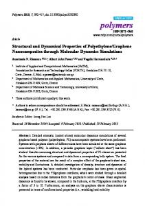
FIG. 1: The survival probability P (t) for the Bernoulli map at γ = γc = 0.2875 and for random and homogeneous absorbing states as a function of time t. Calculations were done for the threshold p = 10−10 (dashed line) and 10−16 (solid line). The upper straight dotted line have a slope which corresponds to the DP value δ = 0.1595 and for the lower line δ = 0.43.

the maximum simulation time. In such a way the spreading is never affected by finite size effects. Moreover, the data were averaged over 103 − 104 independent runs. Final results shown in Fig. 1 - Fig. 3 are obtained for γ = γc = 0.2875. Off-criticality the data deviate from the power law behaviour in a typical way. Estimating the asymptotic slope of our data we conclude that for the random synchronized state the exponents are in a good agreement with very accurately known DP values: δDP = 0.1595, ηDP = 0.3137, and z = 1.2652 [14]. However, in the case of homogeneous synchronized states, the exponents η and δ are clearly different and we estimate δ = 0.43(1) and η = 0.05(1). Let us notice that a very similar situation occurs in certain models with infinitely many absorbing states, where these critical exponents are also found to depend on the choice of an absorbing state [12]. Although the spreading exponents are nonuniversal in this class of models, they obey the following relation η + δ = ηDP + δDP .

(3)

It turns out that the estimated exponents for homogeneous synchronized states also obey this relation within an estimated error. From Eq. (3) and the hyperscaling relation [13] η+δ+Θ=

dz 2

(d = 1)

(4)

it follows that the exponent z must be constant and thus independent on the choice of the 5

0.6 0.4 0.2 log10[w(t)]

random 0 -0.2 -0.4

homogeneous

-0.6 -0.8 -1 0

FIG. 2:

0.5

1

1.5

2 log10(t)

2.5

3

3.5

4

The averaged difference w(t) as a function of time t for the Bernoulli map at γ = γc =

0.2875 and for random and homogeneous absorbing states. Calculations were done for the threshold p = 10−10 (dashed line) and 10−16 (solid line). The upper straight dotted line have a slope which corresponds to the DP value η = 0.3134 and for the lower straight line η = 0.05.

absorbing state. Indeed, in Fig. 3 one can see that both for the random and homogeneous absorbing states the asymptotic increase of R2 (t) is described by the same exponent. The main conclusion which follows from the above calculations is that synchronization should be considered as a transition in a model with multiple absorbing states rather than a single one. Except for non-DP values of η and δ it has essentially no other consequences in the one-dimensional case. For example all steady-state exponents keep the DP values. However, the situation might be different in higher-dimensional models with infinitely many absorbing states. In particular, there are some analytical and numerical indications that in such a case a non-DP criticality might appear [15].

B.

Symmetric Tent map

The second map examined by AP is the symmetric tent map defined as f (u) = 1 − 2|u − 1/2|,

(0 ≤ u ≤ 1). In this case they found that the synchronization transition belongs to

the BKPZ universality class and occurs at γ = γc = 0.17614(1). A qualitative difference between the critical behaviour in the case of Bernoulli and tent maps is attributed to the strong nonlinearity (i.e., discontinuity) of the first map. Another interesting feature reported by AP is a different behaviour of the transverse Lyapunov exponent λ⊥ . For the tent map 6

5 4.5 4 log10[R2(t)]

3.5 3 2.5 2 1.5 1 0.5 1

FIG. 3:

1.5

2

2.5 log10(t)

3

3.5

4

The average spread square R2 (t) as a function of time t for the Bernoulli map at

γ = γc = 0.2875 with random (solid line) and homogeneous (dashed line) absorbing states. The straight dotted line have a slope which corresponds to the DP value z = 1.2652.

λ⊥ vanishes exactly at γc , while for the Bernoulli map it vanishes inside a chaotic phase. For the tent map we also performed the spreading-dynamics calculations but only for random synchronized states. Our results for the time dependence of w(t) are shown in Fig. 4. The asymptotic decay of w(t) is described by the exponent η = −0.53(5) (note a minus sign). As for the estimation of δ our results strongly suggest that in this case δ = 0. Indeed, in the examined range of the threshold p we observed that all runs survived until the maximum measured time tm = 104 . From the behaviour of R2 (t) (Fig. 5) we estimate z = 1.30(5), which is in a good agreement with the expected KPZ value z =

4 3

[7, 16].

The hyperscaling relation provides a constraint on the exponents η, δ, Θ, and z. Since for the BKPZ universality class z is a simple number (4/3), it is tempting to assume that other exponents are also simple numbers. Thus we might speculate that in this model the exact value of η is -0.5. Then, from the hyperscaling relation (4) together with δ = 0 and z = we obtain Θ =

7 6

4 3

= 1.166 . . .. Such a value might be compared with numerical estimations

of this exponent which range from 1.1(1) [7, 16] to 1.26(3) [9].

7

-0.6 -0.8

log10[w(t)]

-1 -1.2 -1.4 -1.6 -1.8 -2 -2.2 0

FIG. 4:

0.5

1

1.5

2 2.5 log10(t)

3

3.5

4

4.5

The averaged difference w(t) as a function of time t for the symmetric tent map at

γ = γc = 0.17614 and for random absorbing states. Calculations were done for the threshold 10−10 . The least-square fit to the last decade date give η = −0.53(5). The dotted straight line has a slope which corresponds to η = −0.5. 4 3.5

log10[R2(t)]

3 2.5 2 1.5 1 1

1.5

2

2.5

3

3.5

log10(t)

FIG. 5:

The average spread square R2 (t) as a function of time t for the symmetric tent map

at γ = γc = 0.17614 and random absorbing states. The straight dotted line have a slope which corresponds to the KPZ value z = 1.3333. C.

Asymmetric Tent map

In this subsection we examine the asymmetric tent map defined as   au for 0 ≤ u < 1/a f (u) =  a(1 − u)/(a − 1) for 1/a ≤ u ≤ 1,

(5)

and 1 < a ≤ 2. For a = 2 this is the symmetric tent map. Let us notice that in the limit a → 1, the slope of the second part of this map diverges. Below we present the results of 8

0.05

L=104 L=103

0.04

w

0.03

0.02

0.01

0 0.18

0.19

0.2

0.21

0.22

0.23

γ

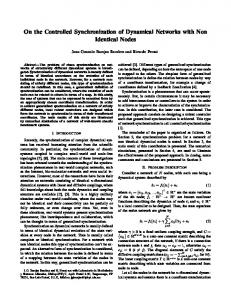
FIG. 6: The steady-state synchronization error w as a function of γ for the asymmetric tent map (a = 1.1). The measurement was made during t = 105 steps after 5 · 104 steps of relaxation. In the range (0.22 ≤ γ ≤ γc = 0.2288) w is well fitted with a power-law function a(γc − γ)β , where β = 1.5.

our calculations for a = 1.1, 1.02 and 1.01.

1.

a=1.1

When a is not too close to 1, model (1) remains in the BKPZ universality class. In particular, for a = 1.1 the estimated exponents β = 1.5(1) (Fig. 6) and Θ = 1.16(10) (Fig. 7) are in good agreement with other estimations for this universality class.

2.

a=1.02

However, for a close to 1 the nature of the transition changes. From the measurements of w (Fig. 8) and its time dependence w(t) (Fig. 9) we estimate that in this case γc = 0.17095 and Θ = 0.25(5). Using the spreading dynamics calculations for the random synchronized states at the critical point we estimate (Fig. 10 - Fig. 12): η = 0.15(3), δ = 0.27(2), and z = 1.32(3). All of the exponents, except z are far from the BKPZ values.

9

-2.5 -3

log10[w(t)]

-3.5 -4 -4.5 -5 -5.5 -6 2

2.5

3

3.5

4

4.5

log10(t)

FIG. 7: The time dependence of w for the asymmetric tent map (a = 1.1) and γ equal to (from top) 0.228, 0.2285, 0.2288 (critical), and 0.229. Calculations were done for L = 3 · 105 . The dotted straight line has a slope corresponding to Θ = 1.16. 0.0035 L=104 0.003

L=105

0.0025

w

0.002 0.0015 0.001 0.0005 0 0.166

0.168

0.17

0.172

γ

FIG. 8: The steady-state synchronization error w as a function of γ for the asymmetric tent map (a = 1.02). The measurement was made during t = 105 steps after 5 · 104 steps of relaxation. 3.

a=1.01

From the measurements of w (Fig. 13) and its time dependence w(t) (Fig. 14) we estimate that in this case γc = 0.13695 and Θ = 0.15(2). Similarly to the a = 1.02 our results for w close to the critical point are not sufficiently accurate to determine β. Using the spreading dynamics calculations for the random synchronized states at the critical point we estimate (Fig. 10-Fig. 12): η = 0.22(2), δ = 0.21(2), and z = 1.25(5). Again, the exponents, except z are far from the BKPZ values. However, Θ and z are consistent with the DP value. Moreover, the sum η + δ = 0.43 that is also quite close to the DP value (0.4732). Thus, it is 10

-3 -3.2

log10[w(t)]

-3.4 -3.6 -3.8 -4 -4.2 -4.4 2

2.5

3

3.5 log10(t)

4

4.5

5

FIG. 9: The time dependence of w for the asymmetric tent map (a = 1.02) and γ equal to (from top) 0.1707, 0.1709, 0.17095, 0.1710, and 0.1712. Calculations were done for L = 5 · 104 . We identify the central curve as critical. -0.5 -1 a=1.02 log10[w(t)]

-1.5 a=1.01 -2 -2.5 -3 -3.5 2

2.5

3

3.5

4

4.5

log10(t)

FIG. 10:

The averaged difference w(t) as a function of time t for the asymmetric tent map and

for random absorbing states. Calculations were done for a = 1.02 with γ = γc = 0.17095 and for a = 1.01 with γ = γc = 0.13695. The dotted straight lines have a slope which corresponds to η = 0.15 (upper) and η = 0.22 (lower).

in our opinion likely that in this case the model belongs to the DP universality class but the random synchronized states are not ”natural” absorbing states [12] and that is why η and δ separately do not take their DP values. Let us notice that for the Bernoulli map, examined in section III-A, the random synchronized states are probably a good approximation of the ”natural” absorbing states, since the obtained spreading exponents coincide the DP values. Our numerical results are summarized in Table I.

11

0 -0.2 a=1.02

log10[P(t)]

-0.4 -0.6 -0.8

a=1.01

-1 -1.2 2

2.5

3

3.5

4

4.5

log10(t)

FIG. 11: The survival probability P (t) for the asymmetric tent map with random absorbing states. Calculations were done for a = 1.02 with γ = γc = 0.17095 and for a = 1.01 with γ = γc = 0.13695. The dotted straight lines have a slope which corresponds to Θ = 0.27 (upper) and Θ = 0.21 (lower). 6 5.5 5

log10[R2(t)]

4.5

DP KPZ

4 3.5 3 2.5 2 1.5 1 0.5 1

1.5

2

2.5 3 log10(t)

3.5

4

4.5

FIG. 12: The average spread square R2 (t) as a function of time t for the asymmetric tent map and random absorbing states. Calculations were done for a = 1.02, γ = γc = 0.17095 (solid line) and a = 1.01, γ = γc = 0.13695 (dashed line). The straight dotted lines have slopes that correspond to DP and KPZ value of z. IV.

DISCUSSION

In this paper we studied the dynamical properties of CML models undergoing a synchronization transition. Our main results show that:(i) the synchronized state is not unique and (ii) non-BKPZ critical behaviour might appear for continuous maps. One of the open questions that we leave for the future is why for sufficiently asymmetric but continuous maps the linear analysis, that leads to the relation with BKPZ model, breaks down. For 12

0.004

L=104 L=105

0.0035 0.003

w

0.0025 0.002 0.0015 0.001 0.0005 0 0.133

0.134

0.135

0.136

0.137

0.138

γ

FIG. 13: The steady-state synchronization error w as a function of γ for the asymmetric tent map (a = 1.01). The measurement was made during t = 105 steps after 5 · 104 steps of relaxation. -3 -3.1

log10[w(t)]

-3.2 -3.3 -3.4 -3.5 -3.6 -3.7 2.5

3

3.5

4

4.5

5

log10(t)

FIG. 14:

The time dependence of w(t) for the asymmetric tent map (a = 1.01) and γ equal to

(from top) 0.1368, 0.13685, 0.1369, 0.13695, and 0.137. Calculations were done for L = 5 · 104 .

TABLE I: Critical parameters for the symmetric and asymmetric tent map. The last column shows how much the critcal exponents deviate from critical hyperscaling relation (4). z 2

a

γc

Θ

η

δ

β

z

η+δ

2

0.17614

1.26(3)

-0.53(5)

0.0(1)

1.50(5)

1.30(5)

–

0.07 (0.11)

1.1

0.2288

1.16(10)

–

–

1.5(1)

1.30(5)

–

–

1.02

0.17095

0.25(5)

0.15(3)

0.27(2)

?

1.32(3)

0.42

0.01 (0.11)

1.01

0.13695

0.15(2)

0.22(2)

0.21(2)

?

1.25(5)

0.43

0.04 (0.08)

DP

–

0.1595

0.3137

0.1595

0.2765

1.2652

0.4732

0

13

−Θ−η−δ

strongly asymmetric maps the (deterministic) noise is very large and this seems to be the only factor that might change the universality class. It is known that depending on how the noise scales with the order parameter, Langevin-type models, that presumably describe our model at criticality and at a coarsed-grained level might exhibit either DP or BKPZ critical behaviour [17]. In particular when the amplitude of noise scales linearly with the order parameter the model exhibits the BKPZ critical behaviour while the DP one for the square root scaling. Thus, the problem is to explain how a qualitatively different scaling of the noise in the Langevin-type model could emerge due to a more quantitative changes (in asymmetricity) in a coupled CML system. It is also tempting to expect that BKPZ and DP critical behaviours meet for a certain asymmetricity value ac (1.1 < ac < 1.01) at a new multi-critical point. Our estimation of Θ for a = 1.02 significantly deviates both from DP and BKPZ values which might be an indication of such a new critical point.

Acknowledgments

This work was partially supported by the Swiss National Science Foundation and the project OFES 00-0578 ”COSYC OF SENS”.

[1] H. Fujisaka and T. Yamada, Progr. Theor. Phys. 69, 32 (1983). A. S. Pikovsky, Z. Phys. B 55, 149 (1984). S. Boccaletti, J. Kurths, G. Osipov, D.l. Vallades and C.S. Zhou, Phys. Rep. 366 1-101 (2002). [2] R. Roy and K. S. Thornburg, Phys. Rev. Lett. 72, 2009 (1994). H. G. Schuster et al., Phys. Rev. A 33, 3547 (1984). W. Wang et al., Chaos 10, 248 (2000). [3] J. F. Heagy, T. L. Carroll, and L. M. Pecora, Phys. Rev. E 52, R1253 (1996). A. Amengual et al., Phys. Rev. Lett. 78, 4379 (1997). S. Boccaletti et al., Phys. Rev. Lett. 83, 536 (1999). [4] P. Grassberger, Phys. Rev. E 59, R2520 (1999). [5] Theory and Applications of Coupled Map Lattices, edited by K. Kaneko (John Wiley & Sons, Chichester, 1993) [6] A. S. Pikovsky and J. Kurths, Phys. Rev. E 49, 898 (1994). [7] Y .Tu, G. Grinstein, and M. A. Mu˜ noz, Phys. Rev. Lett. 78, 274 (1997).

14

[8] L. Baroni, R. Livi and A. Torcini, Phys. Rev. E 63, 036226 (2001). [9] V. Ahlers and A. S. Pikovsky, Phys. Rev. Lett. 88, 254101 (2002). [10] P. Grassberger, Z. Phys. B 47, 365 (1982). H. K. Janssen, ibid. 42, 151 (1981). [11] P. Grassberger and A. de la Torre, Ann. Phys. (N. Y.) 122, 373 (1979) [12] J. F. F. Mendes, R. Dickman, M. Henkel, and M. C. Marques, J. Phys. A 27, 3019 (1994). [13] For a general introduction into models with absorbing states see e.g., H. Hinrichsen, Adv. Phys. 49, 815 (2000). [14] I. Jensen, J. Phys. A 32, 5233 (1999). [15] F. van Wijland, e-print: cond-mat/0209202 (Phys. Rev. Lett. in press). [16] M. A. Mu˜ noz and T. Hwa, Europhys. Lett. 41, 147 (1998). [17] M. A. Mu˜ noz, Phys. Rev. E 57, 1377 (1998).

15