simulated in recent years using dynamic adaptive refinement (DARe). ... To sketch out the formalism, we consider the d-dimensional Burgers equation for ...
Dynamically adaptive computation of multiscale coherent-structure interactions using GASpAR Aim´e FOURNIER, Duane ROSENBERG, Annick POUQUET NCAR Institute for Mathematics Applied to Geosciences, USA We present the Geophysical/Astrophysical Spectral-element Adaptive Refinement (GASpAR) code [8] and use it to simulate vortices in decaying 2D turbulence. The adaption criteria suggest techniques for vortex and coherent-structure identification. We will explore how the multiresolution hierarchical structure of spectral elements also suggests a way to quantify interactions among different vortices and the incoherent background flow. Coherent-structure dynamics involves a large range of strongly interacting scales in space and time. Fronts, plumes and other structures in geophysical flows have been successfully simulated in recent years using dynamic adaptive refinement (DARe). There are a growing number of DARe codes and applications. All of these involve partitioning the SKsomehow ¯ ¯ computational spatial domain D into disjoint elements D = k=1 Ek . Almost all current DARe codes are based on finite-difference, finite-element or finite-volume spatial discretiza¯ k. tions; i.e., a small number of values is used to represent the problem solution in each E Thus almost all current DARe simulations are intrinsically locally low-order w.r.t. the size hk of each Ek . In contrast, there are a few DARe codes being developed that are locally high-order w.r.t. a parameter p~k in each Ek . These spectral-element methods (SEMs) have a relatively long history in engineering but have only recently been applied to astro/geophysics, particularly as relates to detailed studies of small scales. SEMs use degree-pαk polynomial expansions, defined by pαk +1 quadrature nodes along coordinate xα in Ek . For example, Fig. 1 shows one of the 36 Gauss interpolating basis functions φ˜~,k (~x) for D = E1 and p11 = p21 = 5. There are several properties of SEMs that make them very appropriate for complicated flow simulations. Perhaps most significant is the fact that unlike low-order methods, SEMs are inherently minimally diffusive and dispersive. This property is clearly important when trying to model flows at high Reynolds number Re (low viscosity) that characterize turbulent behavior. Also SEMs can be used in high-resolution studies of turbulence in domains with complicated boundaries. SEMs also are naturally parallelizable [e.g., 5], which is important for modeling high-Re flow with many degrees of freedom (d.o.f.) involving multiple spatial and temporal scales.
Figure 1: φ˜(3,3),1 .
SEMs are spectrally convergent w.r.t. pk when the solution is smooth in Ek , but are also effective when the solution is not smooth elsewhere. In most flows of interest, it is scale interaction that determines not only the structures that form but also their statistics and evolution. This suggests that reasonably high-pk approximations are required in each
element. Thus flows of interest mainly call for a nonconforming h-refinement strategy only, making use of relatively high, fixed degree. We note that globally continuous pk -refinement is possible using the so-called “mortar element method”, but this has been cited as causing instabilities in flow calculations [7]. To sketch out the formalism, we consider the d-dimensional Burgers equation for velocity ~u(t, ~x): ~ u = Re−1 ∇2~u ∂t~u + (~u · ∇)~ (1) We discretize by integrating (1) against a test function and then approximating by GaussLobatto quadrature, to arrive at a system of ODEs in time: M
duα + N(~ u)uα = Re−1 L uα , dt
α ∈ {1, . . . d},
(2)
where M is the mass matrix, uα is a column vector of collocated values on quadrature nodes, N(~ u) is the nonlinear-advection matrix, and L is the Laplacian. Continuity for ~u is imposed by reconciling element-boundary data among neighbor Ek s. Time discretization of (2) begins by standard semi-implicit split-multistep methods, but includes preconditioning issues beyond the present scope. SEM-DARe is enhanced w.r.t. low-order DARe in regard to adaptivity criterion. Since Qd α every Ek contains α=1 (pk + 1) local d.o.f., that information provides a local accuracy estimate. Possibilities that have been tested include estimating local Legendre-spectrum decay, or comparing relative contributions to the ~u-norm in L2 (Ek ) from Ek vs from its 2d children Ek0 by d-way bisection. The latter possibility is enabled by the multiresolution hierarchy intrinsic to SEM-DARe, i.e., (2(`+1)d −1)/(2d −1)−1 k
span φ~,k =: P ( ~
[ S2d (k+1)
k0 =2d k+1
P Ek0 =Ek
k0
⇒
[
Pk =: V` ( V`+1 ,
(3)
k=(2`d −1)/(2d −1)
as introduced in detail by Fournier [3]. The projection operator projV` \V`−1 on fine scales is the continuous spectral-element analog to the discontinuous spectral-element projection used by Fournier et al. [4], but is not orthonormal; nevertheless, it allows exact energy decomposition. These projections are rigorous analogs for spectral elements, of ideal Fourier spectral wavenumber bandpass filtering on uniform grids. Figure 2 shows snapshots at 4 times of the vorticity field ζ(t, ~x) for a 2D incompressible Navier-Stokes test case [6, 9] computed by GASpAR on a static uniform K = 32×32, pαk = 16 mesh. Based on (3), each of the 4 times (columns) in Fig. 2 can be analyzed a posteriori into the sum of the rows of Fig. 3. The field shown on each row interpolates to zero at any node of the elements in the preceding, higher row; this property takes the place of orthonormality. Note that initially ζ contains only large scales, but as the filaments are generated over time, smaller scales emerge. The next steps will be to utilize this multiresolution information for adaptivity, vortex extraction [1] and triadic interactions [2].
Figure 2: Vorticity ζ(t, ~x) field at t = 0, 8.5, 17, 25.5, from − π2 (blue) to 0 (white) to π (red).
References [1] M. Farge, K. Schneider and N.K.-R. Kevlahan 1999. Non-Gaussianity and coherent vortex simulation for two-dimensional turbulence using an adaptive orthogonal wavelet basis, Phys. Fluids 11, 2187–2201. [2] A. Fournier 2002. Atmospheric energetics in the wavelet domain I: Governing equations and interpretation for idealized flows, J. Atmos. Sci. 59, 1182-1197. [3] A. Fournier 2005. Adaptive multiresolution analysis on continuous spectral elements, in preparation. [4] A. Fournier, G. Beylkin and V. Cheruvu, 2005. Multiresolution adaptive space refinement in geophysical fluid dynamics simulation, Lecture Notes Comp. Sci. Eng. 41, 161–170. [5] A. Fournier, M.A. Taylor and J.J. Tribbia 2004. The spectral element atmosphere model (SEAM): High-resolution parallel computation and localized resolution of regional dynamics, Mon. Wea. Rev. 132, 726–748. [6] N.K.-R. Kevlahan and M. Farge 1997. Vorticity filaments in two-dimensional turbulence: Creation, stability and effect, J. Fluid Mech. 346, 49–76. [7] E.M. Rønquist 1996. Convection Treatment Using Spectral Elements of Different Order, Int. J. Num. Meth. Fluids 22, 241–264. [8] D. Rosenberg, A. Fournier, P. Fischer and A. Pouquet 2005. Geophysicalastrophysical spectral-element adaptive refinement (GASpAR): Object-oriented hadaptive code for geophysical fluid dynamics simulation, J. Comp. Phys. submitted, arxiv:math.NA/0507402. [9] K. Schneider, N.K.-R. Kevlahan and M. Farge 1997. Comparison of an adaptive wavelet method and nonlinearly filtered pseudo-spectral methods for two-dimensional turbulence, Theoret. Comput. Fluid Dynamics 9, 191–206.
Figure 3: Multiresolution analysis of Fig. 2. Row 1 shows projV0 ζ on the coarsest scale (1×1 element) and row ` + 1 > 1 shows projV` \V`−1 ζ on finer scales (2` × 2` elements).