Modular Model Checking of Dynamically Adaptive

Modular Model Checking of Dynamically Adaptive Programs∗ (Technical Report) Ji Zhang and Betty H.C. Cheng Software Engineering and Network Systems Laboratory Department of Computer Science and Engineering Michigan State University East Lansing, Michigan 48824 {zhangji9,chengb}@cse.msu.edu Abstract Increasingly, software must dynamically adapt its behavior in response to changes in its runtime environment and user requirements in order to upgrade services, to harden security, or to improve performance. In order for adaptive software to be used in safety critical systems, they must be trusted. In this paper, we introduce a sound approach for modularly verifying whether an adaptive program satisfies its requirements specified in temporal logics (LTL and A-LTL). Compared to existing model checking approaches for adaptive programs, our approach reduces the time/space complexity of verifying an adaptive program by a factor of n, where n is the number of steady-state programs encompassed by the adaptive program. Our approach is orthogonal to many other modular model checking approaches in that it can work in conjunction with other approaches to reduce the overall model checking cost of adaptive programs. We illustrate our technique on the specification and verification of an adaptive mobile computing application.

1 Introduction Increasingly, software must dynamically adapt its behavior in response to changes in its runtime environment and user requirements in order to upgrade services, to harden security, or to improve performance. In order for adaptive software to be used in safety critical systems, they must be trusted. In this paper, we introduce a sound approach for modularly verifying whether an adaptive program satisfies its requirements specified in temporal logics. Compared to existing adaptive program model checking approaches [1, 2], our approach has the following advantages: (1) It reduces the verification cost of adaptive programs by a factor of n, where n is the number of steady-state programs [1, 3] encompassed by the adaptive program. (2) Our verification technique can be applied incrementally to verify an adaptive system, leveraging previously verified results. Model checking has been previously used to verify properties of adaptive software [1, 2, 3]. A steady-state program is a state machine that we assume to be itself nonadaptive. An n-plex adaptive program M comprises n steady-state programs P 1 , P2 , · · · Pn , only one of which is running at a time. During execution, it is possible for M to adapt from running in one steady-state program to another. Critical properties of an adaptive program need to be verified including properties local to each steady-state program (local properties), properties that apply during adaptation from one steady-state program to another (transitional properties), and invariant properties that should be held by the adaptive program throughout its execution (global invariants). Since the number of steady-state programs in an adaptive program may be large, existing model checking approaches may be too complex (in terms of time and space complexity) to be applied to verify large scale adaptive programs. In addition, an adaptive program may be developed in a stepwise fashion as in extreme programming [4], where an (n + 1)th steady-state program may be incrementally developed after an n-plex adaptive program has been developed and verified; the model checking approach should be able to verify the adaptive program incrementally without repeating the model checking for the entire adaptive program. This paper proposes a modular model checking approach to address the above problems. We avoid directly model checking a large adaptive program by decomposing the task into smaller verification modules. First, we verify a set of base conditions ∗ This work has been supported in part by NSF grants EIA-0000433, EIA-0130724, ITR-0313142, CCR-9901017, CCF-0541131, and CNS-0551622, and the Department of the Navy, Office of Naval Research under Grant No. N00014-01-1-0744, and a Michigan State University Quality Fund Concept Grant.

1

using a traditional model checking approach [5, 6, 7, 8]. Second, for each steady-state program Pi , we calculate the guarantees, the necessary conditions for each steady-state program to satisfy its base conditions. Third, for each steady-state program P j , we calculate the assumptions, the sufficient conditions that each state of Pj must satisfy in order for Pj to satisfy transitional properties and/or global invariants. Then we prove that all the assumptions and guarantees can be directly or indirectly inferred from the set of base conditions, thus completing the overall verification process. Compared to existing approaches, our approach reduces the complexity of verifying an adaptive program by a factor of n, where n is the number of steady-state programs in the adaptive program. Moreover, when one steady-state program P i is modified or a new steady-state program Pn+1 becomes available after the remainder of the adaptive program has been verified using our approach, the model checking that needs to be repeated is limited to only Pi (and/or related adaptations). In this paper, we assume the steady-state programs are given as FSMs (Finite State Machines), specifically, Kripke structures [9]. Existing tools [10], including Bandera [11] and FLAVERS [12], process programs in high-level programming languages and generate state machines similar to what we need for our approach. We have proved (see appendix) the correctness of the proposed approach and implemented the algorithms in a prototype model checker AMO EBA (Adaptive program MOdular Analyzer) in C++. We have successfully applied AMO EBA to verify a number of adaptive programs developed for the RAPIDware project [14], including an adaptive TCP routing protocol [15] and an adaptive Java pipeline example [16]. The remainder of this paper is organized as follows. In Section 2, we introduce the verification problems using a simplified adaptive TCP routing protocol to illustrate the key verification challenges. Section 3 uses the example to illustrate the basic idea of our approach. We discuss optimizations, complexity, and limitations of our approach in Section 4. Section 5 describes an empirical study, and related work is overviewed in Section 6. Section 7 concludes this paper and briefly discusses our future directions.

2 Specifying Adaptive Systems In this section, we introduce a simplified version of an adaptive TCP routing protocol [15] developed for RAPIDware [14], an Office of Naval Research project that provides a concrete application for adaptive program verification challenges and is also used to illustrate our proposed solution.

2.1

Adaptive TCP Routing

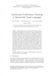
The adaptive TCP routing protocol is a network protocol involving adaptive middleware in which a node balances the network traffic by dynamically choosing the next hop for delivering packets. We assume two types of next hop nodes: trusted and untrusted. The protocol works in two different modes: safe and normal. In “safe” mode, only trusted nodes are selected for packet delivery, and in “normal” mode, both types are used in order to maximize throughput. Any packet must be encrypted before being transferred to an untrusted node. We consider the program running in the safe and normal modes to be two steady-state programs P 1 and P2 , respectively. Figure 1 shows the FSM for the adaptive protocol. For convenience, we assign a unique state name to each state. The upper rectangle in Figure 1 illustrates P1 . Initially, P1 is in the ready1 state, in which, P1 may receive a packet and move to state received1. At this point, P1 searches for a trusted next hop and moves to state routed1. Then P1 sends the packet to the next hop and goes to state sent1, and returns to the ready1 state. The lower rectangle in Figure 1 illustrates P 2 . The ready2, received2, and sent2 states are similar to those in P1 . In state received2, searching for the next hop may return a trusted or untrusted node, and thus P2 moves to the safe2 and unsafe2 states, respectively. From state unsafe2, P 2 tests whether the input packet has been encrypted. If the packet has been encrypted, then P2 goes to state encrypted2, otherwise, it goes to state unencrypted2. Then P 2 encrypts the packet and goes to the encrypted2 state. Four adaptive transitions are defined between P 1 and P2 : a1, a2, a3, and a4. We annotate (in italics) each state with the conditions that are true for the state (only the relevant conditions are shown). Critical properties of the adaptive program are specified in linear temporal logic (LTL) [17]. Global invariants are the properties that must be satisfied by an adaptive program regardless of adaptations. For the adaptive routing protocol, we require the program not to drop any packet throughout its execution, i.e., after it receives a packet, it should not receive the next packet before it sends the current packet. Formally in LTL: inv = 2(received ⇒ (¬ready U sent)). In addition to global invariants, each steady-state program has its local properties that may or may not be shared by other steadystate programs. In this example, we require P1 to never use an unsafe next hop. Formally in LTL, we write LP1 = 2(¬unsafe). For P2 , we require the system to encrypt a packet before sending the packet if the next hop is unsafe. Formally in LTL, we write LP2 = 2(¬safe ⇒ (¬sent U encrypted)).

2

Figure 1. Case study: adaptive routing protocol For an execution of an adaptive program, if it adapts (i.e., the control changes) among the steady-state programs of the adaptive program, then the execution must satisfy the corresponding local properties of the steady-state programs sequentially in the same order. Previously, we introduced the A-LTL (Adapt-operator extended LTL) [18] to specify the adaptation from satisfying one Ω LTL specification to satisfying another. For example, we write φ*ψ, where φ, ψ, and Ω are three LTL formulae, to mean that an execution initially satisfies φ; in a certain state A, it stops being constrained by φ, and in the next state B, it starts to satisfy ψ, and the two-state sequence (A, B) satisfies Ω.1 We can use Ω = InP1 to specify that the adaptation transition must emit from a Ω state within the program P1 . For simplicity, in this paper we assume Ω ≡ true and write φ*ψ instead of φ*ψ. However, our approach also applies to cases where Ω can be an arbitrary LTL formula (see appendix). In general, in an adaptive program with n steady-state programs P1 , P2 , ...Pn , any execution σj with a sequence of (k − 1) steps of adaptations, starting from Pj1 , going through Pj2 , · · · Pjk must satisfy LPj1 *LPj2 *LPj3 · · · *LPjk , where ji 6= ji+1 . We call this type of properties transitional properties. Note that each different adaptation sequence corresponds to a different transitional property. In practice, we have found A-LTL to be more convenient than LTL in specifying various adaptation semantics [18]. In theory, we can prove that while A-LTL and LTL have the same expressive power, A-LTL is at least exponentially more succinct than LTL in specifying transitional properties (even Ω ≡ true).2 Due to space constraints, we make its proof available in a technical report (see appendix). In the adaptive routing protocol, we express the transitional property that must be satisfied by executions adapting from P 1 to P2 with the A-LTL formula LP1 *LP2 , and the transitional property that must be satisfied by executions adapting from P1 to P2 and to P1 with the A-LTL formula LP1 *LP2 *LP1 , etc.

2.2

Verification Problems

Regarding an adaptive program, we must achieve two verification goals: (1) the global invariants hold for the adaptive program regardless of adaptations and (2) when the program adapts within its steady-state programs, the corresponding transitional properties are satisfied. Model checking techniques determine whether a program satisfies a given temporal logic formula by exploring the state space of the program. Numerous model checking techniques have been proposed to verify various properties of different types of programs. However, to the best of our knowledge, none of the existing verification approaches can be applied to verify adaptive programs efficiently (in terms of time and space complexity), which is discussed in the next section. 1 Note that the formal semantics of φ and Ω have been redefined to apply to state sequences with finite length; the theoretical discussion for this redefinition has been previously described [18] (also see appendix). 2 It is a common misunderstanding that the adapt operator in A-LTL can be simply replaced by the next or until operator in LTL. We have proved (see appendix) that it is not the case.

3

Global invariants. Allen et al [1] used model checking to verify that an adaptive program adapting between two steady-state programs satisfy certain global properties. While they do not explicitly address adaptations of n-plex adaptive programs (for n > 2), a straightforward extension could be to apply pairwise model checking between each pair of steady-state programs, separately. The first drawback of the pairwise extension is that it requires n2 iterations of model checking for a program with n steady-state programs. More importantly, this extension is theoretically unsound since it verifies executions with only one adaptation step, thus it does not guarantee the correctness of executions with more than one adaptation step. A sound solution proposed by Magee [19], called the monolithic approach [20], treats an adaptive program as a general program and directly verifies the adaptive program against its global invariants. The monolithic approach suffers from the state explosion problem: It is well known that the major limiting factor in model checking is the large amount of memory required by the computation [21]. However, most known efficient model checking algorithms have space complexity O(nlogn) [21], where n is the size (i.e., the number of states and transitions) of the program under verification. Although the example adaptive routing protocol has only two steady-state programs, the number can easily become very large in practice, and so can the required memory by the model checking computation. Furthermore, the monolithic approach is not suited for incremental adaptive software development. For example, after the adaptive routing protocol with two steady-state programs is verified, if a third steady-state program for a different condition becomes available by incremental development, then the monolithic approach cannot leverage the existing verification results. Instead, the entire verification must be repeated for the adaptive program with three steady-state programs. Transitional Properties. The transitional property verification is even more challenging. Since executions of an adaptive program may adapt within its set of steady-state programs in an infinite number of different sequences, the number of different transitional properties is also infinite. Therefore, it is impossible to verify each transitional property separately. To the best of our knowledge, no existing approaches address the transitional property verification problem defined in this paper. In order to address the above problems, we propose a sound modular model checking approach for adaptive programs against their global invariants and transitional properties that not only reduces verification complexity by a factor of n, where n is the number of steady-state programs, but also further reduces verification cost by supporting verification of incrementally developed adaptive software.

3 Modular Verification This section introduces a modular approach to the model checking of adaptive programs, where the verification result of an adaptive program can be derived from the model checking results of its individual steady-state programs. Our modular model checking uses the assume/guarantee reasoning [10, 20, 22, 23], where for a given program module (i.e., a steady-state program), the assumptions are the conditions of the running environment of the module that are assumed to be true, and guarantees are the assurances provided by the module under the assumptions. We first verify a set of base conditions in each steady-state program locally by using a traditional model checking approach [5, 6, 7, 8]. Second, for each steady-state program Pi we calculate the guarantees, the necessary conditions for each steady-state program to satisfy its base conditions locally. Third, for each steady-state program Pj , we calculate the assumptions, the sufficient conditions that each state of Pj must satisfy in order for Pj to satisfy transitional properties and/or global invariants. Fourth, we determine whether the guarantees logically imply the assumptions. If so, we conclude that all the assumptions and guarantees can be directly or indirectly inferred from the set of base conditions, thus completing the verification. Otherwise, a counterexample is generated.

3.1

Illustrating Our Approach

We illustrate our proposed approach using the adaptive routing protocol by applying it first to verify the global invariants and then to verify the transitional properties of the adaptive routing protocol. The detailed model checking algorithms and formal discussion (e.g., proofs of soundness) are included in the appendix. 3.1.1 Global Invariant Verification The global invariant verification proceeds as follows: 1. Verify base conditions: Verify each steady-state program against the global invariants individually. 2. Compute guarantees: Mark each state of the steady-state programs with conditions that are satisfied by those states when there is no adaptation. 3. Compute assumptions: Mark each state of the steady-state programs with conditions that must be satisfied by the state in order for the adaptive program to satisfy the global invariants. 4

4. Compare guarantees with assumptions: If the guarantees imply the assumptions, then the process returns success. Otherwise, it returns with a counterexample. (1) Verify base conditions. In this step, we verify each steady-state program against the global invariants individually. Since the global invariants are LTL formulae and we assume each steady-state program to be non-adaptive itself, we use an existing LTL model checking algorithm provided by Spin [24] to verify the base conditions. By model checking, we determine that both P 1 and P2 satisfy the invariant inv separately. (The detailed description of the process is included in the appendix.) (2) Compute guarantees. Next, we use a marking algorithm (see appendix for details) to mark each state of the steady-state programs with obligations, i.e., conditions satisfied by the state when there is no adaptation. The obligations are true in each state if the steady-state program comprising the state has passed the base condition verification in step (1). In the adaptive routing protocol, since P1 satisfies inv, we conclude that state ready1 satisfies inv, therefore, we mark ready1 with the obligation inv. Then we propagate this obligation to its successor state(s) received1 as follows: First, it satisfies inv. Second, since received is true in the state, it must also satisfy ¬ready U sent. Therefore, we mark received1 with obligations inv and ¬ready U sent. Similarly, the markings of states are repeatedly propagated to their successors. When a new obligation is propagated to an already marked state through a different execution path and the new obligation is not in the existing marking of the state, the state marking will be updated with the conjunction of the existing marking and the new obligation, otherwise the new obligation is ignored. This process will eventually converge (see appendix) and at that point (fixpoint), no state markings will be updated any further. Figure 2 shows P1 , the result of applying the marking algorithm, where the guarantee markings are prefixed with g.*. Similarly, we apply the marking algorithm to P2 ; results in bottom of Figure 2.

Figure 2. Markings for global invariant inv In our algorithm, the obligations are propagated in such a way that guarantees each state satisfies all the obligations in its markings when there is no adaptation. We call these markings guarantee markings. We can prove (see appendix for the proof) that at the fixpoint, the markings of a steady-state program Pi have the following property, which is a key insight of this paper: When a state machine Pj is connected to a state s in Pi with transitions from s to states in Pj , all the states of Pi still satisfy their guarantees if and only if s still satisfies its guarantee (3) Compute assumptions. Starting from the guarantee markings generated in step (2), for each state in each steady-state program Pi (the source) with outgoing adaptive transitions, we propagate the obligations along the adaptive transitions until reaching states of a target steady-state program Pj , then we mark the reached states in Pj with the propagated obligations, which we call the assumption markings. In the adaptive routing protocol, we propagate the markings of received1 to state received2 along the adaptive transition a1 and mark received2 with inv and ¬ready U sent. Our process ensures that the assumption marking includes exactly the set of conditions that received2 must satisfy in order for all executions starting from ready1, taking adaptive transition a1, and taking no more adaptations, to satisfy the global invariant inv. Similarly, we propagate the marking of routed1 to unsafe2, from received2 to received1, and from unsafe2 to routed1, respectively. The assumption markings are shown in Figure 2, prefixed with a.*.

5

P1: Safe Mode g.[] ! unsafe

g.[] ! unsafe

g.[] ! unsafe

g.[] ! unsafe

ready1

received1

routed1

sent1

a.(L P 2 L P 1 ) ∧(!s e n t U e n cr y p te d  L P 1 )

g.LP2/\ !sent U encrypted

P2: Normal Mode g.LP2

g.LP2

g.LP2/\ !sent U encrypted

ready2

received2

unsafe2

unencrypted2 g.LP2 encrypted2

g.LP2

g.LP2 sent2

safe2

Figure 3. Markings for transitional properties (4) Compare guarantees with assumptions. Next we compare the guarantees with the assumptions. For each state, if the conjunction of its guarantee marking logically implies all the conditions in its assumption marking (checked automatically), then the process returns success, otherwise, it returns with a counterexample. For example, the guarantee marking for received2 indeed implies the assumption marking for received2. This result implies that all executions starting from ready1, taking adaptive transition a1, with no adaptation afterwards, satisfy inv. We perform the comparison on every state of the steady-state programs with incoming adaptive transitions. Successful comparisons guarantee that any execution starting from ready1 or ready2, undergoing one step of adaptation, satisfies inv. We can inductively prove that inv is also satisfied by all executions with finite numbers of steps of adaptations (see appendix for the proof). If the guarantee of a state does not imply its assumption, then we generate a counterexample showing the path violating the global invariant. The counterexample feature is illustrated in the discussion for the transitional properties below. 3.1.2 Transitional Properties The steps for transitional properties verification are similar to those used for global invariants. The first two steps are the same as the first two steps used for global invariant verification except that the LTL formulae upon which we operate this time are the local properties LP1 and LP2 instead of inv. The last two steps will be described in detail below. (1’) Verify base conditions. This step is the same as step (1) for global invariants except that we model check the local properties instead. (2’) Compute guarantees. This step is the same as step (2) for global invariants except that we compute guarantees by starting with marking the initial states with local properties. The guarantee markings after applying steps (1’) and (2’) are shown in Figure 3, prefixed with g.*. (3’) Compute assumptions. In this step, we start from the guarantee markings generated in the previous step. For each state in a steady-state program Pi with outgoing adaptive transitions going towards program Pj , we generate an obligation φ*LPj from each condition φ in its guarantee marking, where LPj is the local property for Pj . Then we propagate the generated obligations to the states in Pj along the adaptive transitions to form their assumption markings. For example, the guarantee marking for unsafe2 is LP2 and (¬sent U encrypted). From this marking, we generate obligations LP2 *LP1 and (¬sent U encrypted)*LP1 respectively. These obligations are propagated to the state routed1, then we generate the assumption marking LP 2 *LP1 and (¬sent U encrypted)*LP1 for routed1. We repeat this process for all states in P1 and P2 with outgoing adaptive transitions, and the resulting assumption markings are shown in Figure 3, prefixed with a.*. (4’) Compare guarantees with assumptions. We compare the assumption markings with the guarantee markings of all states to see whether the assumptions are implied by the guarantees. If so, then the model checking returns success, otherwise, it returns a counterexample. We can prove (see appendix for the proof) that if the process returns success, then all adaptive executions with finite steps of adaptations satisfy their corresponding transitional properties. In the adaptive routing protocol, we find that the guarantee for state routed1 (LP1 ) does not imply the condition (¬sent U encrypted)*LP1 in its assumption. This assumption condition requires the obligation encrypted to be satisfied before the adaptation, while the guarantee does not ensure this obligation. Therefore, the model checking for the transitional property fails. As such, we generate a 6

counterexample showing a path that violates the transitional properties by using a backtracking method. In this example, we return the trace (ready2, received2, unsafe2, routed1). Clearly, the failure is caused by the adaptive transition a3 (from unsafe2 to routed1). We remove a3 from the adaptive program and re-perform steps (3’) and (4’). The algorithm returns success.

4 Discussion Next, we discuss performance issues including optimizations, scalability, and limitations.

4.1

Optimizations

The algorithm introduced in Section 3.1 stores in memory the guarantee and assumption markings of all the states in the adaptive program, which may occupy a large amount of memory. However, in later steps, only markings of a small portion of the states are used, i.e., the states with incoming and outgoing adaptive transitions. We call these states interface states, and the assumption/guarantee markings of these states assumption/guarantee interfaces, respectively. In the AMO EBA implementation, the required memory space is significantly reduced by storing the markings for only the interface states instead of for all the states during the marking computations (see appendix for details). Our approach can also be optimized to verify incrementally developed software by utilizing existing verification results. Assume that an n-plex adaptive program has been successfully verified with our approach. Consider the case when an (n + 1) th steady-state program Pn+1 is incrementally developed for the adaptive program. In order to verify the properties of the (n + 1)-plex adaptive program, we use our approach to only incrementally verify Pn+1 and the steady-state programs to which Pn+1 is connected with adaptive transitions/states.

4.2

Complexity and Scalability

Our proposed modular model checking approach increases scalability of model checking by reducing the time/space complexity of the model checking algorithms. We explain this point by comparing our approach to the alternative approaches that we described in Section 2, namely, the pairwise approach [1] and the monolithic approach [19, 20]. Assume an n-plex adaptive program M contains steady-state programs P1 , P2 , · · · , Pn . We denote the size of the steady-state program Pi as | Pi |, and we assume all steady-state programs are of similar size | P |: | P |≈| Pi |, for all i. We assume that the size of adaptive states and transitions are significantly smaller than the steady-state programs (which we consider a key characteristic of adaptive software). Then we have | M |≈ n ∗ | P |, where | M | is the size of M. The complexity of the global invariant model checking is the sum of the complexity of each step introduced in Section 3.1. The most time/space consuming step is computing the assumption and guarantee interfaces. We can prove that its time complexity is O(2|INV| | M |) and its space complexity is O(2|INV| | P |) (see appendix for details). The time and space complexities of the monolithic approach are both O(2|INV| | M |). That is, while the monolithic approach requires the same order of time, it requires n times more memory space than our approach. The time and space complexities of the pairwise approach are O(n(2 |INV| | M |)) and O(2|INV| | P |), respectively. That is, while it requires the same order of space, it requires n times more execution time than our approach. The time and space complexities of our transitional property model checking algorithm are O(2 |LP| | M |) and O(2|LP| | P |), respectively (see appendix for details). To the best of our knowledge, no alternative approach solves the same problem. The approach that handles the closest problem is the ITL model checking algorithm proposed by Thompson and Bowman [25], which can be applied to verify that executions of only a specific adaptation sequence satisfy their corresponding transitional property, instead of all possible adaptation sequences as with our approach. The memory consumption of their approach is linear to the size of the program automaton, which implies that our approach is at least n times more efficient in terms of space. In addition, their approach is non-elementary to the length of the equivalent A-LTL formulae, while our approach is exponential, which means that our approach is at least exponentially more efficient. Based on the above analysis, we conclude that our approach reduces the verification space/time complexity by a factor of n, and it is more scalable for verifying incremental changes to the adaptive program at development time.

4.3

Limitations

The following assumption must be considered when applying our approach: We regard the essential characteristic of an adaptive program to be that the n steady-state programs are loosely coupled, i.e., the size of adaptive states and transitions are significantly smaller than the size of the steady-state programs. This assumption is reasonable since it is generally desirable software engineering practice to minimize the coupling among program modules [26]. This condition ensures that both the number of markings that we need to store and the comparisons between interface markings that we need to perform are minimal. If the number of adaptive states and transitions is comparable to the size of the adaptive program, then our approach performs similarly to other (non-modular) model checking techniques. 7

5 Empirical Study In this section, we illustrate the performance improvement of our approach over existing approaches by applying it to a more complex case study: the adaptive Java pipeline program [16]. In some multi-threaded Java programs, such as proxy servers, data are processed and transmitted from one thread to another in a pipelined fashion. The Java pipeline is implemented using a pair of piped I/O classes, and the synchronization between the input and output classes is implemented using Java synchronized functions. Previously we have studied optimization techniques and proposed an asynchronous Java pipeline design to be run on a multi-processor machine. By eliminating synchronization overhead, the asynchronous version gains a speed up rate of 4.83 over the synchronized implementation when the CPU load is low. However, when the CPU load is high, the synchronized version performs better. Based on the above observations, we would like to build an adaptive version of the Java pipeline classes where the program can choose to use the optimal implementations at runtime based on the CPU workload. However, the complexity of designing a verifiably correct algorithm that switches between synchronization protocols prevented us from implementing the adaptive version of the program using traditional development techniques. With the approach introduced in the paper, we are able to not only build an adaptive program model, but also check critical properties, and therefore, gain confidence in the design of the adaptive program. Figure 4 shows the simplified adaptive Java pipeline state machine (with 2 data buffers). The label of each state is a pair: The first element (ranging from 0 to 2) represents the number of buffers already occupied by data (where 0 represents empty and 2 represents full); the second element is a status indicator including rlocked, wlocked, unlocked, reading, writing, where rlocked/wlocked means that the buffers are locked by a reader/writer thread, and reading/writing means that the pipeline is being read/written by a reader/writer thread. Transitions are labeled with wlock?, wlock!, rlock?, rlock!, w?, w!, r?, and r!, where rlock?/wlock? represents acquiring a read/write lock, and rlock!/wlock! represents releasing a read/write lock. r?/w? represents starting a read/write operation, and r!/w! represents completing a read/write operation.

P1

0,rlocked rlock?

1,reading

rlock!

1, rlocked

r?

r!

rlock?

0, unlocked

r! 2,reading

rlock!

Legend:

2, rlocked

r?

initial state

rlock? rlock!

1, unlocked

2, unlocked

wlock? wlock!

wlock? wlock!

state adaptive transition

wlock?

wlock!

0,wlocked

0,wrting w?

1,wrting

w?

w!

w!

1, wlocked

r? r!

2, wlocked

ȕ

Į

w? w!

P2

0, writing

1,idle

w!

w?

r?

0,idle

1, writing

w?

rlock?

w!

r?

2,idle r!

r! 1, reading

w?

1,

r! w!

r? 2, reading

wlock? rlock! wlock!

start reading end reading start writing end writing acquiring read lock acquiring write lock releasing read lock releasing write lock

Figure 4. Case study: Adaptive Java pipeline The upper rectangle in this figure illustrates P1 , the synchronized Java pipeline. In the initial state (0,unlocked), the buffer is empty and unlocked. The buffers can be locked by the reader/writer, and the program goes to (0,rlocked)/(0,wlocked). When the buffer is not empty/full, and a rlock/wlock is set, a read/write operation can be performed, and the operation must not interleave with any other operations until it completes. The lower rectangle in Figure 4 shows the asynchronous Java pipeline state machine. In this version, no lock is required, and the reader/writer can start reading/writing while the other is still in action. In the state (1, hwriting, readingi), both the write and read operations are active. We define two adaptive transitions: α and β connecting the two steady-state programs. Although more adaptive transitions are possible, for brevity, we only discuss this pair of adaptive transitions in the paper. Also for brevity, only global invariants are discussed in this paper as follows: • Buffer integrity: The program must not read (resp. write) while the buffer is empty (resp. full).

8

inv1

=

2(empty ⇒ ¬r?).

inv2

=

2(full ⇒ ¬w?).

• Lock integrity: After locking (rlock?/wlock?) the buffer, the reader/writer should eventually unlock (rlock!/wlock!) it before it can be locked by the other type of lock. inv3

=

2(rlock? ⇒ ¬wlock? U rlock!).

inv4

=

2(wlock? ⇒ ¬rlock? U wlock!).

• Read/write integrity: After the program starts reading/writing, it should complete reading/writing before the next reading/writing starts. inv5

=

2(r? ⇒ (¬r? U r!)).

inv6

=

2(w? ⇒ (¬w? U w!)).

We have successfully verified all of the above properties with the AMO EBA model checker. In order to study the scalability of our approach, we synthesized a series of n-plex adaptive programs by duplicating the above steady-state programs n/2 times (where n ranges from 2 to 200), and connecting these duplicates with adaptive transitions. We measured the execution time and memory consumption and compared the results to the monolithic and the pairwise implementations introduced in Section 2. The experimental results were evaluated on a dual processor 800MHZ Pentium III SMP with 32KB L1 and 256KB L2 caches, and 256MB main memory, running Redhat Linux 7.2. Figure 5(a) shows the experimental results of the average execution time of model checking for the above 6 global invariants, where the x-axis represents the number of steady-state programs in the adaptive programs and the y-axis represents the time elapsed during executions. From the results we noticed that the time consumed by our approach is linear to the number of steady-state programs. It is about n times faster than the pairwise approach, and slightly slower than the monolithic approach. Figure 5(b) shows the memory usage where the x-axis represents the number of steady-state programs in the adaptive programs and the y-axis represents the memory occupied by the program in the numbers of states stored by the algorithms during model checking. From these results, we can see that our approach uses almost constant amount of memory, which is approximately only 1/n of the amount of memory required by the monolithic approach and 1/2 of the memory required by the pairwise approach. The above results conform to the theoretical complexity analysis discussed in Section 4.2.

execution time in seconds

(a) Execution time changes with number of steady-state programs 50

AMOebA monolithic pairwise

40 30 20 10 0 2

40

80

120

160

200

number of steady-state programs

memory usage in number of state

(b) Memory usage changes with number of steady-state programs 600

AMOebA monolithic pairwise

400 200 0 2

40

80

120

160

200

number of steady-state programs

Figure 5. Empirical study: performance comparison between our approach and the monolithic and the pairwise approaches

6 Related Work This section compares our approach with existing modular verification techniques of non-adaptive programs and non-modular verifications of adaptive programs. 9

6.1

Modular Model Checking

Our work has been significantly influenced by several existing modular model checking approaches for non-adaptive programs. In this section, we focus on the analysis of the differences and relationships between our approach and other modular verification approaches. Krishnamurthi, et al [10] introduced a modular verification technique for aspect-oriented programs. They model a program as a finite state machine (FSM), where an aspect is a mechanism used to change the structure of the program FSM. An aspect includes a point-cut designator, which defines a set of states in the program, an advice, which is an FSM itself, and an advice type, which determines how the program FSM and the advice FSM should be composed. By model-checking the program and the aspect individually, they verify Computation-Tree Logic (CTL) properties of the composition of the program and the aspect. In their other work [27, 28] they introduced modular model checking techniques for cross-cutting features. Similar to our approach, their approach deals with the verification of behavior changes; however, their focus is on verifying design time changes, i.e., the composition of the program and the features occurs before run time. Once the program starts, the program executes either with or without the feature. They do not handle run-time adaptations from programs with (resp. without) a feature to those without (resp. with) the feature. Another difference between their approach and ours is that they check CTL properties instead of LTL/A-LTL properties; these are complementary logics (branching time v.s. linear time). We consider our approach to be complementary to theirs in the sense that, for example, if we want to verify an adaptation from program P “without” an aspect (or feature) A to “with” A, then we can first verify the local properties before and after composing A with P using their approach. Then we can verify the transitional properties and global invariants using our approach. Henzinger et al [4] proposed using the Berkeley Lazy Abstraction Software verification Tool (BLAST) to support extreme verification (XV). XV is modeled to be a sequence of program and specifications (Pi , Φi ), where Φi is the specification for the ith version of the program Pi , and Φi are non-decreasing, i.e., Φi ⊆ Φi+1 . In order to reduce the cost of each incremental verification when verifying the ith program, they generate an abstract reachability tree Ti . When model-checking Pi+1 , they compare Pi+1 to Ti to determine the part of Pi+1 , if any, should be re-verified. Our approach differs in that they verify propositional, instead of temporal logic properties. Also, their approach is for general programs, while our incremental verification is optimized specifically for adaptive programs. Again, we consider their approach and ours to be complementary because, in practice, each steady-state program is developed incrementally from some common base program. Their approach can verify the local properties and global invariants of each steady-state program locally for the base condition verification. Alur et al [29] introduced an approach to model-checking a hierarchical state machine, where higher-level state machines contain lower-level state machines. As the same state machine may occur at different locations in the hierarchy, its model checking may be repeated if we flatten the hierarchical state machine before applying traditional model checking. Their objective is to reduce the verification redundancy when a lower-level state machine is shared by a number of higher level state machines. Their approach can be applied to optimize our solution in that the steady-state programs may share parts of their behavior (sub-state machines). We can use their approach to reduce the redundancy when verifying the shared behavior. Many others, including Kupferman and Vardi [30], Flanagan and Qadeer [31], have also proposed modular model checking approaches for different program models. They focus on verifying concurrent programs, where modules are defined to be concurrent threads (processes). Their approaches essentially address a different perspective of model checking problems (e.g., data sharing among threads), and we consider their approaches to be orthogonal and complementary to our approach.

6.2

Correctness in Adaptive Programs

Model checking has been applied to verify adaptive behavior by several researchers. Kramer and Magee [2] used Darwin to describe architectural views and used FSP to model the behavioral views of an adaptive program. They used property automata to specify the properties for the adaptive program and used LTSA to verify these properties. Allen et al. [1] integrated the specifications for both the architectural and the behavioral aspects of dynamic programs using the Wright ADL. They use two separate component specifications to describe the behavior of a component before and after adaptation and encapsulate the dynamic changes in the “glue” specification of a connector, thus achieving separation of concerns. The Wright specifications are converted into the process algebraic language, CSP [32], which then are statically verified. In our previous work [3], we introduced a model-based adaptive software development process that uses Petri nets to model the behavior of each steady-state program and adaptive states and transitions separately, and then uses existing model checking tools to verify these models against interesting properties. None of the above approaches address the verification problem modularly. Compared to these approaches, the modular model checking approach proposed in this paper is less complex, more scalable, and supports not only LTL, but also A-LTL. Many others have also worked on providing assurance to adaptive systems. Kramer and Magee [33] introduced the notion of quiescent state, i.e., the state in which connections to a component can be changed safely. They described an algorithm to ensure that the system is in a quiescent state when a component is removed. Chen et al [34] proposed a graceful adaptation protocol that 10

allows adaptations to be coordinated across hosts transparently to the application. Appavoo et al [35] proposed a hot-swapping technique, i.e., run-time object replacement. Previously, we [36] also introduced a centralized algorithm to ensure safeness in adaptive software while minimizing cost associated with adaptation. These approaches provide safe adaptation protocols based on runtime dependency analysis, instead of model checking approaches as proposed in this paper. Theorem-proving techniques have also been explored by researchers to verify adaptive programs. Kulkarni et al [37] introduced an approach using proof-lattice to verify that all possible adaptation paths do not violate global propositional constraints. Their approach differs from ours in that first, they use theorem-proving, and second, they check propositional properties instead of temporal properties.

7 Conclusions and Future Work In this paper, we introduced a sound modular approach to model-checking adaptive programs against their global invariants and transitional properties expressed in LTL/A-LTL. For an n-plex adaptive program, given that the size of the adaptive states and transitions is usually significantly smaller than the size of the overall adaptive program, our approach is at least n times more efficient than alternative approaches. Also, our approach is applicable to the transitional properties which, previously, had not been analyzable with other approaches. Our approach is highly scalable in that the time complexity is linear to the number of steady-state programs, and the space complexity is linear to the size of each steady-state program. More performance improvement can be achieved by using our approach to incrementally verify adaptive programs. For validation purposes, we have implemented our approach in a prototype model checker AMO EBA using C++, and used the tool to verify a number of adaptive programs. We note the potential for improving model checking performance by combining our approach with existing techniques [1, 2, 4, 10, 27, 28, 29, 30, 31, 32]. We are investigating strategies to combine our approach with others to further reduce the complexity of adaptive program model checking. Run-time verification of adaptive programs against their global invariants and transitional properties [38] is also part of our ongoing work.

References [1] R. Allen, R. Douence, and D. Garlan, “Specifying and analyzing dynamic software architectures,” in Proceedings of the 1998 Conference on Fundamental Approaches to Software Engineering (FASE’98), (Lisbon, Portugal), March 1998. [2] J. Kramer and J. Magee, “Analysing dynamic change in software architectures: a case study,” in Proc. of 4th IEEE International Conference on Configuratble Distributed Systems, (Annapolis), May 1998. [3] J. Zhang and B. H. C. Cheng, “Model-based development of dynamically adaptive software,” in Proceedings of International Conference on Software Engineering (ICSE’06), (Shanghai,China), May 2006. [4] T. A. Henzinger, R. Jhala, R. Majumdar, and M. A. Sanvido, “Extreme model checking,” Verification: Theory and Practice, Lecture Notes in Computer Science 2772, Springer-Verlag, pp. 332–358, 2004. [5] R. Gerth, D. Peled, M. Vardi, and P. Wolper, “Simple on-the-fly automatic verification of linear temporal logic,” in Proceedings of the Fifteenth IFIP WG6.1 International Symposium on Protocol Specification, Testing and Verification (PSTV95), (Warsaw, Poland), June 1995. [6] M.Y.Vardi and P. Wolper, “An automata-theoretic approach to automatic program verification,” in Proceedings of the 1st Symposium on Logic in Computer Science, (Cambridge, England), pp. 322–331, 1986. [7] P. Wolper, M. Vardi, and A. Sistla, “Reasoning about infinite computation paths,” in Proceedings of 24th Symposium on Foundations of Computer Science, pp. 185–194, IEEE Computer Society, Nov 1983. [8] M. Y. Vardi and P. Wolper, “Reasoning about infinite computations,” Inf. Comput., vol. 115, no. 1, pp. 1–37, 1994. [9] E. A. Emerson, “Temporal and modal logic,” Handbook of theoretical computer science (vol. B): formal models and semantics, pp. 995– 1072, 1990. [10] S. Krishnamurthi, K. Fisler, and M. Greenberg, “Verifying aspect advice modularly,” in SIGSOFT ’04/FSE-12: Proceedings of the 12th ACM SIGSOFT International Symposium on Foundations of Software Engineering, (New York, NY, USA), pp. 137–146, ACM Press, 2004. [11] J. C. Corbett, M. B. Dwyer, J. Hatcliff, S. Laubach, C. S. Pˇasˇareanu, Robby, and H. Zheng, “Bandera: extracting finite-state models from java source code,” in ICSE ’00: Proceedings of the 22nd International Conference on Software Engineering, (New York, NY, USA), pp. 439–448, ACM Press, 2000. [12] M. B. Dwyer and L. A. Clarke, “Flow analysis for verifying specifications of concurrent and distributed software,” Tech. Rep. Report UM-CS-1999-052, University of Massachusetts, Computer Science Department, August 1999. [13] J. Zhang and B. H. C. Cheng, “Modular model checking of dynamically adaptive programs,” Tech. Rep. MSU-CSE-06-18, Computer Science and Engineering, Michigan State University, East Lansing, Michigan, March 2006. http://www.cse.msu.edu/˜zhangji9/ Zhang06Modular.pdf.

11

[14] “RAPIDware.” http://www.cse.msu.edu/rapidware/. Software Engineering and Network Systems Laboratory, Department of Computer Science and Engineering, Michigan State University, East Lansing, Michigan. [15] C. Tang and P. K. McKinley, “Improving mutipath reliability in topology-aware overlay networks,” in Proceedings of the Fourth International Workshop on Assurance in Distributed Systems and Networks, (Columbus, Ohio), June 2005. [16] J. Zhang, J. Lee, and P. K. McKinley, “Optimizing the Java pipe I/O stream library for performance,” in Proceedings of the 15th International Workshop on Languages and Compilers for Parallel Computing (LCPC), Published as Lecture Notes in Computer Science (LNCS), Vol. 2481, Springer-Verlag, (College Park, Maryland, USA), July 2002. [17] A. Pnueli, “The temporal logic of programs,” in Proceedings of the 18th IEEE Symposium on Foundations of Computer Science, pp. 46–57, 1977. [18] J. Zhang and B. H. C. Cheng, “Using temporal logic to specify adaptive program semantics,” Journal of Systems and Software (JSS), Architecting Dependable Systems, vol. 79, no. 10, pp. 1361–1369, 2006. [19] J. Magee, “Behavioral analysis of software architectures using ltsa,” in Proceedings of the 21st International Conference on Software Engineering, pp. 634–637, IEEE Computer Society Press, 1999. [20] J. M. Cobleigh, G. S. Avrunin, and L. A. Clarke, “Breaking up is hard to do: an investigation of decomposition for assume-guarantee reasoning,” in ISSTA’06: Proceedings of the 2006 International Symposium on Software Testing and Analysis, (New York, NY, USA), pp. 97–108, ACM Press, 2006. [21] C. Courcoubetis, M. Vardi, P. Wolper, and M. Yannakakis, “Memory-efficient algorithms for the verification of temporal properties,” Formal Methods in System Design, vol. 1, no. 2-3, pp. 275–288, 1992. [22] C. B. Jones, “Tentative steps toward a development method for interfering programs,” ACM Transactions on Programming Languages and Systems (TOPLAS), vol. 5, no. 4, pp. 596–619, 1983. [23] B. Jonsson and Y.-K. Tsay, “Assumption/guarantee specifications in linear-time temporal logic,” Theoretical Computer Science, vol. 167, no. 1-2, pp. 47–72, 1996. [24] G. J. Holzmann, The SPIN Model Checker: Primer and Reference Manual. Addison-Wesley, 2003. [25] H. Bowman and S. J. Thompson, “A tableaux method for Interval Temporal Logic with projection,” in TABLEAUX’98, International Conference on Analytic Tableaux and Related Methods, no. 1397 in Lecture Notes in AI, pp. 108–123, Springer-Verlag, May 1998. [26] J. Offutt, M. J. Harrold, and P. Kolte, “A software metric system for module coupling,” The Journal of Systems and Software,Elsevier, vol. 20, pp. 295–308, March 1993. [27] K. Fisler and S. Krishnamurthi, “Modular verification of collaboration-based software designs,” in ESEC/FSE-9: Proceedings of the 8th European Software Engineering Conference held jointly with the 9th ACM SIGSOFT International Symposium on Foundations of Software Engineering, (New York, NY, USA), pp. 152–163, ACM Press, 2001. [28] H. Li, S. Krishnamurthi, and K. Fisler, “Verifying cross-cutting features as open systems,” ACM SIGSOFT Software Engineering Notes, vol. 27, no. 6, pp. 89–98, 2002. [29] R. Alur and M. Yannakakis, “Model checking of hierarchical state machines,” ACM Trans. Program. Lang. Syst., vol. 23, no. 3, pp. 273–303, 2001. [30] O. Kupferman and M. Y. Vardi, “Modular model checking,” in COMPOS’97: Revised Lectures from the International Symposium on Compositionality: The Significant Difference, (London, UK), pp. 381–401, Springer-Verlag, 1998. [31] C. Flanagan and S. Qadeer, “Thread-modular model checking,” in SPIN 03: SPIN Workshop, LNCS 2648, pp. 213–225, Springer-Verlag, 2003. [32] C. A. R. Hoare, Communicating sequential processes. Upper Saddle River, NJ, USA: Prentice-Hall, Inc., 1985. [33] J. Kramer and J. Magee, “The evolving philosophers problem: Dynamic change management,” IEEE Trans. Softw. Eng., vol. 16, no. 11, pp. 1293–1306, 1990. [34] W.-K. Chen, M. A. Hiltunen, and R. D. Schlichting, “Constructing adaptive software in distributed systems,” in Proc. of the 21st International Conference on Distributed Computing Systems, (Mesa, AZ), April 16 - 19 2001. [35] J. Appavoo, K. Hui, C. A. N. Soules, et al., “Enabling autonomic behavior in systems software with hot swapping,” IBM System Journal, vol. 42, no. 1, p. 60, 2003. [36] J. Zhang, B. H. C. Cheng, Z. Yang, and P. K. McKinley, “Enabling safe dynamic component-based software adaptation,” Architecting Dependable Systems, Lecture Notes in Computer Science, pp. 194–211, 2005. [37] S. Kulkarni and K. Biyani, “Correctness of component-based adaptation,” in Proceedings of International Symposium on Component-based Software Engineering, May 2004. [38] K. Havelund and G. Rosu, “Monitoring Java programs with Java PathExplorer,” in Proceedings of the 1st Workshop on Runtime Verification, (Paris, France), July 2001.

12

[39] J. Zhang and B. H. C. Cheng, “Specifying adaptation semantics,” in WADS ’05: Proceedings of the 2005 workshop on Architecting dependable systems, (St. Louis, Missouri), pp. 1–7, ACM Press, May 2005. [40] W. Thomas, “Automata on infinite objects,” Handbook of theoretical computer science (vol. B): formal models and semantics, pp. 133–191, 1990. [41] T. Wilke, “Classifying discrete temporal properties,” in STACS’99 (C. Meinel, ed.), vol. 1563 of Lecture Notes in Computer Science, (Trier, Germany), pp. 32–46, Springer, 1999. [42] R. Rosner and A. Pnueli, “A choppy logic,” in 1st IEEE Symposium on Logic in Computer Science, pp. 306–313, 1986. [43] D. Harel, D. Kozen, and R. Parikh, “Process logic: Expressiveness, decidability, completeness.,” Journal of Computer and System Sciences, vol. 25, no. 2, pp. 144–170, 1982. [44] O. Lichtenstein and A. Pnueli, “Checking that finite state concurrent programs satisfy their linear specification,” in Proceedings of the 12th ACM SIGACT-SIGPLAN symposium on Principles of programming languages, pp. 97–107, ACM Press, 1985. [45] P. K. McKinley, S. M. Sadjadi, E. P. Kasten, and B. H. C. Cheng, “Composing adaptive software,” IEEE Computer, vol. 37, no. 7, pp. 56–64, 2004. [46] J. Zhang, Z. Yang, B. H. C. Cheng, and P. K. McKinley, “Adding safeness to dynamic adaptation techniques,” in Proceedings of ICSE 2004 Workshop on Architecting Dependable Systems, (Edinburgh, Scotland, UK), May 2004.

13

A Appendix A.1

The Adapt-Operator Extended LTL

A.1.1 A-LTL Syntax To specify adaptation behavior, we have introduced A-LTL (Adaptive LTL) by extending LTL [17] with the adapt operator Ω (“*”) [39, 18]. The φ, ψ, and Ω are three temporal logic formulae named the source specification, the target specification and Ω the adaptation constraint of the formula, respectively. Informally, a program satisfying “φ *ψ” means that the program initially satisfies φ. In a certain state A, it stops being constrained by φ, and in the next state B, it starts to satisfy ψ, and the two-state Ω sequence (A, B) satisfies Ω. We used φ*ψ to specify the adaptation from a steady-state program that satisfies φ to another that satisfies ψ. More succinctly, we define A-LTL as follows: • If φ is an LTL formula, then φ is also an A-LTL formula. Ω

• If φ and ψ are both A-LTL formulae, and Ω is an LTL formula, then ξ = φ*ψ is an A-LTL formula. • If φ and ψ are both A-LTL formulae, then ¬φ, φ∧ψ, φ∨ψ, 2φ (always), ♦φ (finally), and φ U ψ (until) are all A-LTL formulae.

A.1.2 A-LTL Semantics A temporal logic may be interpreted over finite or an infinite state sequences. For example, LTL is interpreted over infinite sequences [17], while the choppy logic and ITL are interpreted over finite sequences [25]. We have defined A-LTL semantics over both finite state sequences (denoted by “|=fin ”) and infinite sequences (denoted by “|=inf ”). • Operators (→, ∧, ∨, 2, ♦, U , ¬, etc) are defined similarly as those in LTL. • If σ is an infinite state sequence and φ is an LTL formula, then σ satisfies φ in A-LTL if and only if σ satisfies φ in LTL. Formally, σ |=inf φ iff σ |= φ in LTL. • If σ is a finite state sequence and φ is an A-LTL formula, then σ |=fin φ iff σ 0 |=inf φ, where σ 0 is the infinite state sequence constructed by repeating the last state of σ. Ω

• σ |=inf φ*ψ iff there exists a finite state sequence σ 0 = (s0 , s1 , · · · sk ) and an infinite state sequence σ 00 = (sk+1 , sk+2 , · · ·), such that σ = σ 0 _ σ 00 , σ 0 |=fin φ, σ 00 |=inf ψ, and (sk , sk+1 ) |=fin Ω, where φ, ψ, and Ω are A-LTL formulae, and the _ is the sequence concatenation operator. Ω

Informally, a sequence satisfying φ*ψ can be considered the concatenation of two subsequences, where the first subsequence satisfies φ, the second subsequence satisfies ψ, and the two states connecting (“_”) the two subsequences satisfy Ω. For convenience, we define empty to be the formula that is true on only single state sequences, i.e., deadlock states: empty ≡ ¬ true [25]. A.1.3 A-LTL and LTL are equivalent in expressive power An ω-automaton is a finite state automaton that accepts ω-words [40]. Two most popular forms of ω-automata are B¨uchi automata and Muller automata [40]. It has been shown that B¨uchi automata and Muller automata are equivalent [40]. An ω-automaton is counter-free if it does not contain counters [41]. Wilke had shown that LTL is equivalent to counter-free ω-automata and introduced an algorithm to convert a counter-free automaton to an LTL formula [41]. In this paper, we establish the equivalence between LTL and A-LTL by showing that A-LTL is also equivalent to counter-free automaton. The above statements also apply to finite words [41]. 14

Theorem 1 A-LTL is equivalent to counter-free automata Proof 1 We need to prove (1) any A-LTL can be accepted by a counter-free B¨uchi automaton and (2) any counter-free B¨uchi automaton can be expressed by an A-LTL formula. (1) We prove by induction on the number of nested adapt “*” operators in a formula. Initial condition: Any A-LTL formula with 0 adapt operator is also an LTL formula, which can be accepted by a counter-free ω-automaton in ω-word domain, and can be accepted by a counter-free FSA in finite word domain. Assumption: Any A-LTL formula with no more than k nested adapt operators can be accepted by a counter-free (ω) automaton. Ω For an A-LTL formula with k + 1 nested adapt operator, it can be decomposed into φ *ψ, where φ and ψ have no more than k nested adapt operator. Based on the assumption, we can build an FSA A for φ in finite words domain and a counter-free ωautomata B for ψ in ω-word domain. Then we connect the accepting states of A to the initial states of B and make all states in A true non-accepting to form an ω-automaton C. Clearly C accepts the set of executions that satisfy φ *ψ. By selectively connecting the accepting states of A and the initial state of B, we can make sure all the state pairs satisfy Ω. The resulting ω-automaton accepts Ω exactly the set of sequences satisfying φ*ψ. The same process applies to A-LTL in finite words domain. Now we show C is also counter-free. Since A and B are counter free, if there is a counter in C, the counter must include states both in A and in B. Since there is no transition from B to A, such counter cannot exist. Therefor, C is counter-free. Therefore, any A-LTL formula with no more than k + 1 nested adapt operators can be accepted by a counter-free (ω) automaton. (2) Any counter-free automaton can be expressed in LTL, and any LTL formula is also an A-LTL formula in ω-words domain. Therefore, any counter-free automaton can be expressed in A-LTL We say a logic L1 is more expressive than another logic L2 , denoted L1 ≥ L2 , if and only if for any formula φ2 in L2 , there exists a formula φ1 in L1 such that φ1 accepts exactly the same set of models that φ2 accepts. We say a logic L1 is strictly more expressive than another logic L2 , denoted L1 > L2 , if and only if L1 ≥ L2 , but L2 6≥ L1 . We say L1 and L2 are equivalent in expressive power, denoted L1 ≡ L2 , if and only if L1 ≥ L2 and L2 ≥ L1 . The expressiveness of TA-LTL is defined in terms of the set of timed state sequences that satisfy each TA-LTL formula. Theorem 2 A-LTL is equivalent to LTL in expressive power: A-LTL ≡ LTL Proof 2 We prove that A-LTL is more expressive than LTL and vice-versa. (1) A-LTL is more expressive than LTL: TA-LTL ≥ A-LTL. The proof of this statement is straightforward. Since A-LTL is a super set of LTL, for any formula φ of LTL, there is also a formula φ0 of exactly the same form in A-LTL, and φ0 = φ. Therefore, we have A-LTL ≥ LTL (1) LTL is more expressive than A-LTL: LTL ≥ A-LTL. For any formula φ in A-LTL, we can build a counter-free automaton that accepts exactly the set of words S that satisfy φ (Theorem 1). And thus, there exists an LTL formula φ0 that accepts S. Then we have LTL ≥ A-LTL  A.1.4 A-LTL is at least exponentially more succinct than LTL While A-LTL and LTL are equivalent in expressive power, we have found A-LTL to be convenient compare to express various adaptation semantics [18]. We also found in many cases, the A-LTL formulae are is much more intuitive than the corresponding LTL formula. For example, if we want to express adapting from a program satisfying 2(A→♦B) to a program satisfying 2(C→♦D), in A-LTL we write 2(A→♦B)*2(C→♦D), which directly captures the intent. The equivalent LTL formula is

15

(A→♦(B∧♦2(C→♦D))) U (2(C→♦D) which is much more confusing. As a matter of fact, we can prove that A-LTL formulae are at least exponentially more succinct than LTL formulae. Ω The adapt operator * in A-LTL is closely related to the chop operator ; in the choppy logic [42, 43], and ITL [25]. The chop operator is defined as follows: • σ |=c φ;ψ if and only if exists finite sequence σ1 and infinite sequence σ2 , such that σ1 |=c φ, σ2 |=c ψ, and σ = σ1 ◦ σ2 , where ◦ is a fusion operator [42]. Any choppy logic formula can be expressed in A-LTL in at mostVdouble exponential length. Any choppy logic formula ψ with k nested chop operators can be decomposed into a normal form (pi ∧ qi ) in which pi are propositions and qi are choppy logic formulae with no more than k nested chop operators. For a choppy logic formula with k + 1 nested chop operator φ;ψ, we V V ( decompose ψ into (pi ∧ qi ), then we convert φ;ψ into (φ*pi )qi ). This process may continue until all chop operators are converted into adapt operators. In each conversion, the number of conjuncts is bounded by 2H , where H is the number of atomic propositions. Therefore the length of the generated A-LTL formula is bounded by 2HL , where L is the number of nested chop operators. Theorem 3 A-LTL is at least exponentially more succinct than LTL, i.e., the length of an LTL formula equivalent to an A-LTL formula may be exponentially longer than the A-LTL formula. Proof 3 It as been shown that the most efficient algorithm for temporal logics with chop operator known so far has non-elementary complexity, i.e., the exponential height equals to the depths of nested chop operators [42, 25]. However, the most efficient LTL model checking algorithm is exponential to the length of the formulae. Assume there is a conversion function that converts any A-LTL φ formula to LTL formula of length less or equal to O(2 |φ| ), |φ| whose model checking complexity is O(22 ). For an arbitrary choppy logic formula ψ, let the equivalent A-LTL formula be φ, 2HL

and we have the length of φ is | φ |= O(2HL ). Therefore the corresponding LTL formula will be of length O(22 ), which conflicts with the best known model checking complexity for the choppy logic. Therefore, there is no such a conversion from A-LTL to LTL of length no more than exponential, i.e., A-LTL is more than exponentially succinct than LTL. 

B Adaptive Program Models and Verification In this section, we introduce a formal model for adaptive programs, and formally state the verification problem. In model checking, a program is usually modeled as a finite-state machine (or a Kripke structure) [9, 44]. We also use finite-state machines as the formal models for adaptive programs in that an adaptive program is essentially a program, where we would like to reuse existing techniques and theories developed for finite-state machines. However, adaptive programs are a special type of programs, i.e., they change their behavior in response to environment and requirements changes [45]. We explore their regularities by analyzing the behavior of each steady-state program individually, and infer properties of the adaptive program behavior. We define the formal models for adaptive programs in the next section.

B.1

The Formal Models

Given a set of atomic propositions AP, a finite-state machine (FSM) is a triple M = (S, S 0 , T, L), where S is a set of states, transitions T : S × S is a set of state pairs, where (s, t) ∈ T represents that there is an arc from s (the predecessor) to t (the successor). The initial state set S0 ⊆ S is a subset of the states. The function L : S → 2AP labels each state s with a set of atomic propositions that are evaluated true in s. We represent the states, the transitions, the labels, and the initial states of a given labeled transition system M with S(M), T(M), L(M), and S0 (M), respectively. The states in M that do not have a successor state are deadlock states, denoted D(M). We can remove the deadlock states in an FSM by introducing a self-loop to each deadlock state. An FSM is an extended FSM (EFSM) if it does not contain a deadlock state. 16

We formally model an n-plex adaptive program as an EFSM that contains n steady-state programs P 1 , P2 , · · · , Pn , each of which is an EFSM, and there exist adaptations among the Pi s. Each steady-state program represents a different program behavior for a runtime execution domain. We require that these steady-state programs be state disjunct, i.e., no two steady-state programs may share any state. This can be achieved by simply introducing an atomic proposition to identify each steady-state program. The adaptation from Pi (the source program) to Pj (the target program) is modeled by an adaptation set Ai,j . An adaptation set contains the intermediate states and transitions connecting one steady-state program to another, representing a collaborative adaptation procedure, such as the insertion and removal of filters [36, 46]. An adaptation set is formally defined as an FSM with the following features: • All initial states are states in the source program: S0 (Ai,j ) ⊆ S(Pi ). • All deadlock states are states in the target program: D(Ai,j ) ⊆ S(Pj ). • No transition should return from the adaptation set to the source program: ∀ s, t : S(Ai,j ), (s, t) ∈ T(Ai,j ) ⇒ t 6∈ S(Pi ). • No transition should return from the target program to the adaptation set: ∀ s, t : S(Ai,j ), (s, t) ∈ T(Ai,j ) ⇒ s 6∈ S(Pj ). • There should be no cycles in the adaptation set. This condition ensures the adaptation integrity constraint [3]. That is, the adaptation should finally reach a state of the target program. • No two adaptation sets may share the same states other than those in the target and source programs. We define the composition of two programs comp(Pi , Pj ) to be a program with all the states and transitions in Pi and Pj , and with initial states coming from only Pi : comp(P , P ) = (S, S , T, L), where i

j

0

S

=

S(Pi ) ∪ S(Pj ), T = T(Pi ) ∪ T(Pj ),

L

=

L(Pi ) ∪ L(Pj ), and S0 = S0 (Pi ).

The comp operation can be recursively extended to accept a list of programs:

comp(Pi1 , Pi2 , · · · Pin ) = comp(comp(Pi1 , Pi2 ), Pi3 , · · · , Pin ). (1) Similarly, we define the union of two programs union(Pi , Pj ) to be a program with all the states, transitions, and initial states from Pi and Pj . union(P , P ) = (S, S , T, L), where i

j

0

S

=

S(Pi ) ∪ S(Pj ), T = T(Pi ) ∪ T(Pj ),

L

=

L(Pi ) ∪ L(Pj ), S0 = S0 (Pi ) ∪ S0 (Pj )

The union operation can be extended to accept a list of programs:

union(Pi1 , Pi2 , · · · Pin ) = union(union(Pi1 , Pi2 ), Pi3 , · · · , Pin ). (2) A simple adaptive program SAi,j from program Pi to Pj includes the source program Pi , the target program Pj , and the adaptation set Ai,j that comprises the intermediate states and transitions connecting Pi to Pj . Formally, we define the simple adaptive program from program Pi to Pj to be the composition SAi,j = comp(Pi , Ai,j , Pj ). (3) An n-plex adaptive program M contains the union of all the states, transitions, and initials states of n steady-state programs and the corresponding adaptation sets. Formally: M = comp(union(P1 , · · · pn ), union(A1,2 , A1,3 , · · · An,n−1 )). (4) An execution of an n-plex adaptive program M is an infinite state sequence s0 , s1 , s2 · · · such that si ∈ S(M), (si , si+1 ) ∈ T(M), and s0 ∈ S0 (M) (for all i ≥ 0). A non-adaptive execution is an execution s0 , s1 , s2 · · ·, such that all its states are within one program si ∈ Pj , for all si and some Pj . An adaptive execution is any execution that is not non-adaptive. An adaptive execution goes through one or more adaptation transitions, and two or more steady-state programs. For an A-LTL/LTL formula φ, an execution sequence σ of an adaptive program satisfies φ if and only if σ |= φ. Conventionally, we say a state s of an adaptive program satisfies a formula φ (i.e., s |= φ) if and only if all execution paths initiated from s satisfy φ. And an adaptive program M satisfies φ (i.e., M |= φ), if and only if all its initial states satisfy φ. In addition, for convenience, we define a formula mapping function Ψ : S0 → A-LTL/LTL that assigns each initial state a formula. We say M satisfies Ψ (i.e., M |= Ψ), q if for any initial state s0 ∈ S0 (M), we have s0 |= Ψ(s0 ) . 17

B.2

Verification Problem Statement

Assume that we are given an n-plex adaptive program M with steady-state programs P1 , P2 , · · · , Pn , and adaptation sets Ai,j , for some i, j (i 6= j). Also assume that we are given a local property φi for each steady-state program, and global invariant properties INV for the n-plex adaptive program M, all written in LTL. We want to verify the following properties by model checking: • For an arbitrary execution σi initiated from program Pi1 , with k − 1 (k ≥ 2) times of adaptation through Pi2 , Pi3 , · · · Pik where ij 6= ij+1 satisfies φi1 *φi2 · · · *φik , that is sequentially satisfying φi1 · · · φik . • Any execution of M with k (k ≥ 0) times of adaptation satisfies INV.

B.3

Algorithms and Data Structure

This section introduces preliminary notations, algorithms, and a basic data structure that are required by our model checking algorithm. We define an obligation of a program state s of a program P to be a necessary condition that the state must satisfy in order for the program to satisfy a given temporal logic formula ρ. In this section, we introduce an algorithm that marks each state of a program with a set of obligations. Intuitively, the algorithm first marks the initial states of P with obligation ρ, then the obligations of each state are propagated to its successor states in a way that preserves the necessary conditions along the propagation paths. If a state is reachable from the initial states from more than one path, then the obligations of the state is the conjunction of the necessary conditions propagated to the state along all these paths. B.3.1 Partitioned Normal Form The logic closest to A-LTL is the ITL studied by Bowman and Thompson [25]. They have introduced using the Partitioned Normal Form (PNF) [25] to support model checking ITL properties. In our work, we also use the Partitioned Normal Form (PNF) [25] to handle obligation propagation. We rewrite each A-LTL/LTL formula into its PNF as follows: _ (pe∧empty)∨ (pi ∧ qi ), (5) i The (pe∧empty) part of the PNF form depicts the condition when Wa sequence is empty, where empty ≡ ¬ true [25], and pe is a proposition that must be true when the state is the last state. In the i (pi ∧ qi ) part of the formula, the propositions pi partitions true, and qi is the corresponding condition that must hold when pi holds in the current state. Formally, pe, pi and qi satisfy the following constraints:

• pe and pi are all propositional formulae W • pi partitions true, i.e., i pi ≡ true and pi ∧pj ≡ false for all i 6= j. All A-LTL/LTL formulae can be rewritten in PNF by applying PNF-preserving rewrite-rules [25]. The negation rule: ¬φ

= (¬pφe ∧empty)∨

_

(pφi ∧ ¬qφi )

(6)

The conjunction rule: φ∧ψ

= (empty∧(pφe ∧pψ e ))∨

__ i

φ ψ (pφi ∧pψ j )∧ (qi ∧qj )

(7)

φ ψ ((pφi ∧pψ j )∧ (qi ∨qj ))

(8)

j

The disjunction rule: φ∨ψ

= (empty∧(pφe ∨pψ e ))∨

__ i

The next rule: 18

j

φ

= (empty∧false)∨(true∧ φ)

(9)

The global rule: 2φ

= (empty∧pe )∨

_

(pi ∧ (qi ∧2φ))

(10)

♦φ

= (empty∧pe )∨

_

(pi ∧ (qi ∨♦φ))

(11)

The eventuality rule:

The until rule: φU ψ

= (empty∧pψ e )∨

__ i

The adapt rule:

Ω

φ*ψ

=

φ ψ φ (pψ i ∧pj ∧ (qi ∨qi ∧φ U ψ))

(12)

j

(empty∧false)∨ __ φ Ω φ (pi ∧pj ∧peφ ∧ ((qΩ j ∧ψ)∨(qi *ψ)))∨ i

_

j

(pφi ∧¬peφ ∧ (qφi *ψ)),

i

where φ and ψ are A-LTL formulae, and we use superscripts on pi , qi and pe to represent the formula from which they are constructed. Since pe and pi are all propositions, their truth values can be directly evaluated over the label of each single state. Therefore, the obligations of a given state can be expressed solely by a next state formula: the q i part of a disjunct when the state has successor states, and/or empty in case the state is a deadlock state. B.3.2 Property Automaton Bowman and Thompson’s [25] tableau construction algorithm first creates a property automaton based on an initial formula φ, and then constructs the product automaton of the property automaton and the program. Their approach is suited for verifying that all initial states satisfy the same initial formula. However, our model checking algorithm requires us to mark program states with necessary/sufficient conditions for different initial states to satisfy different initial formulae in the assumption computation step. We could create a different property automaton for each formula, but it would have duplicated states. Instead, we extend their property automaton construction algorithm to support multiple initial formulae for our purpose as follows. The property automaton construction algorithm: A property automaton is a tuple (S, S 0 , T, P, N), where S is a set of states. S0 is a set of initial states where S0 ⊆ S. T : S → 2S maps each state to a set of next states. P : S → proposition represents the propositional conditions that must be satisfied by each state. N : S → formula represents the conditions that must be satisfied by all the next states of a given state. Given a set of A-LTL/LTL formula Φ, we generate a property automaton PROP(Φ) with the following features: • For each member φ ∈ Φ, create an initial state s ∈ S0 such that P(s) = true, N(s) = φ. • For each state W s ∈ S, let the PNF of N(s) be (pe∧empty)∨ i (pi ∧ qi), then it has a successor s0i ∈ S for each pi field with P(s0i ) = pi and N(s0i ) = qi . A path of a property automaton is an infinite sequence of states s0 , s1 , · · · such that s0 ∈ S0 , sn ∈ S, and si , si+1 ∈ T, for all i (0 ≤ i < n). We say a path of a property automaton s0 , s1 , · · ·, simulates an execution path of a program s01 , s02 , · · ·, if P(si ) agrees with s0i for all i (0 < i). We say a property automaton accepts an execution path from initial state s ∈ S 0 , if there is a path in the property automaton starting from s that simulates the execution path. It can be proved [13] that the property automaton constructed above, from initial state s ∈ S0 , accepts exactly the set of executions that satisfy N(s).3 3 We

ignore the eventuality constraint [6] (a.k.a self-fulfillment [44]) at this point. However, later steps will ensure eventuality to hold in our approach.

19

B.3.3 Product Automaton Construction and Marking Our algorithm handles the case when each initial state of a program P is required to satisfy a different A-LTL/LTL formula. Given a program P = (SP , SP0 , T P , LP ) and a formula mapping function Ψ : SP0 → A-LTL/LTL, we use the following algorithm to mark the states of P with sufficient/necessary conditions in order for P to satisfy Ψ. We can prove that the algorithm works for calculating both assumptions and guarantees. A product automaton is defined to be a tuple: Q = (SQ , SQ0 , T Q ), where SQ is a set of states with two fields: (pstate, nextform). The pstate field represents one state of program P. The nextform field contains an A-LTL/LTL formula declaring what should be true in the next state. S Q0 is a set of initial states, SQ0 ⊆ SQ . T Q is a set of transitions, T Q : SQ × SQ . Given a program automaton P, and a mapping function Ψ from its initial states to a set of A-LTL/LTL formulae, we generate a product automaton PROD(P, Ψ) as follows: 1. Calculate the relational image of the initial states of P under the mapping function Ψ. Φ = {φ | ∃ s ∈ S0 , φ = Ψ(s)}. 2. Construct a property automaton PROP(Φ) with the set of initial formulae Φ using the property automaton construction algorithm introduced in Section B.3.2. 3. For each initial state of the program si ∈ SP0 , add a pseudo program state psi (a program state that was not originally in the state space SP ) and a transition (psi , si ) to P, and label psi with LP (psi ) = true. 4. For each pseudo program state psi , create an initial product state sQ0 , where sQ0 ∈ SQ0 and sQ0 = (psi , φ). 5. Create the cross product of P and PROP(Φ) from the above initial states [6, 25]. Marking states: Given a program P and an initial formula mapping function Ψ, we first construct the product automaton PROD(P, Ψ), then we construct the marking of each program state MARK(s) to be the set of nextform fields of states in PROD(P, Ψ) that correspond to s. Our marking algorithm generates the function MARK over selected states. We also applied optimizations to the algorithm so that we do not need to store the entire product automaton. Theorem 4 The marking algorithm will terminate. Proof 4 The markings of each state is a subset of formulae in the property automaton, i.e., the number of formulae in each marking is finite. Also the number of states in the property automaton is also finite. We repeatedly check all nodes to see whether there will be update to the node. For each iteration, we have two possible outcomes: 1. No change to the markings: The process terminates. 2. At least one for formula is added to the marking of a state: We will repeat the process. Since the number of nodes is finite and the number of markings is finite and the total number of formulae in all the states markings strictly increases by 1 at each iteration, the process will have only finite number of iterations until it eventually terminate. The markings generated by the marking algorithm contribute to the assumptions and guarantees in our model checking approach. We can prove that the marking of a state contains the necessary conditions that the state must satisfy in order for the program to satisfy Ψ [13]. Theorem 5 For a program P with initial states S0 and an initial formula mapping function Ψ, let MARK be the marking for the V states generated using the marking algorithm above, and let θ be the conjunction of the marking of a state s, θ = MARK(s), then P satisfies Ψ implies that s satisfies θ. That is V (P |= Ψ) ⇒ (s |= MARK(s)) Lemma 1 A path π of a property automaton A simulates an execution σ, then σ |= N(π 0 ) iff σ 1 |= N(π1 ). Proof 5 this is a direct result of building theWproperty automaton according to the PNF for a formula. π simulates σ, we have π 1 agrees with σ0 . Let N(π0 ) be (pe∧empty)∨ i (pi ∧ qi ), without losing generality, we assume P(π1 ) = p1 , and N(π1 ) = q1 . We have σ |= N(π0 ) ⇔ σ |= q1 . Therefore, σ |= N(π0 ) iff σ 1 |= N(π1 ) 20

Lemma 2 A path π of a property automaton A simulates an execution σ, then σ |= N(π 0 ) iff σ i |= N(πi ). Proof 6 This is an inductive result of Lemma 1. Proof 7 Now we prove Theorem 5. Prove by Contradiction: V Assume that s does not satisfy θ, then there exists a path σ from s such that σ 6|= θ. θ = M(s), then there exists formula φ ∈ M(s), σ 6|= φ. φ ∈ M(s) implies that (s, φ) is reachable by a path π in the product automaton starting from some s 0 ∈ S0 and Ψ(s0 ). Let σ 0 be the finite execution corresponding to π, from Lemma 2, we have σ 0 _ σ |= Ψ(s0 ) ⇔ σ |= φ. Given that the program satisfies Ψ, we have σ |= φ: a contradiction. In fact, we can also prove that for a state s, if s satisfies all the formulae in the marking of s, then all paths starting from s i ∈ S0 going through s satisfy Ψ(si ) [13]. Theorem 6 For a program P with initial states S0 and an initial formula mapping V function Ψ, using the marking procedure above, for any state s of P, let θ be the conjunctions of all the marking of s: θ = MARK(s), then s satisfies θ implies all paths of P starting from si ∈ S0 , going through s satisfy Ψ(si ). Proof 8 Prove by contradiction. Assume s |= θ and exists a path of P σ starting from si ∈ S0 , going through s and σ 6|= Ψ(si ). Let s be the jt h state in σ and Let π be the path in the product automaton corresponding to σ. From Lemma 2 We have σ |= N(π0 ) ⇔ σ j |= N(πj ). N(πj ) must be a conjunct in θ, therefore, we have s |= N(πj ), and thus σ j |= N(πj ). Then we have σ |= N(π0 ), which implies σ |= Ψ(si ), a contradiction. Now, we prove the key insight of this paper. This insight allows us to connect two steady-state programs without repeat the entire verification. Theorem 7 For a program Pi with initial states S0 and an initial formula mapping function Ψ, using the marking procedure V above,for any state s of P, let θ be the conjunctions of all the marking of s: θ = MARK(s). Let Pj be a state machine. Let P be the state machine including Pi , Pj and transitions connection a state si of Pi with some states in Pj . Let Pij be the state machine constructed by si , Pj and the transitions between si and Pj . All states in Pi still satisfy their markings in P, if and only if si satisfies all its markings in Pij . Proof 9 (1) We prove that if all states in Pi still satisfies all their markings, then si satisfy its marking. Since si is one of those states, the conclusion is a direct result of the condition. (2) We prove that if si satisfies all its markings in Pij , then all states of Pi satisfy their markings. Let c be an arbitrary condition in the marking of an arbitrary state sk of Pi , For any self-fulfilling path σ starting from sk , the path either takes one of the adaptive transitions or does not. If this path does not include an adaptive transition from si , then σ |= c (Theorem 5), If this path includes an adaptive transition from si , then let σt be the last occurrence of si in σ. The condition c0 propagated from c in sk to si along the path σ0 , σ1 , · · · σt must be in the marking for si and we have σ t |= c0 . Therefore, we have σ |= c. Therefore, we have (sk , P) |= c B.3.4 Interface Definition We use an interface structure to record assumptions and guarantees. An interface I of a program is a function from a program state to a set of A-LTL formulae. I : S(P) → 2A-LTL/LTL . (13) We can compare two interfaces I1 and I2 with an ⇒ operation, which returns true if and only if for all states s, the conjunction of the formulae corresponding to s in I1 implies the conjunction of the formulae corresponding to s in I2 . I1 ⇒ I2 ≡ ∀ s : S(P), I1 (s) ⇒ I2 (s). (14) We also define a special top interface >, which will serve as the initial value in the model checking algorithms presented in the next section: > = λ(x : S(P)).true. 21

(15)

B.4

Model Checking Algorithms

In this section, we introduce three model checking algorithms. The first algorithm checks whether a simple adaptive program satisfies its transitional property. The second algorithm extends the first algorithm in order to check the transitional properties of an n-plex adaptive program. The third algorithm checks the global invariants of an n-plex adaptive program. In all three algorithms we use traditional LTL model checking to verify the LTL properties. The basic idea behind all three algorithms is to first calculate the assumptions and guarantees of each steady-state program using the marking algorithm, and store them in two interface structures I1 and I2 , respectively. Then we compare I1 and I2 to determine whether the adaptive program satisfies the corresponding requirements. B.4.1 Simple Adaptive Programs We first introduce the modular model checking procedure for a simple adaptive program. Given a source program P i , a target program Pj , an adaptation set Ai,j , a source local property φi , a target local property φj , and an adaptive constraint Ωi,j , the algorithm Ωi,j

determines whether the adaptation from Pi to Pj through Ai,j satisfies φi *φj , that is, changes from satisfying φi to satisfying φj . ALGORITHM 1: Transitional properties for simple adaptive programs input Pi , Pj : EFSM input Ai,j : FSM input φi , φj , Ωi,j : LTL output ret: boolean local I1 , I2 : Interface begin 1. Initialize two interfaces. I1 := > I2 := > 2. Verify programs Pi and Pj against properties φi and φj locally using traditional LTL model checking. 3. Construct marking MARK 00 by running the marking algorithm on Pj with initial formula φj . 4. Calculate the state intersection tosi of Ai,j and Pj , where tos stands for target of outgoing adaptation states. tosi := S(Ai,j ) ∩ S(Pj ) 5. Construct interface I2 such that the conditions associated with states in tosi are the same as their markings in MARK 00 , and the conditions associated with states not in tosi are true: I2 := λ(x : State).(if x ∈ tosi then MARK 00 (x) else true endif ) 6. Construct marking MARK by running the marking algorithm on Pi with initial formula φi . 7. Calculate the state intersection sosi of Pi and Ai,j , where sos stands for source of outgoing adaptation state. 8. Construct marking MARK 0 by running the marking algorithm on Ai,j with the initial formula mapping function Ψ as follows: Ωi,j

(a) For each s ∈ sosi , a formula (x *φj ) is a conjunct of Ψ(s) iff x ∈ MARK(s). 9. Construct interface I1 such that

I1 := λ(x : State).(if x ∈ tosi

then MARK 0 (x) else true endif )

10. Compare I2 and I1 , ret := I2 ⇒ I1 . end

B.4.2 N-plex Adaptive Programs This algorithm extends the previous algorithm to a general n-plex adaptive program M. Given a set of steady-state programs P i , a set of adaptation sets Ai,j , a set of local properties φi , and a set of adaptive constraints Ωi,j , the algorithm determines Ωi,j

1. For all i 6= j, whether the adaptation from Pi to Pj through Ai,j satisfies φi *φj , that is, changes from satisfying φi to satisfying φj . 2. Whether any execution from Pj1 , going through Ωj

,j

1 2 Pj2 , Pj3 , · · · Pjk (ji 6= ji+1 ) satisfies φj1 * φj2 · · · φjk , that is, sequentially satisfying φj1 · · · φjk .

22

This algorithm repeatedly applies Algorithm 1 to each single adaptation from Pj1 to Pjk . As some of the marking and comparison operations overlap, the algorithm is optimized by removing the redundancies. ALGORITHM 2: Transitional property for n-plex adaptive programs input Pi (i = 1 · · · n) EFSM input Ai,j (i, j = 1 · · · n): FSM input φi , Ωi,j (i, j = 1 · · · n): LTL. output ret: boolean local I1 , I2 : Interface begin 1. Initialize two interfaces. I1 := > I2 := > 2. For each program Pi (a) Verify programs Pi , against properties φi locally with traditional LTL model checking. (b) Generate markings MARK by running the marking algorithm on Pi with initial formula φi . (c) Calculate the state intersection tisi of Pi and Aj,i for all j 6= i, where tis stands for target of incoming adaptation states. (d) Update interface I2 with I20 such that the conditions associated with states in tisi are the conjunction of their values in I2 and their markings in MARK, and the conditions 0associated with states not in tis i are those in I2 ; I2 := λ(x : State).(if x ∈ tisi then MARK(x) ∧ I2 (x) else I2 endif ) (e) For each j 6= i, do (i) Calculate the state intersection sosi,j of Pi and Ai,j . (ii) Construct marking MARK 0 by running the marking algorithm on Ai,j with initial formula mapping function Ψ as follows: Ωi,j

For each s ∈ sos, a formula (x * φj ) is a conjunct of Ψ(s) iff x ∈ MARK(s). (iii) Calculate the state intersection tosi,j of Pj and Ai,j . (iv) Update interface I1 with I10 such that 0 I1 := λ(x : State).(if x ∈ tosi,j then MARK 0 (x) ∧ I1 (x) else I1 (x) endif )

3. Compare I2 and I1 , ret := I2 ⇒ I1 . end

B.4.3 Global Invariants Given a set of steady-state programs Pi , a set of adaptation sets Ai,j , and a global invariant INV, the global invariant model checking algorithm determines whether all executions of an n-plex adaptive program satisfy the global invariant INV. ALGORITHM 3: Global invariants input Pi (i = 1 · · · n) EFSA input Ai,j (i, j = 1 · · · n): FSA input INV: LTL output ret: boolean local I1 , I2 : Interface begin 1. Initialize two interfaces. I1 := > I2 := > 2. For each program Pi (a) Verify programs Pi against global invariants INV with traditional LTL model checking. (b) Construct the program composition Ci = comp(Pi , union(Ai,1 , Ai,2 , ·Ai,n )). (c) Construct marking MARK by running the marking algorithm on Ci with initial formula INV. (d) Calculate the target states of all incoming transitions tisi = Pi ∩ Aj,i for all j 6= i. (e) Update interface I2 with I20 such that the conditions associated with states in tisi are the same as the conjunction of their values in I2 and their markings in MARK, and the conditions associated with states not in tis i are the values in I2 ; I20 = λ(x : State).(if x ∈ tisi then MARK(x) ∧ I2 (x) else I2 endif )

23

(f) Calculate the state intersection tosi of Ai,j and Pj for all j 6= i (g) Update interface I1 with I10 such that 0 I1 = λ(x : State).(if x ∈ tosi

then MARK(x) ∧ I1 (x) else I1 (x) endif )

3. Compare I2 and I1 , ret := I2 ⇒ I1 ) end

B.5

Adaptation Model Checking Process

Given an n-plex adaptive program, the overall process to verify its local properties, transitional properties, and global invariants are as follows. 1. Use traditional model checking approach to verify each steady-state program against its local properties and the global invariants locally. 2. Apply Algorithm 2 to verify transitional properties for the adaptive program. 3. Apply Algorithm 3 to verify global invariants for the adaptive program.

B.6

Discussion

B.6.1 Incremental Model Checking When a steady-state program Pi of the adaptive program is changed after a successful model checking has been performed, we only need to repeat Algorithm 2 and Algorithm 3 on Pi (and/or related adaptations) to determine whether the specification are still satisfied. Assume that if after reapplying marking algorithm on Pi , we compute the interfaces to be I10 and I20 , then • if I20 ⇒ I2 and I1 ⇒ I10 , then we have I20 ⇒ I10 , then no more model checking is required; • if I1 6⇒ I10 , then the model checking for outgoing adaptations from Pi needs to be repeated; • if I20 ⇒ 6 I2 , then the model checking for incoming adaptations to Pi needs to be repeated. The model checking results for all other parts still apply and therefore are reused. When a new steady-state program Pn+1 is incrementally introduced to an n-plex adaptive program after the adaptive program has been successfully verified with our algorithms, we will need to model check all the adaptations going into and out of P n+1 . B.6.2 Interface Implication In our algorithms, we need to compare the guarantee interface with the assumption interface to determine whether the guarantees imply the assumptions. The guarantee and assumption of each state are both sets of A-LTL formulae. The implication between guarantees and V V assumptions is the implication between the conjunctions of the formulae, i.e., (G )→ V i V(Ai ) ≡ true, where Gi s are conditions in guarantee and Ai s are conditions in assumption. (G )→ j j i (Ai ) ≡ true ⇔ V W i j Gj →Ai ≡ true. V W The sufficient condition for this is i ( j Gj →Ai ≡ true). Therefore we turn the comparison between conjunctions of formulae into the comparison between formulae, where each formulae is the next formula of a node in the property automaton. To improve performance, we check the sufficient condition instead of the original formula. This is another reason our approach is sound but incomplete. We can precalculate the implication relationship using dynamic programming and simulation on the property automaton and store them in a table. The complexity is n3 , where n is the size of the property automaton. Since it is not related to the size of the program itself, the overhead of this calculation is negligible.

24

B.7

Claims

The following theorems capture the claims that we make as to how our approach solves the verification problem stated in Section B.2 Theorem 8 For a simple adaptive program from Pi to Pj , if Algorithm 1 returns true, then • All non-adaptive executions within Pi (or Pj ) satisfy the local property φi (or φj ). Ωi,j

• All adaptive executions starting from Pi and adapting to Pj satisfy φi *φj Proof 10 All non-adaptive executions within Pi (or Pj ) satisfies the local property φi (or φj ) is guaranteed by the traditional LTL model checking. Let σ be an adaptive execution from Pi to Pj . Let si ∈ S(Pi ) be the first state in the adaptation and sj ∈ S(Pj ) be the last state in the adaptation. Let ψi and ψj be the formula for si and sj , corresponding to σ in markings M and M 0 . (1) σ j |= ψj I2 (sj ) ⇒ I1 (sj ) ⇒ ψj , therefore σ j |= ψj Ωi,j

(2) σ i |= ψi *φj . Ωi,j

There exists a finite path π in the property automaton PROPERTY(ψi *φj ), that simulates si , si+1 , · · · sj and N(πj−i ) = ψj . Ωi,j

From Lemma 2, we have σ i |= ψi *φj . Ωi,j

(3) σ |= ψi *φj . Ωi,j

As σ i |= ψi *φj , there exists sk , such that si , si+1 · · · sk |=f ψi and sk+1 , sk+2 , · · · |= φj . Then we have si , si+1 · · · sk , sk , · · · |= ψi . Ωi,j

From Lemma 2, we have s0 , si+1 · · · sk , sk , · · · |= φi , and therefore, si , si+1 · · · sk |=f φi . Thus, σ |= ψi *φj . Theorem 9 For an n-plex adaptive program M, if Algorithm 2, returns true, then: • All non-adaptive executions within a single steady-state program Pi satisfy the local property of Pi . • Any execution σj starting from Pj1 , going through Pj2 , · · · Pjk (ji 6= ji+1 ) satisfies Ωj

Ωj

,j

Ωjk−1 ,jk

,j

2 3 1 2 φ j3 · · · * φ k φ j2 * φj1 *

Proof 11 The first item is a direct conclusion from Theorem 8. For the second item, we prove by induction. Assume that all executions going through k programs satisfy the claim. Let σ be an execution going through k + 1 programs Pj1 , Pj2 , · · · Pjk+1 , and let sl and sm be the states exiting Pjk and entering Pjk+1 . Ωjk ,jk+1

Let σ 0 be an finite path in Pjk , starting from an initial state of Pjk , ending in sl . We have σ 0 _ sl+1 , sl+2 , · · · |= φk * φk+1 . Therefore, there exists i, (l < i < m), such that σ i |= φk+1 and σ 0 _ sl+1 , sl+2 , · · · si |=f φk . Any path starting in Pji ending in Pjk satisfies Ωj

Ωj

,j

Ωjk−1 ,jk

,j

1 2 2 3 φ j2 * φ j3 · · · * φ k , φj1 * including the one s0 , s1 , · · · si . Therefore,

Ωj

,j

Ωj

,j

Ωjk ,jk+1

1 2 2 3 σ |= φj1 * φ j2 * φj3 · · · * φk+1

Theorem 10 For an n-plex adaptive program M, if Algorithm 3 returns true, then all execution paths of M satisfy the global invariant INV Proof 12 This proof is similar to that for the transitional properties.

B.8

Complexity and Scalability

The goal of our proposed modular model checking approach is to improve scalability by reducing complexity. We explain this by comparing our approach with other alternative approaches using existing model checking techniques from the literature. Assume the n-plex adaptive program M contains steady-state programs P1 , P2 , · · · , Pn , and adaptation sets Ai,j (i 6= j). We denote 25

the size of a program Pi as | Pi |. The state space of Pi also includes the parts that are not reachable from initial states of Pi , but may 0 be reachable from adaptations. We denote the part of Pi that is reachable only from its initial states as P0 . Usually | PP i || Pi |. We also assume the adaptation sets are significantly smaller than the steady-state programs. Therefore we have | M |≈ i=1···n | Pi |. P Also, we define | M 0 | to be i=1···n | P0i |. Usually M 0  M. The complexity of Algorithm 3 involves the complexity of verifying each steady-state program locally against INV, computing I1 and I2 , and comparing I1 with I2 . Assume the length of the global invariant is | INV |. The complexity of verifying each steady-state program using traditional model checking is O(2|INV| M 0 ) [6]. The complexity of computing I1 and I2 is linear to the size of the adaptive program and exponential to the length of the global invariants: O(2 |INV| M 0 ). By assuming the adaptation sets to be significantly smaller than the size of adaptive programs, the complexity of comparing I 1 and I2 is relatively negligible when compared to the complexity of verifying the steady-state programs. Therefore, the total complexity of the modular model checking approach is CM ∼ O(2|INV|+1 | M 0 |). Note that the complexity is actually divided into n less complex processes. The Monolithic Approach: We need n iterations to verify INV from the initial states of each program P i . The complexity will be Calt1 ∼ O(n2|INV|+1 | M |. In case | M 0 |≈| M |, the complexity is n times more complex than using our technique. Also, for each iteration, it requires the entire adaptive program (i.e., all n steady-state programs) to be verified together. When n is large, the space required will be significant. Furthermore, if | M 0 || M |, then we have Calt1  nCM . Moreover, in dealing with incremental verification, this alternative needs to repeat the verification of the entire adaptive program. Our modular verification approach has the advantage of only verifying the part of the program that is incrementally different. Similarly, the complexity of Algorithm 2 involves the complexity of verifying each steady-state program against φ i , computing I1 and I2 , and comparing I1 with I2 . Assume the length P of each local property is L. The complexity of verifying each steady-state program using traditional model checking is O(2L i=1···n | P0i |). The complexity of computing I2 is linear to the size of the P steady-state program and exponential to the length of the local properties: O(2L i=1···n | P0i |). The complexity of computing L P I1 is linear to the size of the adaptation sets and doubly exponential to the length of the local properties: O(2 2 i,j=1···n | Ai,j |). Assuming the adaptation sets are significantly smaller than the steady-state programs, the complexity of comparing I 1 and I2 , again, is negligible. The total complexity is CM ≈ O(2L+1 | M 0 |). The Pairwise Approach: Again, this approach is at least n times more complex than our approach, and it is unsound in general for executions with more than one adaptation occurrence. Compared to the alternatives, we conclude that our approach reduces the verification complexity by at least a factor of n. Further, the modular nature of our approach makes it more scalable for incremental changes to the adaptive program.

26