Dynamics of a quantum reference frame undergoing selective ...

Dynamics of a quantum reference frame undergoing selective measurements and coherent interactions Mehdi Ahmadi,1, 2 David Jennings,1, 2 and Terry Rudolph1, 2 1 2

Institute for Mathematical Sciences, Imperial College London, London SW7 2PG, United Kingdom Optics Section, Blackett Laboratory, Imperial College London, London SW7 2BW, United Kingdom (Dated: May 6, 2010)

arXiv:1005.0798v1 [quant-ph] 5 May 2010

We consider the dynamics of a quantum directional reference frame undergoing repeated interactions. We first describe how a precise sequence of measurement outcomes affects the reference frame, looking at both the case that the measurement record is averaged over and the case wherein it is retained. We find, in particular, that there is interesting dynamics in the latter situation which cannot be revealed by considering the averaged case. We then consider in detail how a sequence of rotationally invariant unitary interactions affects the reference frame, a situation which leads to quite different dynamics than the case of repeated measurements. We then consider strategies for correcting reference frame drift if we are given a set of particles with polarization opposite to the direction of drift. In particular, we find that by implementing a suitably chosen unitary interaction after every two measurements we can eliminate the rotational drift of the reference frame. PACS numbers: 03.67.-a, 03.67.Lx, 73.43.Nq

INTRODUCTION

It is common to assume the control fields used to manipulate quantum systems are of infinite strength and therefore classical. It is possible, however, to relax this assumption, and to treat them within the quantum formalism [1] - that is, as systems of bounded size/strength, and to then investigate the limitations that this finiteness does or does not impose. From the perspective of quantum computing this could be desirable because the inevitable miniaturization of quantum information processing devices - such as ion trap chips - may make using small strength control fields a necessity (current proposals would require hundreds of watts of laser power for a full scale quantum computation). From the perspective of quantum communication the issue of finite-sized reference frames raises interesting questions regarding the fact that the shared references commonly used by the separated parties can drift, and realigning them requires further resource expenditure. Finally, there are interesting foundational reasons for considering finite-sized references [2],[3],[4]. An example is the work on finite precision measurements, black hole entropy and symmetry deformations[5],[6]. Another example, more pertinent to the work to be presented here, is the work on “quantum clocks” - for instance the Page-Wootters model of a clock which has developed into the the conditional probability interpretation of time in quantum gravity [7]. In this paper we continue a line of investigation [8],[9] into a simple model of degradation of a quantum reference frame consisting a large spin system as it repeatedly interacts with a series of incoming “source” particles. In [12] this program of investigation was initiated by considering a source of unpolarized spin-1/2 particles, each of which has its component of spin measured against a reference spin directional frame, by implementing the op-

timal measurement [9] for determining the relative direction between the frame and the system. An example of such a procedure might be the measurement of qubits in a BB84 key-distribution protocol by a finite strength magnetic field. The conclusion there was that in such circumstances the reference would be useful for a time (number of uses) that scales quadratically in the size (ie spin) of the reference. This conclusion was shown to be quite generally true for rotationally invariant source particles in [10]. In [11] the investigation was simplified and extended to the case where the source of particles has some net polarization - such as in a B92 type key distribution for example. An interesting result of [11] was that in this instance the drift of the reference frame was more important to its degradation that the “diffusion” caused by the entanglement with the particles, and now the reference would only be useful for a time linear in its size. Both [11] and [12] considered the case of measuring the source particles against the reference frame. The results of [10] also apply, however, to the case where we use the reference as a mechanism for doing coherent (unitary) interactions between the reference and an unpolarized stream of source particles. In this article we consider the case of degradation when we do coherent interactions between the reference system and a polarized source of particles. We also consider how well one might correct for the reference frame drift in a simple model wherein we are given, in addition to the polarized set of source particles, a smaller number of particles which are known to have a polarization in a direction opposite to those of the source. We begin, however, by revisiting the case of using the reference to implement measurements on a polarized source of particles, exploring in more detail the dynamics in the case that the measurement results are not averaged over.

2 EVOLUTION OF THE REFERENCE FRAME UNDER MEASUREMENT INTERACTIONS

where n ˆρ =

We briefly introduce the formalism for our investigations by recapping the case of a directional quantum reference frame (QRF) used for measurement; in the main we are following the formulation of [11]. In standard quantum measurement schemes, for which we presume the reference frame to be classical, in order to measure the spin component S of a particle along a direction n ˆ we use the projections Pn =

I2 ±n ˆ · S. 2

(1)

Now the question arises: what do we mean by a classical reference frame and in which aspects it is different from a quantum mechanical reference frame? A QRF is different from its classical counterpart in two ways. First, due to the inherent uncertainty in its direction, the measurement results are only an approximation of what would be obtained using the classical reference frame. Second, each time the quantum reference frame is used, it suffers a back-action which causes the future measurements to be less accurate. We model the QRF as a spin-l particle, the spin components described in the normal manner by an operator L, and consider it being used to make measurements of the direction of a series of spin-1/2 particles, each described by an operator S. A measurement of the relative orientation between the QRF and one particle is given by a measurement of J 2 = (L + S)2 (the optimal measurement [12] for determining the relative orientation), i.e. projection onto the j = l ± 21 irreps as described by projectors   1 4L · S + I2d Π± = I2d ± , (2) 2 d with (3)

where d = 2l + 1. To verify this works as an approximate measurement of the particle’s spin we then calculate the partial trace over the reference, initially in a state ρ, which yields POVM operations corresponding to the two outcomes given by Λ± ρ = TrR [Π± (ρ ⊗ I2 )] =

1 4hLi · S + I2 (I2 ± ). 2 d

(4)

Note that the induced measurement on the source only depends on the expectation values of angular momentum of the reference frame, and we can write l+1 I2 + n ˆρ · S d l = I2 − n ˆ ρ · S, d

Λ+ ρ = Λ− ρ

(5)

(6)

As is clear, this induced measurement is an approximation of what we have in (1) such that as l approaches infinity this approximation becomes more and more accurate. After the reference frame has been used to measure a source particle, it experiences a back-action that can be described as a quantum channel, or a completely positive trace preserving (CPTP) map [13], which depends on the polarization direction of the source particles S. Note that for the moment we presume the specific measurement result obtained is ignored. To derive this map we consider E[ρ] = Trs [Π+ (ρ ⊗ ξ)Π+ + Π− (ρ ⊗ ξ)Π− ],

(7)

in which ρ is the state of the reference frame and ξ is the state of the source particle. Using the expressions for Π± , we may express this channel as 1 1 E[ρ] = ( + 2 )ρ 2 2d 8 + 2 Trs [L · S(ρ ⊗ ξ)L · S] d 2 + 2 (ρ(L · hSi) + ρ(L · hSi)) d

(8)

This expression is coordinate independent and as such we can choose to introduce a background frame in which the source particles have their spin aligned along the Zaxis. In this case the state of the sources is given by ξ = 21 (I + zσz ) so that hSz i = z/2 and hSx i = hSy i = 0, and 1 2 X 1 Li ρLi (9) E[ρ] = ( + 2 )ρ + 2 2 2d d i=x,y,z +

Π+ + Π− = I2d .

hLi . l + 12

z (Lz ρ + ρLz + L+ ρL− − L− ρL+ ) d2

This can be written in the more illuminating form: 1 1 − z2 E[ρ] = ( + )ρ 2 2d2 2 + 2 (Lz + z/2)ρ(Lz + z/2) d 1+z 1−z + 2 L+ ρL− + 2 L− ρL+ . d d

(10)

As shown in [11], the reference frame to leading order suffers a drift in its orientation due to non-zero polarization in the measured particles. This drift tends to align the reference frame with that of the stream of polarized source particles and constitutes an equilibrium condition in the absence of depolarization effects. To analyse the relative orientation between the QRF and the source particles we consider an orthonormal

3 frame (ˆ x0 , yˆ0 , zˆ0 ), obtained from the Cartesian frame (ˆ x, yˆ, zˆ) via a rotation, which transforms (Lx , Ly , Lz ) → (L0x (θ), L0y (θ), L0z (θ)) such that hL0x (θ)i = hL0y (θ)i = 0 and hL0z (θ)i = rl for some fractional r. Here r quantifies the polarization of the quantum reference frame, which is aligned along the direction zˆ0 . Since, by symmetry, the QRF will remain in the X-Z plane, the transformation is a rotation about the Y -axis and takes the form L0x (θ) = Lx cos θ − Lz sin θ, L0y (θ) = Ly and L0z (θ) = Lz cos θ + Lx sin θ. In [11] it was shown that in the limit of large l the map (10) can be approximated to Ø(1/l) as E[ρ] ≈ ρ + i

rz sin θ[Ly , ρ], 2l

(11)

where θ is the angle between the polarization of the sources (Z-axis) and the polarization of the reference frame. Consequently, the measurement process produces an average rotation of the reference frame through an angle Ω(θ) = − rz 2l sin θ towards the polarization direction of the sources.

the Z-axis. While on the other hand, Tr[L0x (θ)ρ] = 0 defines the initial angle θ. Since Ω± = θ± − θ we find that Ω± is determined from the relation zr sin Ω± + cos Ω± sin(Ω± + θ) 2l  z  ± 2 2hL2z i − cot(Ω± + θ)h{Lz , Lx }i = 0 (14) 2rl The unusual terms are the quadratic expectation values in the square brackets, which indicate that the dynamics depends on reference frame observables beyond simply the polarization. After many measurements the dependence on these observables will tend to cancel on average, however for a small number of measurements their influence is of importance. The polarizations of the source particle and the QRF together define a distinguished frame, which is described by the triple (L0x (θ), L0y (θ), L0z (θ)). In this natural frame we find that

tan Ω± = Beyond the Average Map

Equation (10) provides the evolution of the reference frame due to a measurement process in which we discard the actual measurement outcome, and represents the average evolution of the reference frame. However we obtain a more accurate evolution if we take into account the specific sequence of measurement outcomes. The average map E[ρ] can be written as E[ρ] = p+ E+ [ρ] + p− E− [ρ].

(12)

where a ± outcome occurs with probability p± (θ) and the QRF evolves according to E± [ρ] = Trs [Π± (ρ ⊗ ξ)Π± ]/p±

where we have used that the transformed angular momentum operators obey the usual su(2) commutation relations, [L0i (θ), L0j (θ)] = iijk L0k (θ) [14, 15]. We now consider two interesting classes of states, for which more explicit analytic solutions for Ω± exist.

Partially Coherent States

Since a distinguished frame exists for which the QRF is initially in a state for which hL0x (θ)i = hL0y (θ)i = 0 and hL0z (θ)i = rl, we can restrict to a class of states with the property that the initial state ρ obeys

(13)

or more explicitly,   1 1 1 − z2 z p± E± [ρ] = ± + ρ ± (ρLz + Lz ρ) 4 2d 4d2 2d 1 z z 1+z 1−z + 2 (Lz + )ρ(Lz + ) + L+ ρL− + L− ρL+ 2 d 2 2 2d 2d2 These maps may be approximated to Ø(1/l) as E± [ρ] ≈

z 0 0 0 2 − zr 2l sin θ ± rl2 (cos θhLx (θ)Lz (θ)i − sin θhLx (θ) i) , zr z 0 2 0 0 1 + 2l cos θ ± rl2 (cos θhLz (θ) i − sin θhLx (θ)Lz (θ)i)

z zr ρ ± (ρLz + Lz ρ) + i sin θ[Ly , ρ] 2p± 4lp± 4lp±

where the probability of a plus or minus outcome is p± (θ) = 12 ± 12 zr cos θ for l  1. Recall that we have defined the angle of inclination of the QRF in terms of vanishing expectation values, in particular the relation Tr[L0x (θ± )E± [ρ]] = 0 will define the angle θ± that the transformed state E± [ρ] makes with

Tr[ρL0i (θ)L0j (θ)] = hl, rl|Li Lj |l, rli

(15)

for any choice of i and j. These states possess a high degree of symmetry about their axis of polarization and include, as a special case, coherent states. On this set of states we obtain Ω± in a form that only depends on its initial angle of inclination θ,   z sin θ(r2 ± [l(1 − r2 ) + 1]) Ω± = − arctan . (16) 2rl(1 ± zr cos θ) For r = ±1 we have perfectly coherent states and find that Ω± vanishes in the l → ∞ limit, as expected, and the QRF becomes a fixed classical reference frame. Indeed for this perfectly coherent state we find that Ω− = 0 for all theta, which occurs since the rank of the corresponding projector is 2l + 2 and the initial state lies entirely in its support.

4

0.4

A convenient subset of these partially coherent states are given by ρ = exp[−β(r)L0z (θ)]/Z, where Z = Tr[exp[−β(r)L0z (θ)]. These states correspond to a QRF partially polarized at an angle θ to the source particles and with r = − 1l ∂β log Z. These states are special in that they are the highest entropy states subject to these two conditions on θ and r.

Numerical Ω

−

0.3

Numerical Ω

0.2

Analytical Ω

Angle of rotation

+

−

Analytical Ω+

0.1 0

Quadratic Bloch States

−0.1 −0.2 −0.3 −0.4 0

1

2 θ

3

4

FIG. 1: (color online) A comparison between a numerical simulation of the rotation produced by the map E± on a family of mixed states of the form (18) with the expression Ω± obtained in equation (16). The state that we have considered in this figure is ρ = p exp[−iβLy ]|l, 10ihl, 10| exp[iβLy ] + (1 − p) exp[−iβLy ]|l, 40ihl, 40| exp[iβLy ] with p = 0.2 and L = 100.

However for −1 < r < 1 we see that as l → ∞ the rotation angles Ω± are non-zero, in contrast to the average map. We find that   z(r2 − 1) sin θ (17) lim Ω± = ± arctan l→∞ 2r(1 ± zr cos θ)

In general, for an N -dimensional irrep of su(N ) the generators {Li }, together with the identity operator, span the space of quantum states P and so any state admits a ‘Bloch state’ form ρ = aI + i bi Li . These states have similar properties [16] to the standard Bloch states of a qubit. However, for a spin-l irrep of su(2) these hermitian operators no longer span the set of quantum states. Instead, we must use symmetric polynomials in the generators of the su(2) algebra to span the full set of states. Futhermore, for any spin-l irrep there exists a minimal order polynomial expansion (e.g. for l = 1/2 the minimal order is 1). Consequently, any truncated expansion to a lower order will only span a subset of the full space of states. A potentially interesting set of states for the spin-l irrep of su(2), are ‘Quadratic Bloch States’ obtained from a quadratic combination of su(2) generators   1 X ab 1  I +R·L+ T {La , Lb } . (19) ρ = 2l + 1 2 a,b

ab

which reflects that the QRF does not have perfect polarization along its axis. Indeed, from (5) it can be seen that for hLi·S = rlSz0 (θ) in the limit l → ∞ the source particles do not undergo a perfect projective measurement, but instead are subject to a ‘fuzzy measurement’ with POVM operators Λ± ρ = (1/2)(I ± 2rˆ n · S). For the QRF, the large transverse fluctuations in hL0x (θ)2 i are affected by the projection Πl±1/2 and leads to a non-vanishing asymptotic rotation of the QRF. In figure (1) we compare our analytical expression (16) with numerical results for a set of mixed initial states of the form

The vector R and the tensor T must obey certain conditions in order that ρ be a positive trace one operator, in particular, T ab is a real, symmetric, traceless second rank tensor. Only for l = 1/2 and l = 1 does this expansion cover the whole set of states. For such quadratic states, we may calculate an explicit form for Ω± using certain trace identities. The quadratic terms hL0i (θ)L0j (θ)i receive non-zero contributions from the the T ab components only. They are determined explicitly using the identity Tr[{Li , Lj }{Lk , Lm }] = αl δij δkm +βl (δik δjm + δim δjk ) (20) where the coefficients αl and βl are given by

ρ = p exp[−iβLy ]|l, k1 ihl, k1 | exp[iβLy ] +(1 − p) exp[−iβLy ]|l, k2 ihl, k2 | exp[iβLy ], (18) and find excellent agreement. Indeed this analytic expression provides a reasonably robust approximation, allowing for a few percent mixing of a random state to the pure partially coherent states. In such cases the analytic expressions tend to slightly overestimate the angles of rotation.

l(l + 1)(2l + 1)(1 + 2l(l + 1)) 15 l(l + 1)(4l2 − 1)(2l + 3) βl = . (21) 15 Repeated use of this trace identity gives us that the angles of rotation for this family of states are given by αl =

tan Ω± = −

15zr2 sin θ ± z(l + 1)(d2 − 4)T1 (θ) , (22) 30rl ± z(l + 1)(d2 − 4)T2 (θ)

5 with d = 2l + 1 and T1 (θ) = T xx cos θ sin 2θ − T zz sin θ cos 2θ + T xz cos 3θ T2 (θ) = T xx sin θ sin 2θ + T zz cos θ cos 2θ + T xz sin 3θ being the contributions from the quadratic order terms in the state. As already mentioned, these Quadratic Bloch States are generally a subset of all quantum states. For l = 1/2, 1 this expansion covers the full set of states, however the analytic expressions for the rotation angles is a poor approximation since we are neglecting Ø(1/l2 ) terms. As we increase l the set of states described by (19) becomes a smaller and smaller fraction of all states. In addition the net polarization r of these states is generally small and this means that the analytic expressions obtained are still very approximate. It is expected that by including higher order terms that contribute to the net polarization r, but do not contribute to the quadratic expectation values, the expression (22) would have greater accuracy. We leave this issue for a future investigation.

EVOLUTION OF THE REFERENCE FRAME UNDER A UNITARY INTERACTION

Single spin-qubit rotations are typically performed using an external classical field that can be considered as some large amplitude coherent state within the quantum description. In practice the finiteness of the external control field - equivalent to our reference system - means that the qubit and the field become entangled, resulting in a slightly imperfect rotation of the qubit. This was investigated for the case of a 2-level atom interacting with a single cavity mode initially in a coherent state in [17]. Our model is very similar - our reference spin is essentially starting in a large amplitude spin-coherent state. We are interested, however, in the case that it is reused multiple times for applying single qubit rotations to different qubits. As there is no other reference system it is clear the interaction hamiltonian should be rotationally invariant, that is, it should depend only on the relative orientations of the qubit and the frame. The most natural choice is to consider a coupling Hamiltonian of the form L · S, which, in the limit of large l, would yield a standard single qubit unitary rotation on the spin. We consider therefore that the QRF and each incoming spin are coupled for a time t such that the evolution takes the form eiL·St . As already discussed, the sequential measurement of total angular momentum causes the reference frame to rotate in the X-Z plane, in other words the expectation value of the y-component of the QRF is always zero during the whole process, however we shall see the unitary interaction produces a rotation around an axis that depends on the precise duration of the interaction.

Backreaction on the quantum reference frame

First we write the unitary eitL·S in a simpler form. For this purpose we use the equations, 3 1 1 1 J 2 = (l + )(l + )Π+ + (l − )(l + )Π− 2 2 2 2 I2d = Π+ + Π− (23) and obtain that L · S = 12 (lΠ+ − (l + 1)Π− ). It is clear from this expression that, in the l → ∞ classical limit, coherent interactions with a highly polarized QRF induces rotation about the spatial axis defined by the observable Z = Π+ − Π− , while for finite l we have that U = Π+ + e−iγ Π− where γ = t(l + 1/2). The effect that the QRF suffers due to a single unitary interaction U (γ) is then given by the CP map Fγ [ρ] = Trs [U (γ)(ρ ⊗ ξ)U (γ)† ] = Trs [(Π+ (ρ ⊗ ξ)Π+ ] + TrS [(Π− (ρ ⊗ ξ)Π− ] +e−iγ Trs [Π− (ρ ⊗ ξ)Π+ ] + eiγ Trs [Π+ (ρ ⊗ ξ)Π− ]. Once again we assume a source particle polarized along the Z-axis and in the state ξ = 21 (I + zσz ) and obtain that 1 (d2 + 1 + (d2 − 1) cos γ)ρ + 2d2 4 4 γX γ + 2 sin2 Lα ρLα + iz 2 sin2 (Ly ρLx − Lx ρLy ) d 2 α d 2

Fγ [ρ] =

+

2z z γ sin2 (Lz ρ + ρLz ) + i sin γ[Lz , ρ], d2 2 d

(24)

from which we only keep up to Ø(1/l) terms to obtain the following expression for the effect of the unitary interaction on the reference frame: Fγ [ρ] ≈ ρ +

izr γ iz sin θ sin2 [Ly , ρ] + sin γ[Lz , ρ]. (25) l 2 2l

This induces a linear transformation of the initial polarization vector (hLx i, hLy i, hLz i) sending it to (hLx iF , hLy iF , hLz iF ) where hLi iF ≡ Tr[Fγ [ρ]Li ], and the new components are given by z rz γ sin γhLy i − sin θ sin2 hLz i 2l l 2 z = hLy i − sin γhLx i 2l rz γ = hLz i − sin θ sin2 hLx i. (26) l 2

hLx iF = hLx i + hLy iF hLz iF

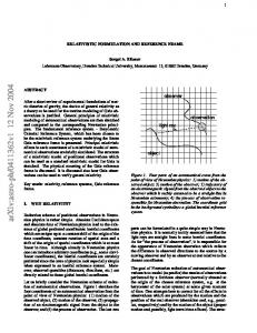
To order Ø(1/l) this is a rotational map around the axis (0, 1r csc θ cot γ2 , 1) through an angle ΩF (γ, θ) = q γ z sin r2 sin2 θ sin2 γ2 + cos2 γ2 , and in particular it is l 2 clear that liml→∞ ΩF (γ, θ) = 0. This rotational dynamics is illustrated in Fig. 2, where we perform repeated coherent interactions between the QRF and a stream of source particles.

6

1 t=π/2 t=π t=2π Sequential measurements

Probability of success

0.9

0.5

/l

0

−0.5

−1 1

t=π/2 t=π t=2π

0.8 0.7 0.6 0.5 0.4 0.3 0.2

1

0.5 /l

0 0

−1

0

100 200 300 400 500 Number of measurements or unitary interactions

/l

FIG. 2: hLx i/l, hLy i/l and hLz i/l. The rotation induced on the reference frame due to the unitary interaction with the source particle for l = 16. The source particles are polarized along the z-axis with z=1 and the QRF initially points along the x-axis, θ = π/2. In this figure N=500 source particles has been used.

CORRECTING THE DRIFT OF A QUANTUM REFERENCE FRAME

In this section we consider certain approaches that allow us to correct the drift of the reference frame due to the projective measurement {Π± }. If, in addition to the source of particles S, which are aligned in the Z-direction, we also have access to an¯ which are aligned in the −Zother set of particles S, direction, then our intuition is that we may recover the quadratic scaling of [12] by alternating the measurements on systems from S with measurements on systems from ¯ Since the sequence of measured particles has zero net S. polarization no directional drift of the QRF occurs. However, this approach requires the use of an equal number of ‘corrective’ S¯ particles as measured particles but is this the optimal strategy to eliminate drift? Two different strategies present themselves, but before discussing them we first establish an operational criterion for the usefulness of the QRF.

Operational Criterion

We wish to define an operational criterion by which to judge how well the finite-sized QRF does in the task of mimicking a projective measurement on the source particles.

FIG. 3: Psucc as a function of the number of interactions for the case in which source particles are polarized along the zaxis (z = 1) and the QRF is initially in the coherent state l = 16 pointing along the x-axis, i.e. θ = π/2.

To judge the quality of the measurement we follow [12] and consider the probability of successfully finding the correct result l + 21 when the test particle is pointing along +ˆ n (the initial direction of the reference frame)or finding the correct result l − 12 when the test particle is pointing along −ˆ n: 1 Tr[Π+ (ρ ⊗ |ˆ nihˆ n|) + Π− (ρ ⊗ | − n ˆ ih−ˆ n|)] 2 1 = (1 + n ˆ·n ˆ ρ ). (27) 2

Psucc =

In [12] it was shown that the number of measurements a QRF could be used for before Psucc falls below some threshold scaled quadratically with l if the source of particles was unpolarized. In [11] it was shown that the scaling becomes only linear with l if the source of particles being measured has some net polarization. In Fig. 3 we show the degradation of the reference frame under a sequence of either measurement interactions (solid line) or unitary interations for various values for γ. Correction via Unitary Interactions

The first corrective mechanism we consider is to make two measurements of particles from S and then to implement a unitary U = e−i2πL·S between the QRF and a ¯ particle from S. In Fig. 4 we plot the Z-component of angular momentum of the QRF versus its x-component. The blue line is the degradation with no correction, as considered in [11]. The red line is for the case in which we have applied the

7

1.2

1

1 Probability of success

0.9

/l

0.8 0.6 0.4 0.2 0 −0.2 0

0.8 0.7 0.6 0.5

0.2

0.4

0.6

0.8

0.4

1

/l

FIG. 4: hLz i/l vs. hLx i/l for l = 16. The source particles are polarized along the z-axis and the QRF is initially in the coherent state pointing along the x-axis. The blue dotted line corresponds to the case of sequential measurements and the red dotted line is for the case of unitary interaction ei2πL·S after two measurements.

unitary mentioned above after every two measurements we observe that this method helps us to essentially completely correct the rotation of QRF (the drift towards the polarization of S). To understand why this works, we see from equation (25) that the unitary interaction can generate a rotation 2 about the Y -axis of rz l sin θ sin γ/2. For the particular choice of γ = π we have that the unitary interaction produces a rotation exactly twice as large as the measurement interaction, while maintaining the reference frame in the X-Z plane. By using a source particle from S¯ we can ensure that this rotation acts in the opposite direction to the drift to equilibrium, and it is easily checked that Fπ [E 2 [ρ]] = ρ + Ø(1/l2 ).

(28)

An important point to emphasize is that the application of the unitary interaction not only can correct the polarization drift to Ø(1/l2 ), but it does so without requiring knowledge of the relative angle θ between the QRF and the source particles. For very large l we have greater freedom regarding when in the course of a sequence of N measurements the corrective unitaries are performed. If 1  N  l, then we have that p± (θ) is roughly constant over the course of N measurements. The actual measurement sequence is highly probable to be a typical measurement sequence with p+ N plus outcomes and p− N minus outcomes. However, since N  l the QRF has rotated through a total angle p+ N Ω+ + p− N Ω− = N Ω,

0

500

1000 1500 2000 Number of measurements

2500

FIG. 5: A comparison of probability of success for obtaining correct measurement result in three different cases for l = 16. The dashed line corresponds to the case of sequential measurements, the dashed-dotted line is for the case in which we correct the measurement result via applying unitary interactions after two measurements and the solid line belongs to the case of correction via applying unitary interactions after each plus outcome.

which may be corrected with N/2 unitary interactions distributed arbitrarily between the N measurements. In Fig. 5, Psucc is plotted against the number of measurements for the two cases mentioned above. We can clearly see that the longevity of the QRF is now improved. In this figure the horizontal axis is for the number of measurements and the particles used to improve the probability of success are not included, so with the use of particles from S¯ we may extend the lifetime of the QRF to Ø(1/l2 ) in a more efficient manner than described in the previous section.

Keeping track of measurement results

None of the work on QRF degradation has considered the option of keeping track of the measurement results. This has been primarily for the sake of maintaining a simple pedagogy. We can now consider the possibility of actively feeding back individual measurement results to correct the frame’s drift. With probability p+ the QRF is transformed as ρ → E+ [ρ] and similarly with probability p− the QRF is transformed as ρ → E− [ρ]. A measurement history for the reference frame may be described via ~s = (s1 , s2 , . . . , sN ), with si = ±. This sequence of outcomes in term corresponds to a evolution of the QRF given by E~s [ρ] := EsN [· · · Es2 [Es1 [ρ]]].

8 The probabilities for large l are given by p± (θ) = 12 (1± zr cos θ) where z is the polarization of the source particles and l is the polarization of the of the reference frame, as described earlier. Since we are considering Ø(1/l) effects we shall assume that r is approximately constant for N  l. Note that in the context of the above measurement history, the probabilities for each outcome si are not independent since p± has angular dependence and so depends on previous rotations induced by si−1 , si−2 , . . . . We may again use the unitary interaction, however unlike the case of the average map E, no simple correction exists for an individual plus or minus outcome for two reasons. Firstly, the angle of rotation generated by the unitary interaction decreases monotonically with l and so fluctuations, such as the ones discussed earlier, may be much too large to correct. Secondly, the unitary rotation goes sinusoidally with the relative angle θ between the source particles and the QRF, while the rotations due to the individual outcomes are in general complicated functions of θ. A knowledge of θ would be needed to tune the unitary interaction correctly. However, it should be that any auxilary background reference frame that we may introduce should not feature in the experimental considerations, and should serve only as a useful intermediate construct. ‘Information is physical’, and so any meanful coordinate system must be associated with an actual physical system. Of course, one could take the view that an large background system already exists, and relative to this we have already determined the angles of inclinations of both the source particles and quantum reference frame, and hence know the value for θ. However, in this case, the goal of considering unitary corrections would then be to preserve the known state of the QRF in between measurements, as distinct from providing a reliable reference frame with which one determines the unknown relative angle with an ensemble of source particles through repeated measurements. With a knowledge of the relative angle θ we may tune the unitary interaction appropriately, using either ¯ and correct sufficiently a source particle from S or S, small rotations of the QRF. However, in the event of large measurement rotations, the best we can do between individual measurements would be to perform the largest allowable rotation in the required direction - numerics indicate that for the two projective outcomes Π± we can always correct one outcome entirely and the other for π/2 < θ < π.

DISCUSSION AND OUTLOOK

In this paper we have analysed in some detail the induced dynamics of a quantum reference frame as it is used to measure the spins of a sequence of source parti-

cles, and also used to implement unitary interactions on the source particles. We found that the average behaviour of the QRF is to gradually rotate into alignment with the source particles at an Ø(1/l) rate. If we pay attention to the induced dynamics subsequent to a particular measurement outcome, we find that the dynamics is not so simple and large fluctuations can exist, which depend on observables quadratic in L. We considered the restriction to a simple class of initial states for which the dynamics depends purely on the inclination of the QRF relative to the source particles. For such states we found that fluctuations may persist even in the infinite limit, and which give non-trivial dynamics. Of course in this limit there is, on average, no net rotation of the QRF. We found that by performing a unitary interaction between the QRF and source particles every third step, we could eliminate the Ø(1/l) directional of the reference frame under the average map. Future work might include the issue of parameterestimation on the state of the source particles. While ordinary projective measurements possess a degeneracy between the polarization of the source particles and the relative angle between the QRF and the particles, the presence of dynamics breaks this degeneracy and potentially allows a richer measurement inference. In the ideal projective measurement case, the measurement probabilities are given by p± = (1/2)(1 ± z cos θ), and so doing a sequence of measurements only gives us the value of z cos θ. However, in the presence of dynamics, the reference frame responds differently to the polarization z of the source and to the relative angle θ with the source. For example, by allowing the QRF to gradually come into alignment with the source particles the measurement pattern is eventually determined solely by z, while the early-time outcomes encode the dependence on θ. Such a separation of parameters is a result of the nontrivial dynamics of the finite quantum reference frame. It is also possible to do parameter estimation plus correction in parallel. Initially we know nothing of θ and so can take it to lie uniformly between 0 and π. However, for example, getting a string of many plus outcomes implies that the relative angle θ is quite small. Each successive measurue outcome we obtain allows us to update our estimate for θ and in each case we can use our best estimate to perform a unitary correction, ideally converging in on a stable distribution and the correct value for the relative angle. Alternatively, in the event that we are ignorant of the relative angle θ it may be possible to perform a ‘conditional’ corrective unitary interaction. The idea is that the source particle that has been measured with the QRF encodes the relative angle between the QRF and the unmeasured particles in its new state. It may be possible to transfer this θ dependence to in a manner which improves the corrective procedures.

9 Finally, it would be of interest to extend the analysis we have conducted here to study how measurement and unitary interactions behave between a large QRF and higher spin particles.

[1] S. Bartlett, T. Rudolph, and R. Spekkens, Rev. Mod. Phys. 79, 555 (2007). [2] F. Costa, N. Harrigan, T. Rudolph, and C. Brukner, New J. Phys. 11, 123007 (2009). [3] S. Bartlett, T. Rudolph, R. Spekkens, and P. Turner, New J. Phys. 11 063013 (2009). [4] F. Costa, N. Harrigan, T. Rudolph, and C. Brukner, New J. Phys. 11, 123007 (2009). [5] Gambini, R., R. A. Porto, and J. Pullin, Phys. Rev. Lett. 93, 240401 (2004); ibid New J. Phys. 6, 45 (2004). [6] F. Girelli and D. Poulin, Phys. Rev. D 77 104012, (2008). [7] D. N. Page and W. K. Wootters, Phys. Rev. D 27, 2885 (1983)

[8] S. Bartlett, T. Rudolph, B. C. Sanders and P. Turner, J. Mod. Opt. 54 2211 (2007). [9] S. Bartlett, T. Rudolph, and R. Spekkens, Phys. Rev. A. 70, 032321 (2004). [10] J.-C. Boileau, L. Sheridan, M. Laforest, S. Bartlett, J. of Math. Phys. 49, 032105 (2008). [11] D. Poulin, and J. Yard, New. J. Phys. 9, 156 (2007). [12] S. Bartlett, T. Rudolph, R. Spekkens, and P. S. Turner New. J. Phys. 8, 58 (2006). [13] M. A. Nielsen and I. L. Chuang, Quantum Computation and Quantum Information, (Cambridge University Press, Cambridge, 2000). [14] M. E. Rose, Elementary Theory of Angular Momentum (Wiley, New York, 1957). [15] A. R. Edmonds, Angular Momentum in Quantum Mechanics (Princeton University, Princeton, New Jersey, 1957). [16] W. G. Ritter, J.Math. Phys. 46 082103 (2005). [17] S. J. van Enk, H. J. Kimble, Quantum Information & Computation, 2, 1 (2002)