dynamics of ion-scale coherent magnetic structures and coupling with

DYNAMICS OF ION-SCALE COHERENT MAGNETIC STRUCTURES AND COUPLING WITH WHISTLER WAVES DURING SUBSTORMS. Anna Tenerani

To cite this version: Anna Tenerani. DYNAMICS OF ION-SCALE COHERENT MAGNETIC STRUCTURES AND COUPLING WITH WHISTLER WAVES DURING SUBSTORMS.. Plasma Physics [physics.plasm-ph]. Université Pierre et Marie Curie - Paris VI, 2012. English.

HAL Id: tel-00789137 https://tel.archives-ouvertes.fr/tel-00789137 Submitted on 15 Feb 2013

HAL is a multi-disciplinary open access archive for the deposit and dissemination of scientific research documents, whether they are published or not. The documents may come from teaching and research institutions in France or abroad, or from public or private research centers.

L’archive ouverte pluridisciplinaire HAL, est destinée au dépôt et à la diffusion de documents scientifiques de niveau recherche, publiés ou non, émanant des établissements d’enseignement et de recherche fran¸cais ou étrangers, des laboratoires publics ou privés.

Thèse de doctorat en cotutelle entre Université Pierre et Marie Curie Ecole Doctorale "Astronomie et Astrophysique d’Ile de France" Università degli Studi di Pisa Dottorato di ricerca in Fisica Applicata

Anna Tenerani Dynamics of ion-scale coherent magnetic structures and coupling with whistler waves during substorms Soutenue le 26 octobre 2012 Jury:

P. Boissé L. Rezeau F. Califano O. Le Contel G. Zimbardo P. Louarn F. Pegoraro D. Del Sarto

Professeur UPMC Professeur UPMC Professeur Universitá di Pisa CR/CNRS Professeur Universitá della Calabria DR/CNRS Professeur Universitá di Pisa MdC Université de Lorraine

Président du jury Directrice de thèse Directeur de thèse Co-directeur de thèse Rapporteur Rapporteur Examinateur Examinateur

i

Ringraziamenti Desidero ringraziare il mio relatore italiano Prof. Francesco Califano e il mio co-relatore francese Dr. Olivier Le Contel per il loro aiuto e supporto nello svolgere questo lavoro. Soprattutto li ringrazio per avermi dato, assieme alla mia relatrice francese Prof.ssa Laurence Rezeau, l’opportunità di studiare al Laboratoire de Physique des Plasmas, a Parigi. Ringrazio il gruppo di plasmi di Pisa, che sicuramente è un riferimento fondamentale per me, ed in particolare ringrazio il Prof. Francesco Pegoraro per la sua disponibilità nel dare utili suggerimenti. Patrick Robert, che ha contribuito all’analisi dei dati sperimentali, ed è sempre pronto ad aiutarmi nell’uso dei programmi di analisi sperimentale. Il Prof. Marco Velli, che con pazienza mi ha dato consigli per migliorare la stesura di questo testo. Daniele Del Sarto, che è sempre disponibile e il cui appoggio è stato di grande aiuto durante quei momenti difficili che di certo non sono mancati in questi tre anni. Infine, ringrazio la mia famiglia e i miei genitori per il loro continuo sostegno ed incoraggiamento.

Parigi, 10 settembre 2012

A. T.

Remerciements J’ai grand plaisir à remercier mon directeur de thèse italien, le Professeur Francesco Califano, et mon co-directeur de thèse le Docteur Olivier Le Contel, pour l’aide et le support qu’ils m’ont fourni pour le développement de ce travail. Je tiens aussi à remercier ma directrice de thèse française le Professeur Laurence Rezeau, pour m’avoir donné la possibilité d’étudier au Laboratoire de Physique des Plasmas, à Paris. Je remercie également les membres du groupe de plasmas de Pise, pour tout ce qu’ils m’ont apporté aussi bien sur le plan scientifique que sur le plan humain. Je remercie en particulier le Professeur Francesco Pegoraro pour sa disponibilité et ses suggestions. Je souhaiterais aussi remercier Patrick Robert, qui a contribué à l’analyse des données et qui a toujours été prêt à m’aider avec les outils d’analyse expérimentale; le Prof. Marco Velli, qui m’a aidé avec patience à améliorer l’écriture de ce texte; Daniele Del Sarto, pour sa disponibilité et ses bons conseils et dont l’appui a été fondamental dans les moments difficiles qui n’ont pas manqué de survenir pendant ces trois années. Enfin, je remercie ma famille et mes parents pour leur soutien et leurs encouragements permanents.

Paris, le 10 septembre 2012

A. T.

ii

iii

Abstract A new model of the self-consistent coupling between low frequency, ion-scale coherent magnetic structures and high frequency whistler waves is proposed in order to interpret space data gathered by Cluster satellites during substorm events, in the night sector of the Earth’s magnetosphere. The coupling provides a mechanism to spatially confine and transport whistler waves by means of a highly oblique, propagating nonlinear carrier wave. The present study relies on a combination of data analysis of original in situ measurements, theoretical modeling and numerical investigation. During substorms, the magnetosphere undergoes strong magnetic and electric field fluctuations ranging from low frequencies, of the order or less than the typical ion-time scales, to higher frequencies, of the order or higher than the typical electron time-scales. To understand basic plasma physical processes which characterize the magnetosphere dynamics during substorms an analysis of whether, and by which mechanism, waves occurring at these different time scales are coupled, is of fundamental interest. Low frequency magnetic structures are commonly detected in environments such as the magnetosheath and the solar wind, as well as in the dusk magnetosphere, possibly correlated with higher frequency whistler waves. In this Thesis it is shown that similar magnetic structures, correlated with whistler waves, are observed in the magnetospheric plasma sheet during substorms. The interesting question arises as to how the inhomogeneity associated with such magnetic structures affects the propagation of higher frequency waves. The Cluster mission, thanks to its four satellites in tetrahedron configuration and high temporal resolution measurements, provides a unique opportunity on the one hand to explore the spatial structure of stationary and propagating perturbations observed at low frequencies and on the other hand to study dynamics occurring at higher temporal scales, via whistler mode waves. With regard to this, I will describe the Cluster spacecraft detection of large amplitude whistler wave packets inside coherent ion-scale magnetic structures embedded in a fast plasma flow during the August 17, 2003 substorm event. In this period the Cluster satellites were located in the plasma sheet region and separated by a distance which is less than the magnetotail typical ion-scale lengths, namely the ion gyroradius and the ion inertial length. The observed whistler emissions are correlated with magnetic field structures showing magnetic depletions associated with density humps. As a first step, the latter have been modeled as one dimensional nonlinear slow waves which spatially confine and transport whistlers, in the framework of a two-fluid approximation. This schematic model is investigated through a theoretical and numerical study by means of a two-fluid code, and it is shown that the proposed model goes quite well with data interpretation. Its possible role in substorm dynamics is also discussed. This new trapping mechanism, studied here by using a highly oblique slow magnetosonic soliton as a guide for whistler waves, is of more general interest beyond the specific context of the observations reported in this Thesis. Other nonlinear structures showing similar features, for example highly oblique nonlinear Alfvén waves or kinetic Alfvén waves in high beta plasmas, can in principle act as wave carriers. The model proposed provides an explanation for the recurrent detection of whistlers inside ion-scale magnetic structures which is alternative to usual models of stationary magnetic structures acting as channels. Moreover, the study described in this Thesis addresses more general questions of basic plasma physics, such as wave propagation in inhomogeneous plasmas and the interaction between wave modes at different temporal scales.

iv

v

Résumé Dans cette thèse, on propose un nouveau modèle de couplage auto-cohérent entre des structures magnétiques cohérentes sur les échelles ioniques et des ondes dites de sifflement (whistlers, en anglais) à plus hautes fréquences, afin d’interpréter les données expérimentales recueillies par les satellites Cluster pendant un sous-orage magnétique dans la région nocturne de la magnétosphère terrestre. Le couplage fournit un mécanisme pour confiner et transporter les ondes whistlers par l’intermédiaire d’une onde nonlinéaire qui se propage obliquement par rapport au champ magnétique. Cette étude s’appuie sur une analyse des données expérimentales, sur une modélisation théorique ainsi que sur des simulations numériques. Pendant les sous-orages magnétiques, la magnétosphère est soumise à de fortes perturbations magnétiques et électriques dans une vaste gamme de fréquences, qui vont des basses fréquences, inférieures ou de l’ordre de l’échelle temporelle typique ionique, aux hautes fréquences, supérieures ou de l’ordre de l’échelle temporelle typique électronique. Afin de connaître les processus physiques qui déterminent la dynamique de la magnétosphère pendant les sous-orages, il est fondamental de comprendre si, et avec quel méchanisme, des couplages peuvent se produire entre des ondes qui se propagent sur des temps caractéristiques différents. Des structures magnétiques à basse fréquence ont déjá été obsérvées dans des régions comme la magnétogaine et le vent solaire, éventuellement associées à des ondes whistlers à plus haute fréquence. Dans cette thèse, on montre que des structures similaires sont obsérvées dans la couche de plasma à l’intérieur de la magnétosphère. On s’interroge ensuite sur la façon dont l’inhomogénéité de telles structures peut influencer la propagation des ondes à plus haute fréquence. Grâce à ses quatre satellites en configuration tetraédrique et à ses mésures à haute résolution temporelle, la mission Cluster nous offre une occasion unique de pouvoir analyser la structure spatiale des perturbations stationnaires (ou se propageant) et d’étudier la dynamique du plasma sur des échelles temporelles plus courtes, telles que celles des ondes whistlers. Ainsi, je décrirai les émissions d’ondes whistlers détectées par les satellites Cluster à l’intérieur de structures magnétiques cohérentes situées dans un écoulement de plasma rapide pendant le sous-orage du 17 Août 2003. Au cours de cette période, les satellites Cluster sont situés dans la couche de plasma, séparés d’une distance de l’ordre des échelles spatiales typiques ioniques (le rayon de giration ou la longueur d’inertie des ions). Les ondes whistlers sont corrélées avec des structures magnétiques charactérisées par un minimum du module du champ magnétique et un maximum de densité du plasma. Ces dernières ont été modélisées comme des ondes planes nonlinéaires de type lent qui piègent et transportent les ondes whistlers. A partir d’une étude théorique et numérique en utilisant une approche bi-fluide, on peut alors reproduire les données observationnelles. Le rôle possible de telles structures couplées dans la physique des sous-orages est aussi discuté. Ce nouveau mécanisme de piégeage, étudié ici en utilisant comme guide pour les whistlers une onde oblique de type magnétosonique, est d’intérêt plus général par rapport au contexte spécifique des observations présentées dans cette thèse. En effet, d’autres ondes nonlinéaires, comme par exemple les ondes d’Alfvén obliques ou d’Alfvén cinétiques dans les plasmas à beta fort (où beta est le rapport de la pression thermique du plasma sur la pression magnétique), pourraient aussi transporter les whistlers. Ce modèle de piégeage constitue aussi une explication alternative aux modèles existants qui considèrent une inhomogénéité stationnaire sous la forme d’un canal de densité. Enfin, l’étude décrite dans cette thèse concerne des problématiques fondamentales en physique des plasmas, comme la propagation d’ondes dans les milieux inhomogènes et l’interaction entre modes sur des échelles temporelles différentes.

vi

vii

Riassunto In questa Tesi viene proposto un nuovo modello di accoppiamento auto-consistente tra strutture magnetiche coerenti sulle scale ioniche e le cosiddette onde whistlers a piú alta frequenza, al fine di interpretare dati sperimentali raccolti dai satelliti Cluster durante una sotto-tempesta magnetica nella regione notturna della magnetosfera terrestre. L’accoppiamento fornisce un meccanismo per confinare spazialmente e trasportare onde whistlers tramite un’onda nonlineare che si propaga obliquamente rispetto al campo magnetico. Questo studio si basa su un’ analisi originale di dati sperimentali, modellizzazione teorica e indagine numerica. Durante le sotto-tempeste magnetiche, la magnetosfera è soggetta a forti fluttuazioni magnetiche ed elettriche in una vasta gamma di frequenze, da quelle dell’ordine o inferiori alla tipica scala temporale ionica, alle alte, dell’ordine o maggiori della tipica scala temporale elettronica. Per conoscere i processi fisici di base che determinano la dinamica della magnetosfera durante le sotto-tempeste magnetiche, è fondamentale capire se, e con quale meccanismo, si possono accoppiare onde che si propagano su tempi scala diversi. Strutture magnetiche a bassa frequenza sono osservate comunemente in regioni come la magnetoguaina e il vento solare, eventualmente associate alle onde whistlers. In questa Tesi viene mostrato che simili strutture sono osservate nello strato di plasma all’interno della magnetosfera terrestre. Si pone quindi l’interessante problema su come la disomogeneità di tali strutture influenzi la propagazione di onde a piú alta frequenza. La missione Cluster, grazie ai suoi quattro satelliti in configurazione tetraedrica e alle misure ad alta risoluzione temporale, offre un’ occasione unica, da un lato per analizzare la struttura spaziale di perturbazioni stazionarie o che si propagano, dall’altro di studiare la dinamica mediata dai whistlers su scale temporali piú rapide. A questo proposito descriveró le misure di onde whistlers effettuate dai satelliti Cluster all’ interno di strutture magnetiche coerenti immerse in un flusso di plasma rapido, durante la sottotempesta magnetica del 17 Agosto 2003. In quel periodo i satelliti Cluster erano localizzati all’interno dello strato di plasma nella regione notturna della magnetosfera, separati da una distanza dell’ordine delle tipiche scale spaziali ioniche, il raggio di Larmor e la lunghezza inerziale ionica. Le onde whistlers osservate sono correlate con strutture coerenti caratterizzate da un minimo del modulo del campo magnetico e un massimo della densità del plasma. In prima approssimazione, queste ultime sono state modellizzate come onde piane nonlineari di tipo lento che intrappolano e trasportano le onde whistlers in un plasma a due fluidi. Questo modello viene approfondito attraverso uno studio teorico e numerico con un codice a due fluidi, e viene mostrato che risulta adeguato all’interpretazione dei dati osservativi. Viene discusso anche il possibile ruolo di tali strutture accoppiate nella dinamica delle sotto-tempeste magnetiche. Il nuovo meccanismo di intrappolamento proposto in questa Tesi, studiato usando un’onda obliqua di tipo magnetosonico come guida per i whistlers, è di interesse piú generale rispetto allo specifico contesto dato dalle osservazioni riportate in questa Tesi. Altre onde nonlineari, come per esempio le onde oblique di Alfvén o le onde di Alfvén cinetiche in plasmi ad alto parametro beta, possono agire come mezzo per trasportare i whistlers. Il modello proposto fornisce anche una spiegazione per le ricorrenti osservazioni di whistlers all’interno di strutture magnetiche alle scale ioniche, che è alternativa rispetto agli usuali modelli in cui la disomogeneità stazionaria agisce come canale. Inoltre, lo studio descritto in questa Tesi è rivolto a problematiche di fisica del plasma di base, come la propagazione di onde in mezzi disomogenei e l’interazione tra modi su scale temporali diverse.

viii

ix

Contents Abstract

ii

Résumé

iv

Riassunto

vi

1 Introduction 2 Theoretical Background 2.1 Whistler waves . . . . . . . . . . . . . . . . . . . . . . . 2.1.1 Whistler mode in the cold plasma approximation 2.1.1.1 Propagation in a homogeneous medium 2.1.1.2 Propagation in density inhomogeneities. 2.1.2 Effect of temperature and the whistler anisotropy 2.2 Slow magnetosonic solitons . . . . . . . . . . . . . . . .

1

. . . . . . . . . . . . . . . . . . . . . . . . . . . . . . . . . Geometrical optics instability . . . . . . . . . . . . . . . .

3 Observations: the substorm event on August 17, 2003 3.1 Data and instrumentation . . . . . . . . . . . . . . . . . . . . . . . 3.2 Overview of the event . . . . . . . . . . . . . . . . . . . . . . . . . 3.3 Whistler wave analysis . . . . . . . . . . . . . . . . . . . . . . . . . 3.3.1 Whistler wave detection inside coherent ion-scale structures 3.3.1.1 Case 1 . . . . . . . . . . . . . . . . . . . . . . . . . 3.3.1.2 Case 2 . . . . . . . . . . . . . . . . . . . . . . . . . 3.3.1.3 Case 3 . . . . . . . . . . . . . . . . . . . . . . . . . 3.3.1.4 Summary . . . . . . . . . . . . . . . . . . . . . . . 3.4 Discussion . . . . . . . . . . . . . . . . . . . . . . . . . . . . . . . .

. . . . . . . . .

. . . . . . . . .

. . . . . . . . .

. . . . . . . . .

. . . . . . . . .

. . . . . .

. . . . . . . . .

. . . . . .

. . . . . . . . .

. . . . . .

7 7 7 7 9 11 12

. . . . . . . . .

17 18 19 22 25 27 32 36 39 64

4 Theoretical model for whistler ducted propagation by ion-scale slow solitary waves 4.1 Model equations . . . . . . . . . . . . . . . . . . . . . . . . . . . . . . . . . . . . 4.1.1 Numerical model . . . . . . . . . . . . . . . . . . . . . . . . . . . . . . . . 4.2 Analytical study of whistler wave trapping by magnetic and plasma density inhomogeneities . . . . . . . . . . . . . . . . . . . . . . . . . . . . . . . . . . . . . . . 4.3 Numerical study of whistler trapping by slow magnetosonic solitons . . . . . . . . 4.3.1 Initial conditions . . . . . . . . . . . . . . . . . . . . . . . . . . . . . . . .

71 72 72 73 76 77

x

CONTENTS

4.3.2 4.3.3

4.3.1.1 Test of the slow soliton stability . . . 4.3.1.2 Mechanism of whistler wave injection Parameters of the simulations . . . . . . . . . . Numerical results . . . . . . . . . . . . . . . . .

. . . .

. . . .

. . . .

. . . .

. . . .

. . . .

. . . .

. . . .

. . . .

. . . .

. . . .

. . . .

. . . .

. . . .

. . . .

77 78 81 81

5 Discussions and conclusions

85

A Dispersion relation of a two fluid plasma

87

B Numerical scheme

91

C Whistler propagation in an inhomogeneous plasma. WKB

93

D Analytical solution of slow magnetosonic solitons

97

E STAFF-SA spectra

99

F Data Reduction F.1 Electric field . . . . . . . . . F.2 Spacecraft potential . . . . F.3 STAFF-SC . . . . . . . . . F.4 Current density calculation

. . . .

. . . .

. . . .

. . . .

. . . .

. . . .

. . . .

. . . .

. . . .

. . . .

. . . .

. . . .

. . . .

. . . .

. . . .

. . . .

. . . .

. . . .

. . . .

. . . .

. . . .

. . . .

. . . .

. . . .

. . . .

. . . .

. . . .

. . . .

. . . .

. . . .

103 103 103 104 104

G Analysis methods for spacecraft data 107 G.1 Polarization analysis for whistler waves . . . . . . . . . . . . . . . . . . . . . . . . 107 G.2 Minimum Variance Analysis . . . . . . . . . . . . . . . . . . . . . . . . . . . . . . 107 G.3 Multi spacecraft analysis of magnetic discontinuities . . . . . . . . . . . . . . . . 108 H Acronyms

111

Bibliography

113

1

Chapter 1

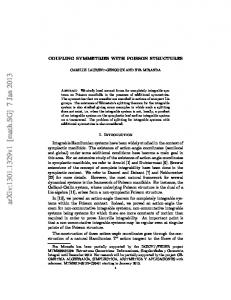
Introduction In this Thesis I present my research work which has focused on the interaction between whistler waves and nonlinear electromagnetic structures at the ion-scales in the plasma of the Earth’s magnetosphere. This work comprises an observational study based on data gathered in the night sector of the Earth’s magnetosphere by the Cluster spacecraft during a substorm event as well as a theoretical modeling of these observations, supported by numerical simulations involving a two-fluid model of the plasma. This work aims at investigating the spatial structure of low frequency fluctuations, namely at the typical ion-time scales by directly exploiting the unique multipoint capabilities and high time resolution measurements of the Cluster mission. It is found that such spatial structures can act as carriers for the higher frequency whistler waves during substorms. During substorm expansion Cluster detects, as shown both in the literature and in the following chapters, strong electric and magnetic field fluctuations ranging from low frequencies, of the order or less than the typical ion-time scales, to high frequencies, of the order or higher than the typical electron-time scales. An intrinsic property of plasmas is that once they have undergone some perturbation, they self-organize and exhibit collective motions coupled to electric and magnetic field fluctuations in the form of waves. In addition, in weakly collisional plasmas such as the magnetosphere, waves represent a fundamental way not only to transport information through the plasma, but also to mediate dynamics between particles. For this reason, the study of plasma wave modes and the interaction between waves occurring at different time scales is fundamental in order to understand magnetosphere dynamics and processes coming into play during substorms. In this sense, the four satellites of the Cluster mission, thanks to multipoint and high time resolution measurements, offer a unique opportunity to inspect the spatial structure of stationary and propagating magnetic fluctuations at low frequencies, and weather they are related to higher frequency waves. The present Thesis provides an investigation of the self consistent interaction between whistler mode waves and slow mode solitary waves by means of a combined study of observations, theoretical modeling and numerical investigation. The very existence of the magnetosphere is due to the continuous interaction of the Earth’s intrinsic dipolar magnetic field with the supersonic and superalfvénic streaming solar wind which drags the Interplanetary Magnetic Field (IMF) [1]. As shown in Fig. 1.1, the impinging solar wind compresses the Earth’s magnetic field on the dayside of the magnetosphere while on the nightside it stretches magnetic field lines outwards in a cometary tail-like configuration extending up to a few hundred Earth radii in the anti-sunward direction. The magnetospheric environment, as illustrated in Fig. 1.1, is structured in various regions. In this Thesis I investigate plasma dynamics occurring in the nightside magnetosphere, the magnetotail, where magnetic substorm

2

1. Introduction

B o w s h o c k

p a u s e

T a il lo b e P o la r c u s p

R o ta tio n a x is

S o la r w in d

P la s m a s p h e r e R a d ia tio n b e lt a n d r in g c u r r e n t

P la s m a s h e e t

m a g n e tic a x is

T a il lo b e

M

a g

ne to sh e a th

Figure 1.1: Schematic representation of the near Earth’s magnetosphere.

onset and expansion take place. The stretched configuration of the magnetotail is supported by an electric current across the tail, the central current sheet, also known as the cross-tail current. The latter is directed dawn-to-dusk and has a nominal value Jy = 1 − 4 nA/m2 during quiet periods [2, 3, 4], while during geomagnetic activity, as discussed below and in Chapter 3, it becomes more intense, reaching values of about 20−40 nA/m2 at the end of the substorm growth phase. The current sheet is about 2 − 5 Earth radii thick during quiet periods and it becomes thinner during substorms, with a thickness of about 0.2 − 1 Earth radii [2, 3, 4]. The central current sheet separates the magnetic field lines pointing Earthward in the northern hemisphere from those pointing tailward in the southern hemisphere. The lobes are the two regions of tenuous plasma which surround the denser and warmer central plasma sheet. In the lobes the plasma has an extremely low density, n ∼ 0.01 cm−3 , and electron and ion temperatures are Te ∼ 50 eV and Ti ∼ 150 eV [5], respectively, suggesting that field lines in this region are connected to the solar wind, allowing ions and electrons to flow away. The plasma sheet is typically 10 − 15 Earth radii thick and it carries part of the cross-tail current. In this region the plasma density is nearly n ∼ 0.1 − 1 cm−3 and temperatures are Te ∼ 0.6 keV and Ti ∼ 4 keV [5]. The plasma beta β, which is defined as the ratio between the thermal plasma pressure and the magnetic pressure, is of order unity since the magnetic field is relatively weak, especially in the field-reversal region (the so-called magnetic equator). The magnetic field lines of the plasma sheet connect to the auroral ovals (Fig. 1.2) where diffuse auroral precipitations take place in a quasi stationary regime, in addition to the brighter discrete auroral displays enhanced during highly magnetically disturbed periods. Finally, the plasma sheet is separated from the tail lobes by the plasma sheet boundary layer, where field aligned currents and plasma flows toward and away from Earth are often detected. The magnetosphere is dynamic, as it is continuously exposed to the variable conditions in the solar wind. The magnetosphere as described above, and represented in Fig. 1.1, can be considered the typical configuration reached by the Earth-solar wind system during quiet periods. Under particular conditions of the IMF, namely when it turns southward, the magnetosphere can undergo strong perturbations leading to a reconfiguration of the magnetic field and a redistribution of magnetic and particle energy, the magnetospheric substorms. A magnetospheric substorm is “a transient process initiated on the nightside of the Earth in which

1. Introduction

3

a significant amount of the energy derived from the solar wind-magnetosphere interaction is deposited in the auroral ionosphere and in the magnetosphere” (Rostoker et al., JGR (1980) [6]). The substorm process can be divided into three main phases: a growth phase, an expansion phase and a recovery phase. The growth phase [7] is the first stage of the substorm dynamics and typically starts after the IMF has turned southward allowing magnetic field lines to merge at the dayside boundary of the magnetosphere. The reconnected magnetic field lines then are dragged downstream of the Earth where they start to pile up. During the growth phase, which lasts about 0.5–1 hour, energy is stored in the magnetospheric nightside as the central current sheet intensifies and thins in the near-Earth plasma sheet region, extending all the way down to the geosynchronous orbit [8]. At the same time the auroral oval is seen to move equatorward [9] as the magnetic field lines are stretching in the tail, and the most equatorward auroral arc is seen to brighten as a consequence of the enhanced field aligned currents. Once the stored energy reaches a critical level, a local current instability is triggered (substorm onset) which leads to the disruption of the central current sheet. Energy is then rapidly released to the plasma sheet during the expansion phase, where particles are heated, accelerated and injected both Earthward, in the inner magnetosphere, and tailward [10]. Both ground based and in situ measurements reveal strong electromagnetic field fluctuations in a wide range of frequencies. With the disruption of the central current, the previously stretched magnetic field recovers a more dipolar-like configuration, a process called dipolarization. The most direct, and perhaps fascinating, evidence of substorm expansion are discrete auroras, or auroral substorms [9]. These are temporary brightenings in visible light, typically from red to green, that can be observed in the sky at high latitudes. Auroral displays appear at or near the substorm onset in the midnight sector and then they propagate westward and poleward. Discrete auroras are due to plasma sheet particle acceleration along the magnetic field lines connecting to the auroral oval. If electrons are sufficiently energetic to overcome the repulsive mirror force due to converging magnetic field lines toward the ionosphere, they fall into the ionosphere itself where they are lost through collisions with neutral atoms. After the expansion phase, which typically lasts 1 hour, the system recovers its pre-substorm state (recovery phase). The primary origin of the substorm onset is still a matter of debate. Two major paradigms have been proposed, Figure 1.2: Auroral oval. known as the near-tail initiation and the mid-tail initiation paradigms. A detailed review of the pros and cons of these two scenarios is beyond the scope of the present Thesis, and can be found for instance in the review paper by Lui (2004) [11]. For the sake of completeness, I only briefly summarize here the main features of the proposed scenarios. In the near-Earth initiation paradigm, a current disruption which could be provided by, e.g., ballooning modes or the cross-field current instability, is thought to take place in the near Earth region, between 6 and 15 Earth radii down in the tail. The local dipolarization enhances Earthward convection and the whole disturbance propagates tailward, in order to explain the poleward movement of the auroral arcs, as mentioned above. Magnetic reconnection at the magnetic equator can eventually occur as a result of a secondary instability. On the contrary, the mid-tail initiation paradigm relies on the hypothesis that magnetic reconnection is the primary origin of the onset mechanism, taking place at a radial distance between 15 and 30 Earth radii. The plasma outflow piles up in the near Earth region, where the dipolar field brakes the flow which in turn deviates to form a dusk-to-dawn current, yielding local dipolarization.

4

1. Introduction

While the gross features of this process of energy storage and release rely on consolidated and widely recognized signatures in the ionosphere and magnetosphere, the nature of the microscopic processes related to substorm onset and expansion, and how they are related, is still not completely understood. With regard to this, whatever substorm onset mechanism is considered, it is crucial to understand plasma wave mode dynamics inside the magnetosphere. Since the plasma in the magnetosphere is low collisional, waves play indeed a crucial role in the dissipation processes needed to convert magnetic energy into thermal and kinetic energy through wave-particle interactions or, vice-versa, to provide a means to absorb and transport plasma energy. In this work I will focus mainly on whistler waves. Whistler waves are electromagnetic waves propagating in a magnetized plasma at frequencies fci < f fce , fci and fce being the ion and electron cyclotron frequencies, respectively. The interest in understanding the origin and propagation of whistler waves stems from the fact that the electron scattering by whistler waves causes electron pitch angle diffusion into the loss cone and the subsequent enhancement of precipitations into the ionosphere [12]. Moreover, whistlers may affect the development of large scale instabilities, such as the tearing instability [13], by controlling the level of electron temperature anisotropy. Earlier observations of wave activity in the night sector of the magnetosphere reported sporadic emissions in the whistler frequency range, f = 10−300 Hz, and amplitudes of about 0.01−0.1 nT , while spacecraft were crossing the plasma sheet. These emissions were recorded both in the near magnetotail regions, at radial distances ranging from 10 to 35 Earth radii [14, 15, 16, 17] and in the distant tail, at radial distances between 100 and 210 Earth radii [17]. It was suggested that whistlers were more likely excited by electron beams in the regions near the boundary of the plasma sheet. These observations showed that whistlers can be commonly detected in the plasma sheet, but did not show how they could be related to substorm activity. More recently whistler observations have been related directly to processes occurring during substorms at radial distances of 10-15 Earth radii in the plasma sheet, such as local dipolarization [18] or plasma jet braking at flux pile-up regions [19]. In both cases, electrons respond adiabatically to variations of the magnetic field by developing a temperature anisotropy in their distribution function, enabling whistler waves to grow [20]. Whistlers have been also correlated with reconnection events as they were detected just prior and after the detection of a southward turning of the Bz component of the magnetic field associated to a tailward ion fast flow [21]. It has been also suggested that whistlers may be used as proxy for magnetic reconnection on the dayside of the magnetopause [22]. In addition to observations related to substorms, it is worth mentioning that in situ space measurements reported quasi monochromatic whistler waves in the frequency range f ≈ 0.1 − 0.2 fce , the lion roars, inside magnetic field depressions associated with density humps whose typical scale length is of the order of the ion-scales, so-called magnetic holes. The latter are usually interpreted as non-propagating mirror mode structures and have been detected in the Earth’s magnetosheath and in the dusk magnetosphere [23, 24, 25, 26, 27]. Mirror modes are the final stage of the ion mirror instability, so that they need proper environmental conditions in order to develop [28, 29]. On the other hand, other nonlinear structures can naturally arise in a weakly collisional, magnetized plasma characterized by a magnetic field depletion in opposition of phase with a density inhomogeneity, as discussed for instance by Bäumgartell, JGR (1999) [30] or Stasiewicz, PRL (2004) [31] with regard to magnetic structures observed in the magnetosheath and solar wind. Theoretical models of such structures are provided by, e.g., highly oblique Alfvén solitary waves and slow magnetosonic solitons in high beta plasmas [32, 33, 30, 34, 35]. If the whistler waves become trapped inside such structures, the problem arises as to how low frequency nonlinear modes can act as carriers for higher frequency waves. Indeed, as will be discussed in Chapter 2, a known property of whistlers is that in the presence of field aligned tubes of plasma

1. Introduction

5

density inhomogeneities, or density ducts, their energy can be guided for long times without spreading [36, 37, 38, 39]. Examples of such ducted propagation have been found using satellite observations in the near Earth magnetosphere [40, 41, 42] and also in laboratory plasmas [43]. Throughout this Thesis I will discuss new aspects of whistler wave generation and propagation by investigating the linear coupling of whistlers with quasi perpendicular, “slow” electromagnetic waves at the ion-scales. In this sense the Cluster mission, by combining high time resolution and multipoint measurements, is very well suited, allowing the detailed investigation of the interaction between wave modes occurring at different time scales, as well as identifying propagating or stationary spatial structures at the inter-satellite distance. In this work I report observations of intense, broad band whistler emissions, with amplitudes of about 0.5 − 0.8 nT and in the frequency range f ≈ 0.1 − 0.4 fce , correlated to magnetic field strength depressions associated with density humps, embedded in a fast ion flow. A new model for the self-consistent coupling between low frequency, ion-scale coherent structures with high frequency whistler waves is presented, providing a natural interpretation of the Cluster data. The idea relies on the possibility of trapping whistler waves by inhomogeneous external fields, where the whistlers can be spatially confined and propagate for times much longer than their characteristic electronic time scale. As a first step, I will take the example of a slow magnetosonic soliton acting as a wave guide in analogy with the ducting properties of an inhomogeneous plasma. The soliton is characterized by a magnetic dip and density hump that traps and advects high frequency waves on many ion times. In addition, observations show that inside such low frequency magnetic structures favorable conditions for whistler wave growth set in, namely an electron temperature anisotropy develops. In this way, the magnetic structures provide a mechanism for both whistler mode wave generation and transport. A possible role of this mechanism in the substorm process is also discussed. Besides the possible application to substorms, the present work addresses fundamental questions of basic plasma physics, namely the interaction between wave modes at different time scales and the associated wave energy transport, as well as wave propagation in inhomogeneous plasmas. Finally, the trapping mechanism proposed provides an explanation to the recurrent detection of whistler waves inside magnetic holes alternative with respect to stationary inhomogeneities acting as channels for whistler. The Thesis is organized as follows: in Chapter 2 I summarize the known theory of whistlers and slow magnetosonic solitons that are at the base of the present work; in Chapter 3 I will report a detailed analysis of the observation of whistler waves inside ion-scale magnetic structures during the August 17, 2003 substorm event; in Chapter 4 I report the theoretical and numerical analysis carried out to model observations and finally, in Chapter 5 the concluding discussion.

6

1. Introduction

7

Chapter 2

Theoretical Background This chapter reviews the main plasma dynamics relevant to the present research. As explained in the Introduction, throughout the Thesis I will discuss the linear coupling between whistler mode waves and magnetic structures at the ion-scales, that will be modeled as a high frequency solitary wave arising from the MHD slow mode branch. In order to facilitate the reading of the following chapters, I will summarize the basics of whistler wave theory and of nonlinear magnetohydrodynamic solutions of the slow mode. This chapter is organized as follows: in Section 2.1 I will consider dynamics occurring at typical frequencies ωci ω < ωce , where ωci and ωce are the electron and the ion cyclotron frequency, respectively, focusing on whistler wave properties; in Section 2.2 I will consider dynamics occurring at the ion scales, that is at typical time scales of the order or less than the ion cyclotron frequency ω . ωci , showing how magnetosonic solitary waves arise as solutions of a two-fluid system.

2.1

Whistler waves

In this section I summarize whistler wave properties within both the fluid (§2.1.1) and the kinetic (§2.1.2) formalism. Fluid equations are obtained in the cold plasma approximation, vth,e vph , where vth,e and vph are the electron thermal velocity and the whistler phase velocity, respectively. Even if this condition is not always fulfilled in space plasmas, it greatly simplifies equations and allows to provide a good description of the main characteristics of whistler waves. Nevertheless, there are effects due to the thermal motion of electrons that have to be dealt with a kinetic approach. In particular, by using the kinetic equations, I will review a particular type of microscopic instability, the whistler temperature anisotropy instability due to a bi-maxwellian equilibrium distribution function. This instability is relevant for us because it provides a source for whistlers, as will be discussed in the section about data analysis.

2.1.1 2.1.1.1

Whistler mode in the cold plasma approximation Propagation in a homogeneous medium

Whistlers can be obtained in a simple way as normal modes of the Electron-Magneto-HydroDynamics model (EMHD hereafter). The EMHD is a one fluid model which is suited for describing plasma dynamics at frequencies ω > ωci . In particular, we assume that frequencies satisfy ωci ω < ωce ωpe , where ωpe = 4πn0 e2 /me is the plasma frequency. In this condition a useful simplification is to neglect the dynamics of ions, which can be considered as a neutralizing background. Moreover, since ω ωpe we can assume quasi neutrality and neglect the displacement

8

2. Theoretical Background

current in Maxwell’s equations. All these assumptions yield the following EMHD equations: e ∂ue e E− + (ue · ∇)ue = − ue × B ∂t me me c

(2.1a)

4π neue (2.1b) c 1 ∂B ∇×E=− . (2.1c) c ∂t In the above equations, B and E are the magnetic and electric fields, respectively, ue is the electron fluid velocity and n is the plasma particle density. Consider now an homogeneous magnetized plasma at rest with an equilibrium magnetic field B0 directed along the z direction and density n0 . The set of equations (2.1) can be arranged by taking the curl of equation (2.1a), and combining it with Maxwell’s equations (2.1b)–(2.1c), as to obtain the induction equation 1 e d2e 1 ∂ 2 2 ∇ − 2 B+ (2.2) ∇ × (∇ × B) × ∇ − 2 B = 0, ∂t de me c de ∇×B=−

2 is the electron inertial length. Assume now perturbations to the equilibrium where d2e = c2 /ωpe of the form A exp(ik · r − iωt), where k = (kx , 0, kz ) ≡ (k⊥ , 0, kk ) is the wave vector. The propagation angle θ with respect to B0 is θ = arctan k⊥ /kk . Linearization of equation (2.2) around the equilibrium gives the following equation for the magnetic field perturbation b me c 1 2 i ω k + 2 b = −(B0 · k)(k × b), (2.3) e de

which yields the whistler dispersion relation ω = ωce

kk kd2e , 1 + d2e k 2

(2.4)

where ωce = eB0 /(me c) is the electron cyclotron frequency. The components of the magnetic and electric field, b and e, respectively, of the corresponding eigenvectors are by i bz , = = − tan θ bx cos θ by ey ω/ωce cos θ − 1 ez sin θ =i , = . ex ω/ωce − cos θ ex ω/ωce − cos θ

(2.5a) (2.5b)

From the expressions in the set of equations (2.5) we infer that for a generic propagation angle θ whistlers are elliptically, right handed polarized with respect to the direction of B0 , while they are circularly polarized with respect to the direction of the wave vector. The maximum propagation angle is θm = arccos(ω/ωce ). Above this value the wave is evanescent. The plot of the normalized frequency ω/ωce as a function of the normalized wave vector kde is shown in Fig. 2.1, right panel, for different propagation angles. For future convenience, in Fig. 2.1, middle and right panels, I show the shaded isocontours of the normalized frequency ω/ωce , given by equation (2.4), in the plane (k⊥ , kk ). These contour plots are also known as refractive-index surfaces, shown, for the sake of illustration, only for positive values of kk and k⊥ . The surfaces can be obtained in the whole domain of wave vectors by tilting the plot with respect to the k⊥ axis and rotating around the kk axis. The shaded isocontours of the frequency are represented for values in the range

9

2.1. Whistler waves

ω/ωce < 1/2 and ω/ωce > 1/2, in left and right hand panels, respectively. Fig. 2.1 shows that at fixed frequency and kk there are two values, or two branches, for the perpendicular wave vector k⊥ , indicated as k− and k+ , respectively. For frequencies ω/ωce < 1/2 the two branches coexist, k− corresponding to a smaller angle of propagation with respect to k+ , while for frequencies ω/ωce > 0.5 only k+ can propagate. 1.0

0.3 CosΘ

0.25 0.2

0.6

k

Θ = 50 °

4

k

Θ = 34 °

6

Ω > 0.5 Ωce

20

0.35

Θ=0

0.8

Ω Ωce

Ω < 0.5 Ωce

8

0.15

0.4

0.7 0.65

18

0.6

16

0.55

14 12

0.1

2

0.2 0.0 0

2

4

6 k de

8

10

0 0

k5

8

k+ 10 k¦

15

0.4

10 0.5

0.05 20

0

5

k+ 10 k¦

15

20

Figure 2.1: Whistler dispersion relation. Left Panel: whistler dispersion relation (2.4) as a function of the modulus of the wave vector k for three different propagation angle θ. Middle and right panels: shaded isocontours for the whistler frequency ω/ωce given by equation (2.4), in k space. Middle and right hand panels correspond to the frequency regime ω/ωce < 1/2 and ω/ωce > 1/2, respectively.

2.1.1.2

Propagation in density inhomogeneities. Geometrical optics

The geometrical optics, or ray tracing theory, describes the propagation of electromagnetic wave packets in an inhomogeneous medium in terms light ray paths. This formalism is valid in the limit of small wavelengths with respect to the scale length of variation of the equilibrium quantities. In the following, the equations describing ray paths are derived in the simplified case of an isotropic medium (references can be found for instance in the textbooks “The Classical Theory of Fields” by Landau [44] §7, or “Principles of Optics” by Born and Wolf [45] §3). A detailed calculation for the case of whistlers in a magnetized plasma is presented in Appendix C. Let me consider for simplicity an isotropic, inhomogeneous medium whose properties vary over a typical scale length L, and consider time harmonic perturbations of the equilibrium of the form A(r/L)eik0 LS(r/L) e−iωt .

(2.6)

In equation (2.6), k0 = ω/c is the vacuum wave vector that satisfies k0 L 1. The phase S(r/L) and the amplitude A(r/L) are slowly varying functions of the position r, with respect to the wavelength. According to these assumptions, the set of Maxwell’s equations can be reduced to the wave equation ∇2 E + k02 ε(r, ω)E = 0,

(2.7)

where ε(r, ω) is the local dielectric response of the medium, and spatial lengths have been normalized to L. Since the dielectric function is a scalar, hereafter we can focus our attention to only one scalar component of the electric field. By inserting the explicit spatial form of the field E(r) = A(r)eik0 S(r) into the wave equation (2.7), we get the following expression ∇2 A − k02 (∇S)2 A + 2ik0 ∇A · ∇S + iAk0 ∇2 S + k02 εA = 0,

(2.8)

that can be solved, according to the WKB method, by expanding the amplitude A and the phase S in powers of k0−1 : A = A0 + k0−1 A1 + . . . , S = S0 + k0−1 S1 + . . . . If only the leading terms are

10


retained in equation (2.8), the phase of the wave is described by the so called eikonal equation (∇S0 )2 = ε, or [∇ (k0 S0 )]2 = k 2 , (2.9) n h R p io r ∇S0 0 − ωt ε(r0 ) |∇S · dr which yields E(r, t) = E0 exp i k0 . This solution corresponds 0| to the geometrical optics approximation. Remark that the amplitude of the wave varies slower than the phase k0 S. As a consequence, the first corrections in the amplitude p are due to terms −1 proportional to ∼ k0 in equation (2.8), which yield an amplitude A0 = 1/2 ε(r). In summary, in the small wavelength limit k0 L 1 waves propagating in an inhomogeneous medium can be described by the form eiφ , where φ = k0 S0 − ωt. The frequency is ω = ∂φ/∂t and the wave vector k = ∇φ is locally orthogonal to the surfaces of constant phase. These equations are analogous to those of a classical particle, the wave vector k and the frequency ω of the wave playing the role of the momentum p and the Hamiltonian H of the particle, respectively. By analogy, wave packets propagate along ray-paths r(t) of constant phase φ, at the group velocity r˙ = ∂ω/∂k. The equation describing the time evolution of the ray path is given by the solution of the Hamiltonian system ∂ω ∂ω ˙ = −k(t), = r˙ (t). (2.10) ∂r ∂k In support of the analysis carried out in Section 4.2, it is useful to briefly describe here the propagation of whistlers in field aligned density enhancements or depletions, the so called density ducts, in the geometrical optics approximation, highlighting the basic mechanism of whistler trapping. Whistler propagation in density ducts was first studied by Smith and Helliwell by using the ray tracing technique in order to explain whistler propagation in the near-Earth magnetosphere (see for instance the paper by Smith, Helliwell and Yabroff “A theory of trapping of whistlers in field-aligned columns of enhanced ionization” [36] or the textbook “Whistlers and Ionospheric Related Phenomena” by Helliwell [46], §3.6). Following their treatment, consider a stationary inhomogeneity in a two dimensional slab geometry where the density inhomogeneity has gradients, say, along the x direction, perpendicular to the magnetic field which is taken along the z direction. See for instance the density enhancement shown in Fig. 2.2. The slab geometry is

Figure 2.2: Density duct in two dimensional slab geometry. The magnetic field B0 is along the z axis.

a good approximation for whistlers propagating along magnetic field lines whose typical length scale of the gradient along the magnetic field is negligible with respect to the whistler wavelength. This condition is usually satisfied in the magnetosphere. The evolution of the ray path in such inhomogeneities can be inferred graphically by using the refractive index surfaces, shown for two different frequency regimes in Fig 2.1. In the presence of density gradients perpendicular to the magnetic field, wave packets propagate according to the equations describing the wave trajectory (2.10). Rays will propagate at the group velocity ∂ω/∂k along paths in the plane (x, z) such that the frequency ω and the parallel wave vector kk are constant. On the contrary, the perpendicular wave vector k⊥ evolves because of the variation of the index of refraction.

2.1. Whistler waves

11

In this way, for a fixed initial angle θ between the wave vector k and the magnetic field B0 , the wave trajectory can be inferred by tracing the rays perpendicular to the refractive index surfaces, in correspondence to the chosen kk . In Fig. 2.3 the surfaces of constant ω are shown in correspondence to different values of the coordinate x for low frequency whistlers, ω/ωce < 1/2. The horizontal line shows the parallel projection of the wave vector, which must be conserved during propagation. In order to fix ideas let us consider a density hump. If the wave starts from the center of the inhomogeneity, which corresponds to the density maximum, the ray of the k+ branch (recall that the k+ branch corresponds to the largest propagation angle at fixed kk with respect to k− ) bends outwards and cannot be trapped. The ray of the k− branch instead bends inwards. The contrary holds for a density minimum. In a similar way it can be shown that for higher frequencies, ω/ωce > 1/2, the rays of the k+ branch, which is the only one propagating, bend inwards if it is propagating in a density minimum.

Figure 2.3: Index surfaces at different points x and schematic representation of ray tracing. The horizontal line represents a fixed value of kk (adapted from “Whistlers and Ionospheric Related Phenomena” by Helliwell [46]).

2.1.2

Effect of temperature and the whistler anisotropy instability

In order to properly deal with effects due to the thermal motion of particles in a weakly collisional plasma, a kinetic description of the plasma dynamics by means of the Vlasov equation is necessary. In the following it will be shown that an equilibrium defined by a bi-maxwellian distribution function f0 (T⊥ , Tk ) that have the electronic temperature parallel to the background magnetic field B0 , Tke , lower than the perpendicular one, T⊥e , can be unstable with respect to electromagnetic perturbations in the whistler mode [20]. This instability leads to the growth of the whistler waves and provides a possible generation mechanism for whistler mode waves. We consider for simplicity space and time harmonic perturbations of the form Aeikz−iωt propagating parallel with respect to B0 , which is taken along the z axis. Linearization of the Vlasov equation around the bi-maxwellian equilibrium yields the following dispersion relation for right handed polarized waves (see for instance the textbook “Theory of Space Plasma Microinstabilities” by Gary [47], §7): Z 2 kv⊥ k 2 c2 X 4πe2 ∂f0s 1 3 K(ω, k) ≡ 2 + d v (ω − kv )f − = 0. (2.11) z 0s 2 ω m ω 2 ∂v ω − kv + ω s z z cs s In equation (2.11) the sum is extended to both electrons and ions, and f0s is the equilibrium distribution function for species s, defined as " # vk,s 2 v⊥,s 2 ns f0s = 3/2 2 exp − − , (2.12) vt⊥,s vtk,s π vt⊥,s vtk,s

12


2 where vtk,s = 2Tks /ms is the squared parallel thermal velocity of species s. Similarly, the 2 perpendicular squared thermal velocity is vt⊥,s = 2T⊥s /ms . Remark that in equation (2.11) ωcs is the cyclotron frequency of species s, and it is positive for ions and negative for electrons. The integral in equation (2.11) can be solved, in the complex plane, by assuming a frequency ω = ωr + iγ with a small imaginary component |γ| ωr . By using the Plemelj formula

lim

γ→0

1 1 =P − iπδ(ωr − (kvz − ωcs )) ωr − (kvz − ωcs ) + iγ ωr − (kvz − ωcs )

(2.13)

it is possible to write the function K in equation (2.11) as the sum of a real and an imaginary part, K(ω, k) = Kr (ωr + iγ, k) + iKi (ωr + iγ, k), and expand it for small values of γ: K = Kr (ωr , k) + iγ∂Kr /∂ωr + iKi (ωr , k).

(2.14)

The real part of the frequency is given by Kr (ωr , k) = 0 while the growth (or damping) rate by γ = −Ki /(∂Kr /∂ωr ). By using equation (2.13) and with the usual approximation vz (ω ± ωcs )/k we can expand the integral in equation (2.11) in powers of vz k/(ω − ωcs ) and solve for the real and imaginary components of K. Terms proportional to vz k/(ω−ωcs ) give the thermal corrections to the cold dispersion relation. If the first non vanishing thermal contributions are 2 /v 2 , where v is the Alfvén speed, retained, by introducing the electron plasma beta βe = vtk,e a a the real and imaginary part of the frequency read βe T⊥e 2 2 ωr ' k de ωce 1 + −1 and (2.15a) 2 Tke " # 2 ωpe 1 ωr − ωce 2 T⊥e T⊥e √ exp − γ'π + ωce 1 − . −ωr ωr kvtk,e π kvtk,e Tke Tke

(2.15b)

In the above equations the ion response has been neglected for simplicity, and consistently with the whistler frequency regime ω ωci , and in equation (2.15a) it has been assumed ω ωce . As can be seen from equation (2.15b), if ω ωce , a necessary condition for instability is given by T⊥e 1 −1 > . (2.16) Tke |ωce |/ω − 1 For oblique propagation, the single resonances at vz kk = ω + mωce (m = 0, ... ± n) will contribute to the total growth rate with single growth rate γm . The resonance at m = 0 corresponds to the Landau resonance. For small propagation angles and frequencies ω ωce the net contribution to the growth rate will give unstable modes, provided γm=−1 is positive. This trend is less pronounced by increasing θ, and Landau damping can become dominant [48]. Fig. 2.4 represents the frequency ωr , solid line, and the growth rate γ, dots, normalized to the ion cyclotron frequency for βe = 1 and θ = 0. Left, middle and right panels correspond to T⊥e /Tke = 1, 1.5, 2, respectively (from Gary and Madland, JGR (1985) [20]).

2.2

Slow magnetosonic solitons

We consider here the nonlinear counterpart of Magneto Hydro Dynamic (MHD hereafter) slow and fast waves, the magnetosonic solitons. Magnetosonic solitons are one dimensional perturbations propagating in a warm plasma, obliquely to the equilibrium magnetic field [32, 34, 35]. These nonlinear waves are characterized by magnetic field strength and density perturbations

13

2.2. Slow magnetosonic solitons

Figure 2.4: Frequency ωr (solid line) and growth rate γ (dots) normalized to the ion cyclotron frequency for βe = 1. Left, middle and right panels correspond to T⊥e /Tke = 1, 1.5, 2, respectively (from Gary and Madland, JGR (1985) [20]).

in phase (fast solitons) or in opposition of phase (slow solitons). In particular, for the purposes of the present work, I will focus the attention mainly on the slow mode. Solitary waves propagate with a constant profile and arise when the non linear terms are balanced by the dispersion terms. As a consequence, the ideal MHD model, being not dispersive, is no longer appropriate to describe nonlinear waves and a two-fluid model may be adopted. In a two-fluid model the required dispersion which gives rise to magnetosonic solitons is given by the Hall term and the electron inertia. Nonetheless, for non perpendicular propagations, the Hall term dominates the dispersion and the typical scales of solitons are ∼ di . A standard method used in order to find an evolution equation for solitons is the reductive perturbation method [49]. By using this method, it can be shown that at some level of approximation the system of two-fluid equations can be reduced to a Korteweg-de Vries (KdV) equation for the density [32], which has solitary wave solutions. Let me consider a soliton moving in the positive x direction in a homogeneous magnetized plasma at rest, with equilibrium quantities defined as follows: B = B0 = (B0x , 0, B0z ) n = n0

ui, e = (0, 0, 0)

Pi, e = P0 ,

(2.17a) (2.17b)

where ui, e and Pi, e are the ion and electron velocity and pressure, respectively, n the density and B the magnetic field. The angle of propagation Θ of the soliton is defined as the angle between the direction of propagation, namely the x direction, and the equilibrium magnetic field B0 . The basic idea is to expand quantities in power series of a small parameter (remark: here is an expansion parameter, to not be confused with the dielectric constant ε), as to obtain to leading order the linear mode of interest, the slow and the fast MHD mode. Departures from this state are due to both nonlinearity and dispersion, that are introduced throughout small corrections, by choosing the following expansion: n = 1 + n1 + 2 n2 + . . . , Ey = E1y + 2 E2y + . . . , vx = v1x + 2 v2x + . . . ,

Pj = P0j + p1j + 2 p2j + . . .

(2.18a)

Bz = sin Θ + Bz1 + 2 Bz2 + . . .

(2.18b)

vzj = vz1j + 2 vz2j + . . . ,

(2.18c)

14


vyj = 3/2 vy1j + 5/2 vy2j + . . .

By = 3/2 By1 + 5/2 By2 + . . .

(2.18d)

Ex = 3/2 Ex1 + 5/2 Ex2 + . . .

Ez = 3/2 Ex1 + 5/2 Ex2 + . . . .

(2.18e)

Next, introduce the stretched variables τ = 3/2 t

ξ = 1/2 (x − vp0 t)

(2.19)

and write the system of two fluid equations order by order in . The stretched variables (2.19) are introduced in view of the scaling law of the quantities of the KdV equation which relates the perturbation amplitude n1 , width ` and propagation time τ . A balance of the terms in the KdV (see for instance equation (2.21) below) yields n1 ∼ , ` ∼ −1/2 and τ ∼ −3/2 . The development of the higher order quantities, e.g., vy , must be of fractional order to have consistency when balancing terms in the fluid equations order by order. To order O() we get vz1i = vz1e = vz1 ,

0 = Ey1 + vz1 cos Θ − vx1 sin Θ.

(2.20)

To O(3/2 ) we obtain the set of equations for the leading order quantities vx1 , vz1 , n, Ey , Bz1 and P1j . The solvability condition yields an equation for vp0 , which corresponds to the MHD linear dispersion relation for slow and fast waves. The next order, O(2 ), yields a set of equations for the quantities Ez1 , By1 and vy1j in terms of vz2 , vx2 and Ey2 . The system of equations can be closed at order O(5/2 ). When all the quantities are eliminated with respect to the density, it is found that the density must satisfy the KdV equation ∂n1 ∂n1 ∂ 3 n1 + αn1 + µ 3 = 0, ∂τ ∂ξ ∂ξ

(2.21)

where µ and α, whose explicitly expression is given in Appendix D, are functions of the angle Θ, of the phase velocity vp0 , the Alfvén speed va and sound speed cs . The parameter µ represents the dispersion term: a positive or negative value gives a positive or negative soliton solution, respectively. For the slow mode µ > 0, and only density humps can exist in this mode. For the fast mode instead µ < 0 for 0 < Θ < Θc or µ > 0 for Θc < Θ ≤ π/2, where Θc is a critical angle depending on the electron to proton mass ratio [32]. The parameter α is always positive for slow and fast mode. Since in the next chapters I will deal with plasma inhomogeneities characterized by a density hump in opposition of phase with the magnetic field magnitude, from now on let me consider only the slow mode. In this case, calling A the arbitrary (“small”) amplitude of the soliton, the solution of equation (2.21) is given by n1 = cosh

2

q

A/α A ξ − Aτ /3 12µ

(2.22)

or, in the (x, t) variables, by n1 =

A/α

cosh2

q

A 12µ

. x − (vp0 ± A/3)t

The magnetic field perturbation parallel to the background magnetic field Bz1 is " # 2 − c2 ) (vp0 s Bz1 = n1 , sin Θ

(2.23)

(2.24)

2.2. Slow magnetosonic solitons

15

showing that for the slow mode the magnetic field perturbation corresponds to a magnetic hole, since vp0 < cs . According to this theoretical analysis, the propagation speed of the soliton is p √ V0 = vp0 + A/3 and the typical width is ` ∼ 2 12µ/A. The parameter µ, which determines the width of the soliton, is a growing function of the temperature, ranging from values smaller than, or of the order of, di to values much greater than di . The analytical solution for the slow soliton is valid as long as the propagation is not parallel (Θ = 0) in which case µ equals zero (if cs < 1) or infinity (if cs > 1) [32]. The complete solution representing the slow magnetosonic soliton is given, at the initial time t = 0, in Appendix D. These expressions correspond to the initial conditions used in the simulations discussed in Chapter 4, and the notation is slightly different. In particular, n1 = nsol , Θ = π/2 − ϕ0 and a rotation of π/2 around the x axis has been made in order to have the background magnetic field in the (x, y) plane instead of the (x, z) plane. To summarize, slow mode solitons carry a density hump perturbation associated with a magnetic field depletion and propagate obliquely with respect to the background equilibrium magnetic field at speeds which are much smaller than that of whistler waves. As has been briefly explained previously in Section 2.1.1.2, low frequency whistlers can be trapped by density humps. The idea is then to extend this propriety of whistlers to more general configurations, which include magnetic field inhomogeneities. Slow magnetosonic solitons have the rights properties to provide a theoretical model for whistler channeling structures. As a first approximation, it is then possible to consider the soliton perturbation superposed on the background equilibrium as a local and instantaneous magnetic hole for whistlers that are injected inside the soliton.

16


17

Chapter 3

Observations: the substorm event on August 17, 2003 This chapter describes the observational study of whistler waves correlated with magnetic field structures at the ion-scales recorded during the magnetic substorm which occurred on August 17, 2003 from nearly 16:30 to 17:00 Universal Time. In this period the Cluster satellites are located in the magnetotail, near the magnetic equator, in the near tail region at radial distances of 17 Earth radii. The inter-satellite distance of the four spacecraft is about d = 200 km, less than the typical ion-scale lengths of the magnetotail, namely the ion gyroradius and the ion inertial length, which are of the order of 1000 km. In addition, the Cluster spacecraft were in high telemetry mode, allowing waveform measurements of the magnetic field fluctuations from frequencies of the order or less than the ion-cyclotron frequency up to the whistler frequency range. By combining time and multi-point measurements, Cluster offers, during this substorm event, a precious set of data allowing us to inspect dynamics occurring both at electron-scales, via whistler waves, and at ion-scales, as well as to inspect stationary and propagating magnetic structures. The present study aims at investigating if and how dynamics at these different scales are related during the expansion phase of the substorm. As already discussed in the Introduction, waves provide an efficient mechanism for plasma energy transfer and dissipation, as the plasma sheet is weakly collisional. The energy conversion and transport involves dynamics occurring at different scales, from ion- down to electron-scales. As indeed shown in the following sections, strong magnetic field perturbations ranging from low (f fci and f ≈ fci ) to high (fci f < fce and higher) frequencies are recorded during the substorm expansion phase. It is of general interest investigating if and how wave modes occurring on different time scales can interact in order to understand the magnetosphere dynamics and in particular processes coming into play during substorms. Here I focus on the detection of large amplitude whistler waves of about 0.1 − 0.8 nT , in the frequency range 0.1 < f /fce / 0.4 correlated with magnetic structures at ion-scales characterized by a magnetic field minimum and a density hump. The observed magnetic field signatures are interpreted as nonlinear waves propagating slowly with respect to the whistler phase velocity which trap and transport the higher frequency whistlers. A possible role in particle energy dissipation is also discussed. This chapter is organized as follows: in Section 3.1 I explain the data set used; Section 3.2 is dedicated to a description of the global context and the main features of this substorm event; in Section 3.3 I describe the whistler waves detected during the substorm, focusing on those correlated with ion-scale structures showing a magnetic field minimum and a density hump; conclusions and comments about observations are discussed in Section 3.4.

18

3.1

3. Observations: the substorm event on August 17, 2003

Data and instrumentation

On August 17, 2003 most instruments on board of the Cluster satellites were in high telemetry mode, thus allowing high time resolution measurements. The low frequency magnetic field data, including the continuous component of the magnetic field, are provided by the FGM instruments (Fluxgate Magnetometer) [50], at 4 s time resolution. During this event, data at 14 ms time resolution are also available. The high frequency magnetic field fluctuations are provided by the STAFF instruments (Spatio-Temporal Analysis of Field Fluctuations) [51]. The Search Coils (STAFF-SC) provide the waveform up to 2.22 ms time resolution and the Spectrum Analyser (STAFF-SA) calculates in real time the cross-spectral matrix in the frequency range 60 Hz 6 f 6 4 kHz of magnetic and electric fluctuations. The waveform of the electric field is provided by the EFW instruments (Electric Fields and Waves) [52] at 2.22 ms resolution. For the time intervals analyzed, only electric field waveform data measured by spacecraft 2 and 4 are reliable (cfr. Cluster Active Archives caveats). See also Section F.1, in Appendix F, for more details about the displayed electric field data. Ion particle data are obtained from CIS-CODIF [53] (Cluster Ion Spectrometry-COmposition and DIstribution Function analyser) on spacecraft 4. Electron particle data are provided by PEACE [54] (Plasma Electron And Current Experiment). For this event, high energy measurements at 125 ms time resolution of electron Pitch Angle Distribution functions, PADs for brevity, are available. In particular, the data set 3DX from the High Energy Electron Analyzer (HEEA) gathered by spacecraft 2 is used for PADs. Both ion and electron moments, such as plasma density, bulk velocity and temperature, are available at 4 s time resolution, providing us the average plasma parameters. The spacecraft potential measured by EFW is used to display electron density fluctuations at 200 ms time resolution [55], as briefly explained in Appendix F, Section F.2. Throughout this chapter, plotted FGM, EFW, CIS-CODIF and PEACE data are obtained from Cluster Active Archives (CAA) except for specific products mentioned in the text. STAFFSC data are obtained from calibration routines designed at Laboratoire de Physique des Plasmas, and the used parameters for calibration are given in Appendix F, Section F.3. For the sake of clarity, the low frequency magnetic field components from FGM will be indicated with capital letters Bx , By and Bz . High frequency magnetic field fluctuations, measured by STAFF-SC, will be indicated with small letters bx , by and bz . In order to facilitate the reading, in Table 3.1 I summarize the different instruments and the relative products which have been used, specifying their time resolution. I also briefly describe, below, the geophysical coordinate systems that I will use in the following. Geocentric Solar Ecliptic system (GSE): The X-axis points from the Earth towards the Sun. The Y -axis and the X-axis lie in the ecliptic plane and the Y -axis points towards the dusk. The Z-axis is perpendicular to the ecliptic plane and is parallel to the ecliptic pole. Geocentric Solar Magnetospheric system (GSM): The X-axis points from the Earth towards the Sun. The X − Z plane contains the dipole axis. The Y -axis is perpendicular to Earth’s magnetic dipole, it points towards the dusk. Inverted Spin Reference #2 (ISR2): The Z-axis is antiparallel to the spacecraft spin axis. The X and Y -axes are in the spin plane, with X pointing as near sunward as possible. The Y -axis points duskward and it is perpendicular to the sunward direction. The difference between

19

3.2. Overview of the event

Instrument FGM STAFF-SC STAFF-SA EFW

PEACE CIS-CODIF

Product Magnetic field B (4 s and 14 ms) Magnetic field b (2.22 ms) Spectra (60 Hz 6 f 6 4 kHz) Electric field E (2.22 ms) Spacecraft potential P (200 ms) Electron moments (4 s) PAD (125 ms) Ion moments (4 s)

s/c All All All C2 and C4 All All C2 C4

Table 3.1: Summary of the products used. Left column: name of the experiment. Middle column: the product and the time resolution of measurements. Right column: spacecraft, s/c for brevity, where measurements are available during the time intervals considered.

ISR2 and the GSE is a tilt of 2◦ to 7◦ of the Z-axis.

3.2

Overview of the event

On August 17, 2003 from 16:30 to 17:00 Universal Time (UT hereafter) the Cluster satellites crossed the magnetotail at about 17 RE (Earth radii, RE = 6378 km) inside the plasma sheet near the magnetic equator, during a substorm event. The magnetic activity can be quantified by using the Auroral Electrojet index, AE for brevity1 . According to the Kyoto quicklook AE monitor, shown in Fig. 3.1, the AE reaches 700 nT around 17:00 UT, indicating that a substorm is taking place. The Cluster position in the magnetosphere at 16:50 UT and at subsequent times is shown in Fig. 3.2, in the plane (X, Z)gsm . In this picture, the configuration of the magnetosphere has been obtained by using the semi-empirical model T87 of Tsyganenko2 [57, 58]. Fig. 3.3 shows the Cluster spacecraft coordinates in Earth radii units and the scale length of the tetrahedron, in GSE coordinates. In these plots, spacecraft, s/c for brevity, are represented by a different 1

The AE index, introduced by Davis and Sugiura, JGR (1966) [56], is an auroral electrojet index obtained from ground based measurements of stations, usually more than 10 stations, located at high latitudes in the northern hemisphere, near the auroral oval. Each station measures perturbations in the the north-south component of the magnetic field, which are due to local enhancements of ionospheric currents, as a function of Universal Time. By combining the data obtained from all the stations a maximum negative excursion, the AL index, can be determined. Similarly, a maximum positive excursion is inferred, the AU index. The AE index is the difference between these two indices, and it gives a measure of the overall perturbation. Excursions in the AE index from a nominal daily baseline are called magnetospheric substorms and may have durations of few minutes to several hours. 2 The T87 model gives a representation of the magnetosphere that depends on the value of the Kp index, which characterizes the magnetic activity of the magnetosphere itself. In this case the Kp index was Kp=2. Remark however that this model usually fails to reproduce a very thin current sheet in the near-Earth tail and gives only an approximate representation of the magnetosphere during pre-substorm periods. Indeed, as will be shown below, at 16:50 the Xgse component of the magnetic field (which is equal to the Xgsm one) is negative, thus meaning that s/c are located in the southern hemisphere of the magnetotail, while Fig. 3.3 suggests that the Cluster s/c are located in the northern hemisphere.

20


Figure 3.1: Geomagnetic activity indices as a function of Universal Time on August 17, 2003. The AL and AU measure the maximum negative and positive perturbations of the north-south component of the magnetic field, respectively. The difference between these two indices, the AE index, gives a measure of the overall perturbation. The color coded numbers indicate the number of stations used to infer the indices. From 16:30 UT to 17:00 UT, when spacecraft are near the magnetic equator, the magnetic activity reaches 1000 nT , indicating that a substorm is taking place. Source: http://wdc.kugi.kyoto-u.ac.jp/aedir.

color, following the usual convention: black for Cluster 1, red for Cluster 2, green for Cluster 3 and blue for Cluster 4. For the sake of clarity, this convention will be used from now on, and satellites from Cluster 1 to Cluster 4 will be referred to as C1, C2, C3 and C4, respectively. In order to give a global overview of the event, I show from Fig. 3.4 to Fig. 3.6 magnetic field and particle data between 16:00 and 17:30 UT. All quantities are plotted in GSE coordinates. The first panel of Fig. 3.4 displays the three magnetic field components Bx , By and Bz in black, red and green color, respectively, measured by FGM on board of C2 at 4 s time resolution. Data show that the Cluster s/c cross the magnetic equator from the northern towards the southern lobe of the magnetotail at nearly 16:05 UT, as Bx changes from positive to negative values. From nearly 16:30 to 17:03 UT, during the local expansion of the substorm, Cluster detects strong magnetic field fluctuations corresponding to frequencies of the order or less than the ion cyclotron frequency (i.e., periods of oscillations from minutes up to few seconds). In the second panel, I show the spectral intensity of magnetic fluctuations bz measured by C2. This spectrum has been obtained from a Fourier Transform of the waveform measured by STAFF-SC3 . As can be seen, starting from 16:30 UT a strong wave activity up to 200 Hz, which is in the whistler frequency range, is observed. On the contrary, before 16:30 UT and also during the first equator crossing around 16:05 UT, the tail is quiet and no wave activity is detected. In the third panel I show the current density: black, red and green colors correspond to Jx , Jy and Jz , respectively. The method used to calculate the current, basically by estimating the curl of the magnetic field, is explained in more detail in Appendix F, Section F.4. During the first equator crossing, around 16:05 UT when the growth phase is expected to take place, the dawn-to-dusk current density Jy 3 Parameters for the Fourier Transform: waveform high-pass filtered at 10 Hz, spectrum over 64 point measurements and hanning windowing

21

3.2. Overview of the event 2 0 T 8 7 s , io p = 4 K p = 2 , G S M

s y s te m

1 0

C L U S T E R

0

2 0 0 3 -A u g -1 7

1 6 :5 0 :0 0

2 2 :5 0 :0 0

-1 0

-2 0 1 0

0

-1 0

-2 0

-3 0

-4 0

Figure 3.2: The Cluster spacecraft orbit (magenta line) inside the Earth’s magnetosphere in the (X, Z)gsm plane. The length scale is expressed in Earth radii units. Black arrows indicate the spacecraft position at 16:50 UT and 22:50 UT. The red arrow represents the Earth’s magnetic dipole axis. The bow shock is represented with a yellow line. The magnetosphere configuration has been obtained by means of the Tsyganenko model T87 [57, 58] (by courtesy of P. Robert LPP/CNRS).

in the central current sheet is Jy ≈ 20 nA/m2 . Once the substorm develops, the central plasma sheet strongly oscillates and plasma convection is greatly enhanced. In the last panel I show the Xgse component of the ion velocity Vi,x in order to have a time reference for comparisons with particle data plots. Electric and magnetic field spectra in the frequency range 60 Hz 6 f 6 4 kHz from STAFF-SA are shown in Appendix E (source: http://lesia.obspm.fr/cluster), showing that the wave activity reaches frequencies up to the electron cyclotron frequency. The first and second panels of Fig. 3.5 display the ion flux and density n, respectively. In the third panel the three components of the ion velocity Vi and in the last one the ion kinetic energy flux are shown. In Fig. 3.6, first and second panels, the electron flux measured by the High Energy Electron Analyser (HEEA) and the Low Energy Electron Analyser (LEEA) instruments are shown, respectively. Particle data show that the ion velocity is directed tailward and Earthward in the time intervals 16:33–16:52 UT and 16:55–17:03 UT, respectively, during which ions can reach speeds up to 1000 km/s (cfr. also Vi,x in the third panel of Fig. 3.5, for instance). The plasma density values range between ni ∼ 1 cm−3 and ni ∼ 0.1 cm−3 , as expected inside the plasma sheet. Note that in the time interval 16:45–17:03 UT ions are strongly accelerated. As a consequence, those corresponding to energies higher than E ∼ 10 keV are no longer detected by CIS-CODIF and the density is probably underestimated. The ion velocity reversal is marked by a lobe encounter between 16:52 and 16:55 UT. There are two other lobe encounters in time intervals 16:45-16:46 UT and 16:47-16:48 UT, as energy fluxes weaken and drop abruptly for both ions and electrons at low energies, E . 100 eV , and density reaches values ni < 0.1 cm−3 . During all the lobe encounters no high frequency waves are detected. Finally, electrons are strongly accelerated from energies E < 1 keV , during the tailward ion velocity, to energies E & 10 keV after the flow reversal. Remark that when the magnetotail recovers its quiet state, after 17:00 UT, the high energy particle fluxes are enhanced (cfr. Fig. 3.5 and Fig. 3.6). In addition, the magnetic

22

3. Observations: the substorm event on August 17, 2003 G S E Z

X

G S E

Z G S E

-6 .3 6

1 .2 9

1 .2 9

-6 .3 5

1 .2 8

1 .2 8

1 0 0 k m

1 .2 7

2 0 0 3 -A u g -1 7 1 6 :5 0 :0 0

-6 .3 4

1 .2 7

-6 .3 3

1 .2 6

1 .2 6 1 0 0 k m

1 .2 5

-6 .3 2

1 6 :5 1 :3 0

1 .2 5

Y

Y X

-1 6 .7 8

-1 6 .8 0

-1 6 .8 2

-1 6 .7 8

-1 6 .8 0

-1 6 .8 2

-6 .3 6

-6 .3 4

-6 .3 2

Figure 3.3: The Cluster spacecraft GSE coordinates on August 17, 2003. Lengths are expressed in Earth radii units. The circle represents the scale length of the inter-satellite separation (by courtesy of P. Robert LPP/CNRS).

field Bx component is smaller and the Bz one is larger than their values before the substorm (cfr. Fig. 3.4). These signatures denote both particle energization and a change towards a more dipolar configuration of the magnetic field. During the substorm, from 16:30 to 17:03 UT, s/c cross the central current sheet several times. It is worth noting that the magnetic field strongly oscillates and variations are due to both local plasma perturbations “superposed” on the equilibrium configuration of the plasma sheet and large scale oscillations of the tail northward and southward. We usually consider as central plasma sheet crossings those variations leading to the crossing of the magnetic equator, where Bx = 0. Two categories can be distinguished: (1) a quasi-neutral current sheet when Bx = 0, By = 0 and Bz 6= 0 but Bz /BLobe 1, where BLobe is the magnetic field in the lobes; (2) a current sheet with a guide field when a large By component is measured at the equator. Henderson et al., GRL (2006) [59] and Nakamura et al., JGR (2008) [60] have analyzed in detail two examples of such central plasma sheet crossings. Henderson et al. analyze equator crossings of the first type during the tailward ion flow. The authors associate the crossing events considered in their study to an X line traversals near a reconnection site. Reconnection signatures have also been reported for this substorm event by Asano et al., JGR (2008) [61], based on electron particle data gathered just after the flow reversal. Yet, Nakamura analyzes an equator crossing of the second type, during the Earthward ion flow. This equator crossing is characterized by a strong dawn-to-dusk current Jy , Jy ≈ 100 nA/m2 , and a strong By component of the tail magnetic field. This equator crossing has not a straightforward interpretation in terms of reconnection. In spite of the different interpretations for the configuration of the central plasma sheet, crossings of the central current sheet during the substorm expansion reveal a very thin current layer, at the scale of the ion inertial length and ion Larmor radius. In the following section, I will deal with whistler wave emissions observed in the south of the magnetic equator.

3.3

Whistler wave analysis

During the substorm expansion, in the time interval 16:30–17:03 UT, the Cluster s/c detect short lived electromagnetic emissions, lasting a few seconds or even less, identified as whistler wave packets in the frequency range 20 / f / 200 Hz, as shown by the spectral density represented in Fig. 3.4, fourth panel, up to nearly f ≈ 400 Hz (from STAFF-SA, see Appendix E). In agreement with previous observations [14, 15, 16, 17, 21, 18, 19], whistlers turn out to be localized in the plasma sheet or in the plasma sheet boundary layer, where the density is n ≈ 1 − 0.1 cm−3

23

60 30 0 -30 -60 200

C2

Bx By Bz

10-5 10-6 10-7 10-8 10-9

C2

100 0 100

Jx Jy Jz

0 -100 1000

Wed Jul 18 09:32:55 2012

Vi,x (km/s)

J (nA/m2)

f (Hz)

B (nT)

3.3. Whistler wave analysis

C4

0 -1000

hhmm 2003 Aug 17

1630

1700

Figure 3.4: Magnetic field and ion data in GSE. Panel one: the three magnetic field components Bx , By and Bz (FGM instrument, 4 s time resolution) for C2. Panel two: the spectral intensity of magnetic fluctuations bz for C2 (from Fourier Transform of STAFF-SC data). Panel three: current density J. Last panel: Xgse component of the ion velocity Vi,x for C4 (from CIS-CODIF).

and the magnetic field Bx ≈ −(20 − 10) nT . In spite of this global trend of whistlers, their local behaviour is multifaceted, because of the highly disturbed, variable and inhomogeneous background medium. The observed whistler wave packets have both small and large amplitudes, ranging form |b| 0.1 nT to |b| > 0.1 nT , respectively. Spectra obtained from the waveform reveal both nearly monochromatic and broad-band waves, propagating almost quasi parallel to the local background magnetic field. However, the largest amplitude waves are often detected in correspondence to minima in the magnetic field magnitude correlated with density humps, which may act as to duct whistlers, and/or in regions where a strong electron temperature anisotropy exists. Previous works have shown that unducted whistlers may be generated during substorms in the plasma sheet by electron temperature anisotropy which sets in near the equator [18] or as a consequence of betatron acceleration in flux pile-up regions [19], as well as by reconnection related processes [21, 22]. On the other hand, to our knowledge, whistlers correlated with ion-scale electromagnetic structures similar to magnetic holes have never been detected in the magnetotail. In situ space observations in the magnetosheath [23, 24, 25] and in the northern dusk magnetosphere [27] have reported whistlers correlated with such magnetic structures, usually interpreted as non propagating mirror modes. Bearing in mind this recurrent feature of whistlers, the question as weather and how the local inhomogeneous structures trap whistlers during substorms,

24


Figure 3.5: Ion particle data from CIS. First panel: ion flux. Second panel: ion particle density n. Third panel the three components in GSE of the ion velocity Vi . Last panel the heat fluxes of ions. Source: http://clweb.cesr.fr.

as well as their role in the geomagnetic activity, naturally arises. Below, I focus on the largest amplitude emissions which are correlated with ion-scale structures. Emissions have been selected on the basis of the following criteria: whistlers should have large amplitudes, |b| > 0.1 nT ; the ducting ion-scale structure must be detected by at least 3 spacecraft and should be detected by spacecraft with a clear delay; the local perturbations that can be interpreted as standard global movements towards the magnetic equator, or flapping motions, are excluded. The latter correspond to those excursions leading to a decrease of the magnitude of Bx during which C1, which is the nearest s/c to the magnetic equator, detects the smallest value of the magnitude of Bx , C4, the farthest s/c from the equator detects the strongest component of Bx , in magnitude, and C2 and C3, which are between C1 and C4, an intermediate value. The above conditions are quite restrictive, but allow identification of non ambiguous ion-scale ducting structures moving in a definite direction with respect to the Cluster spacecraft. Finally, the largest amplitude whistlers have been selected because we assume that the strongest emissions are nearer to, or even in correspondence with, the source region than the weakest ones. The selected emissions are described in detail in Section 3.3.1. For the sake of completeness, examples of typical large amplitude non-ducted emissions observed during this substorm event are displayed in Fig. 3.7 and Fig. 3.8. Fig. 3.7 represents a series of whistler wave packets: wave packets number 1 and 4 correspond to magnetic field minima which are consistent with equatorward excursions; whistlers numbered 2 are detected in correspondence to a magnetic depression only by C2 and C3 while those numbered 3 are an example of unducted whistlers. Fig. 3.8 shows the largest amplitude whistler wave packets


25

Figure 3.6: Electron particle data from PEACE. First and second panels: electron flux from the High Energy Electron Analyser (HEEA) and the Low Energy Electron Analyser (LEEA) instruments, respectively.

observed during this substorm event. These emissions are non-ducted and they are associated with a strong electron temperature anisotropy (not shown).

3.3.1

Whistler wave detection inside coherent ion-scale structures

The events of interest to this work, henceforth referred to as Case 1, Case 2 and Case 3, are detected during the Earthward ion flow which takes place between 16:55 and 17:03 UT. Each single event is analyzed in detail in the following, and I will summarize the inferred results at the end of this section. In each case-study, the high frequency waves, the low frequency waves and particle dynamics are studied independently. High frequency waves are studied by means of a polarization analysis in Fourier space, in order to show that these emissions are in the whistler mode. The polarization analysis follows the methods of Means [62], and Samson and Olson [63] (see also Appendix G, Section G.1). Both spectra and polarization parameters, e.g., the propagation angle with respect to the magnetic field, are obtained from data projected in the Magnetic Field Aligned reference system (MFA hereafter). By definition, the MFA system is a set of orthogonal unitary vectors where the ˆmf a direction is parallel to the background magnetic field while the other two directions, x ˆ mf a z ˆ mf a , are perpendicular. In particular, we have defined x ˆ mf a = y ˆ gse × z ˆmf a and y ˆ mf a = and y ˆmf a × x ˆ mf a . The FGM magnetic field B, at 14 ms time resolution, has variations on time scales z longer than the typical time scales of the whistler emissions. For this reason, it can be considered the local background magnetic field for the purpose of defining the MFA system for whistlers. The magnetic structures, or low frequency perturbations, will be considered as nonlinear perturbations δB of an equilibrium magnetic field B0 such that B = B0 +δB. The average magnetic field B0 and the other plasma parameters, used to define the equilibrium of the low frequency perturbations, are obtained by averaging fields over few seconds, and they will be labelled with a zero. In order to carry out a comprehensive and exhaustive description of these low frequency structures, both multi- and single-spacecraft methods of data analysis have been employed. In the former case, the method of analysis of magnetic discontinuities has been used, hereafter referred to as the timing technique. In the latter case, the Minimum Variance Analysis, henceforth MVA, has been employed. The timing technique assumes that a planar, or one dimensional, structure in uniform motion crosses satellites. By using the crossing time delay of the structure

26


Figure 3.7: Example of a series of whistler emissions. Wave packets numbered 1 and 4 correspond to magnetic field minima which are consistent with equatorward excursions; whistlers numbered by 2 are detected in correspondence to a magnetic depression only by C2 and C3 while those numbered 3 are an example of unducted whistlers.

Bx (nT)

10

C1 C2 C3 C4

-15

By (nT)

-40 10 -15

Bz (nT)

-40 30 0

|B| (nT)

-30 40 20 Mon Aug 27 13:58:07 2012

bz (nT)

0 1 0

-1 Seconds 2003 Aug 17

40 1638

00 1639

20

Figure 3.8: Example of a large amplitude unducted whistler emission. Waves are associated with electron temperature anisotropy (not shown).


27

between satellites and their spatial separation, the timing technique enables both the direction n and the speed V at which the structure crosses spacecraft to be determined [51, 64] (see also Appendix G, Section G.3). With the same assumptions, the MVA allows to estimate, for a given ˆmva of the magnetic field. Note that, for a moving satellite, the minimum variance direction z ˆmva of the magnetic field is a proxy for the planar structure, the minimum variance direction z normal direction n [65] (see also Appendix G, Section G.2). As I will show, single- and multiˆmva and n, respectively. For spacecraft methods yield, as expected, almost the same value for z this reason, I will adopt, in the text, the same symbol n to indicate both the minimum variance and the normal directions. I will highlight the properties of the polarization of the structures by projecting the magnetic field δB and related fields, e.g., the current and the electric field, in both the MVA and MFA reference systems. In this case, the average magnetic field B0 has been used in order to define the MFA system for the low frequency perturbation. I will not display the magnetic field B0 for the different case-study, but it is worth mentioning that B0 is not constant and it is slightly inhomogeneous at the inter-satellite separation length scale, as it varies slowly with time and satellites measure different values of the average magnetic field. Thus the structure is not strictly embedded in an homogeneous magnetic field. Finally, particle dynamics is investigated by means of distribution functions of ions and electrons. If not stated explicitly in the text, data are plotted in GSE coordinates. The displayed magnetic field from the FGM instruments has 14 ms time resolution. The calibrated waveform from STAFF-SC (see also Appendix F, Section F.3) shown in the following plots is high-pass filtered at 20 Hz. The frequency spectra are inferred from the magnetic field waveform measured by STAFF-SC, high-pass filtered at 10 Hz. The time series of the spectra have been obtained from a Fourier Transform of the calibrated signal carried out over sub-intervals of 14 ms time length, i.e. every 64 point measurements, which corresponds to a resolution in frequency ∆f = 7 Hz. A hanning windowing is used in the Fourier Transform.

3.3.1.1

Case 1

Identification of the structure: In Fig. 3.9 and Fig. 3.10 I show data for Case 1 in the time interval 16:57:07–16:57:18 UT. In Fig. 3.9, first and second panels, I show the magnitude of the magnetic field |B| ≡ B and the spacecraft potential P which allows to display electron density fluctuations. The third panel shows the z component of the high frequency magnetic field fluctuations bz , measured by each spacecraft. In the fourth panel, the three components Vi,x , Vi,y and Vi,z of the ion velocity are displayed in black, red and green colors, respectively. In Fig. 3.10, the first three panels show the components Bx , By and Bz of the magnetic field and the fourth panel the magnitude B. The fifth panel represents the three components Jx , Jy and Jz of the current density in black, red and green colors, respectively. In the last two panels the two components of the electric field Ex, isr2 and Ey, isr2 are shown in the ISR2 system for C2 and C4. Here, the electric field data are averaged over 22 ms in order to display almost the same resolution as the magnetic field. As shown in these plots, the s/c detect a magnetic structure from nearly 16:57:10 UT to 16:57:15 UT. This magnetic structure is at the scale of the inter-satellite distance, since each satellite measures a different value of the magnetic field (cfr. panel one to four of Fig. 3.10, for instance). In particular, C4 does not detect the magnetic field depressions, thus suggesting that the low frequency magnetic structure is localized between the satellites. Outside the magnetic structure the current is almost zero and in correspondence of the structure strong negative values of Jy are observed, Jy ≈ −60 nA/m2 . The magnetic structure, or low frequency wave, is characterized by a double minimum in

28


the magnetic field magnitude correlated with two density humps, as can be seen by looking at the plots in the first and second panels of Fig. 3.9. The magnetic field magnitude drops from B = 25 nT outside the structure down to B = 15 nT in correspondence with the minimum, corresponding to a magnetic rarefaction δB/B = −0.4. At the same time, the density increase is about δn/n = 0.3. Two high frequency wave packets in the whistler mode are detected inside the minima by C1, C2 and C3, with the same delay as the low frequency magnetic structure, as can be seen in the third panel of Fig. 3.9. It is worth noting that the first magnetic depression is detected before by C3 (green) and then by C2 (red) and C1 (black). During the detection of the second magnetic depression, instead, the traces of the three satellites are confused and then at the exit of the structure the order C3-C2-C1 is recovered. Moreover the delay is not constant during the crossing of the structure. These first remarks suggest that the two minima may correspond to the same magnetic flux tubes, which are crossed twice, and that the movement of the magnetic structure relative to the s/c is affected by the bulk ion flow which can drag the structure itself. Whistler waves: The spectrogram and the polarization analysis of the high frequency waves are displayed in Fig. 3.11 for C2. The waveform of the perpendicular component bx,mf a of the magnetic fluctuations is shown in the first panel. The second panel displays the spectral energy density of the same component. The white line superposed corresponds to one tenth of 0 = 700 Hz. The third panel represents the the electron cyclotron frequency which is about fce propagation angle θ between the wave vector and the equilibrium magnetic field direction. The fourth panel shows the ellipticity, which is defined as the ratio between the minor and the major ˆmf a direction. A positive axis of the ellipse transcribed by the wave components transverse to the z ellipticity indicates a right-handed polarization. The last panel shows the degree of polarization P: usually, the minimum value for reliable results of the polarization analysis is P = 0.7. Since during the whistler emission P > 0.7, the wave packets have a well defined polarization. The first and second wave packets have frequencies mainly in the ranges f = 100 − 200 Hz and 0 . Moreover, the polarization f = 50 − 150 Hz, respectively, which correspond to f = 0.1 − 0.3 fce analysis shows that these waves are right-handed and elliptically polarized with respect to the background magnetic field B, since the ellipticity is Ell. ≈ +1. Finally, the inferred propagation angle is 0◦ < θ < 30◦ . Analogous conclusions hold for the other s/c, not shown here. Low frequency perturbation: The equilibrium magnetic field B0 is obtained by averaging the total magnetic field measured by FGM over 10 s since the typical transit time of the structure is about 5 s. The average plasma parameters, listed in Table 3.5, are given by the magnetic field components Bx,0 = −15 nT , By,0 = −20 nT and Bz,0 = 5 nT , the magnitude of the magnetic field B0 = 25 nT , the ion cyclotron frequency fci0 = 0.38 Hz, the ion-scale lengths ρi ≈ di = 600 km, the density n0 = 0.15 cm−3 and the ion and electron plasma beta βi = 0.67 and βe = 0.067, respectively. In this case the timing technique can not be applied, since C4 does not detect the same magnetic perturbation, and only single-spacecraft methods have been used to carry out a description of the low frequency perturbation. In particular, the polarization of the low frequency wave is analyzed by projecting the perturbed fields in the MVA and MFA coordinate systems. Magnetic Field Aligned system analysis – In Fig. 3.12 I show the normalized nonlinear perturbation δB/B0 in the MFA coordinate system. The first three panels display the components of δBmf a /B0 and panels four to six the components of the normalized current perturbation δJmf a /J0 obtained from the curlometer technique. The seventh panel represents one of the two components of the raw electric field data Ey,isr2 for C2 and C4 in the ISR2 system. Panels eight

29


to ten display the inferred three dimensional electric field Emf a for C2 and C4. Electric field data are averaged over 111 ms in order to smooth high frequency oscillations. The last panel of Fig. 3.12 represents the elevation angle θelev which is the angle between the magnetic field component Bz and the spin plane: for θelev < 10◦ , represented by the dashed line, the three dimensional electric field is imposed equal to zero. I recall here that raw electric field data, in the ISR2 system, are two dimensional and the third component of the electric field is calculated by hand imposing E · B = 0. Details on the displayed electric field can be found in Appendix F, Section F.1. The projection of δB in the MFA system highlights the compressional component δBk of the nonlinear perturbation (δBz,mf a , third panel, Fig. 3.12), and the shear component δB⊥ (δBy,mf a , second panel, Fig. 3.12), which turns out to be of the same order than the former one. Unfortunately, electric field data are available only at the very beginning of the magnetic structure, so that no clear electric signatures are found for this case-study. The signature of δJ shows that the current associated with the structure is quasi parallel to the magnetic field (sixth panel, Fig. 3.12). Minimum Variance Analysis – The MVA has been carried out for C1, C2 and C3 in the time interval 16:57:10–16:57:15 UT for all the s/c. I determined the minimum variance direction in GSE coordinates, nx , ny and nz being its GSE components. The same MVA for both δB/B0 and the total magnetic field B, not shown here, leads to similar results. As a consequence, even if the background is not homogeneous, the structure turns out to be well defined and isolated from the background itself. In Table 3.2 I list the values of nx , ny and nz for each s/c and in the last row the mean value of each component obtained by averaging over all the s/c. The maximum, intermediate and minimum variance values, λmax , λint , λmin , respectively, are also listed. The MVA results are consistent with an almost 1D structure, since the maximum, intermediate and minimum variances satisfy λmax /λint & 2 and λint /λmin 1. Note that λint and λmax are of the same order. This is consistent with the analysis carried out in the MFA system, where we found that the two perturbed components δBk and δB⊥ were almost of the same order. The inferred normal of the structure is directed mainly along the Zgse direction and it forms an angle Θ ≈ 80◦ with the average magnetic field B0 , defined as Θ = arccos (B0 · n/B0 ). Case 1 s/c

nx

ny

nz

λmax

λint

λmin

C1 C2 C3 Average

0.357 0.336 0.204 0.33 ± 0.04

−0.257 −0.305 −0.296 −0.29 ± 0.02

0.898 0.890 0.908 0.899 ± 0.005

0.038 0.035 0.043

0.020 0.018 0.016

0.003 0.003 0.003

Table 3.2: Minimum variance analysis for the time interval 16:57:10–16:57:15 UT. The components of the normal direction in GSE for each s/c, their average value and the maximum, intermediate and minimum variances λmax , λint and λmin , respectively, are listed.

Fig. 3.13 shows fields projected in the MVA system relative to C2. From the first to the third panel I show the normalized maximum, intermediate and minimum variance components, δBmax , δBint and δBmin , respectively, of the magnetic perturbation δB. The fourth panel displays the normalized current perturbation δJmva /J0 : the continuous, dashed and dotted lines correspond to the current projected along the maximum, intermediate and minimum variance directions, respectively. The fifth panel shows the E × B drift for C2 and C4, solid lines, and

30


the ion velocity Vi,n , dot-dashed line, along the normal. In this case-study, in order to project these quantities along the normal of the structure, I used the average value of n. Panels six to nine display the electric field for C2 and C4. As for the MFA system, I show here one perpendicular component of the raw data, Ey, isr2 , and the three electric field components along the maximum, intermediate and minimum variance directions. Both E × B and electric field data are averaged over 111 ms. The last panel represents the elevation angle. Accordingly to the analysis carried out in the MFA system, the MVA also shows that the low frequency perturbation has both a strong shear component, represented by the maximum variance component δBmax , and a compressional component, represented by the intermediate variance component δBint . As already explained, the electric field does not show clear signatures. Yet it can be seen that the latter, at the beginning of the structure, has its dominant component along the normal direction. Even if it is not possible to infer the velocity of propagation with the timing technique, remark that along the Zgse direction C2 and C3 are farther from the magnetic equator than C1. The perturbation is thus moving in the positive Zgse direction. Moreover, what we can do in this casestudy is to roughly estimate the propagation speed with respect to the s/c, or the crossing speed, by evaluating ∆r1,3 /∆T1,3 , where ∆r1,3 ≈ 130 km is the separation between C1 and C3 along the average normal direction and ∆T1,3 ≈ 0.5 s the time delay between C1 and C3 in the first detection of the magnetic field minimum. In this way, the inferred crossing speed is v0 ≈ 260 km/s along the normal, which is oriented in the sense C3→C1 of propagation. As already remarked in the paragraph “Identification of the structure”, the two minima in the magnetic field magnitude correspond probably to the same magnetic flux tubes which are crossed twice. I thus consider that the structure is roughly given by the one corresponding to the excursion of δBmax from the positive to the negative values and, correspondingly, to the detection of the first minimum. By using the crossing speed and the crossing time interval, which is almost ∆T = 2 − 3 s, it is possible to estimate the scale length of the structure ` ≈ 520 − 780 km, which is of the order of the ion-scales. In order to describe the low frequency structure as purely advected by the plasma flow or as a propagating nonlinear wave, we have to compare the ion velocity along the normal direction and the inferred velocity v0 . Keeping in mind the simplified model of a nonlinear wave propagating in an homogeneous plasma, the propagation velocity with respect to the plasma will be given by V = v0 − Vi,n , where Vi,n , the ion velocity along the normal direction, must be evaluated outside the structure. Remark that the magnetic field is varying over the satellite spin period, i.e. 4 s, thus particle moment calculations cannot be accurate. Furthermore, the energy of ions can exceed the maximum energy which can be detected by the ion instrument CISCODIF (cfr. first panel in Fig. 3.5), thus leading to an underestimated ion velocity. However, I chose as a reference value for estimating the ion velocity outside the structure, the measurement before the detection of the magnetic structure, where the magnetic field is almost constant. I assume the standard value 20 km/s for the error in the ion velocity measurement and an error 0.01 for the normal direction. In this case-study, as the ion velocity is almost along the Xgse direction, the projection along the normal yields a very low value for Vi,n , smaller than the error, Vi,n ≈ 20 ± 40 km/s. The propagation velocity thus turns out to be V ≈ 240 ± 40 km/s. Since the latter is of the same order than the ion velocity along the Zgse direction in correspondence with the structure, Vi,z ≈ −200, −250 km/s inside the structure, if the bulk flow oscillates during the detection of the structure, the structure itself can be dragged in the opposite direction of its propagation. The fourth panel of Fig. 3.9 shows that Vi,z has a trend to increase in intensity and this could explain the detection of the same structure twice. According to the present analysis, to a good approximation we can consider the low frequency perturbation as a 1D structure, propagating in a direction quasi perpendicular to the average magnetic field B0 . The perturbation has a typical length scale of the order of the ion-scales and


31

it has both a compressive and a shear component propagating almost along the Zgse direction. Particles: Fig. 3.14 shows snapshots of the contour plots of the ion distribution function obtained from CIS-CODIF records at 4 s time resolution in the time interval 16:57:04–16:57:20 UT. Remark that the magnetic field is not stationary over one spin period (4 s). The stationarity of the medium is a necessary condition to properly infer the total distribution function by integrating the partial ion fluxes measured during one spin. If the medium changes in one spin period ion populations moving in different directions can be mixed in the process of integration, and attention must be paid in the interpretation of ion distribution functions. Nevertheless, it is clear that ion distributions exhibit the existence of a population moving in the Earthward direction at high velocities. This suggests that the low frequency structure is embedded in a fast flow event, which usually is marked by ion velocities exceedingly Vx > 300 − 400 km/s. See also the fourth panel of Fig. 3.9, which shows a bulk ion velocity Vi,x ≈ 1000 km/s. In Fig. 3.15 I display the time evolution of the electron PADs obtained by data gathered by the HEEA sensors of PEACE, at 125 ms time resolution (data set 3DX) on board of C2. In particular, I show PADs along the direction parallel, or antiparallel, and perpendicular with respect to the magnetic field, when data along these two directions are available simultaneously. Remark that at this time resolution the s/c do not complete one spin so that only partial informations about the electron distribution function can be extrapolated. Nevertheless, as the magnetic field changes significantly over few seconds, snapshots of the electron PADs provide important informations about their time evolution when crossing the magnetic structure. Fig. 3.15, upper plot, represents the magnetic field data. From the first to the fourth panel the three components and the magnitude B of the magnetic field are shown, and in the last panel the bz component of the whistler waves detected by C2 is displayed. Each symbol superposed to B corresponds to a specific type of electron PAD. Below the magnetic field, PADs samples for each type are displayed. The latter are shown before, during and after the magnetic structure has passed past the s/c. Since the magnetic field is almost constant outside the structure, in this way it is possible to identify the typical PADs of the background equilibrium and how they change inside the structure. The first remarkable feature is that electrons are highly energetic, with energies exceedingly 10 keV and can be classified as flat-top distributions. These type of distributions are characterized by a plateau of the phase space density at high energy which steeply decreases at the so-called shoulder energy. Flat-tops are usually interpreted as a signature of the ion diffusion region which forms at a reconnection site [66, 67, 68, 61], since they are often detected during ion fast flows (Vi,x > 300 − 400 km/s) and possibly they exhibit signatures which are consistent with the Hall-current [68]. However, the generation mechanism of such distributions and how they are related to magnetic reconnection is still an open issue [61]. Asano et al., JGR (2008) [61] carried out a statistical study of flat-top distribution functions. The authors show that they are characterized by a plateau with an average phase space density less than 1 s3 km−6 , typically in the energy range E = 1 − 5 keV . At the shoulder energy, which is about E = 5 keV , the distribution has a steep decrease. As already mentioned, Asano et al., JGR (2008) report flat-top distributions also during this substorm event, just after the ion flow reversal at nearly 16:55:15 UT, two minutes before the detection of our magnetic structure. The PADs observed here have a flat plateau at low energies, 0.5 < E < 8 keV , both outside and inside the structure. At higher energies, E > 8 keV , PADs are anisotropic inside the structure. We can thus identify mainly three types of flat-top PAD: the flat top with no electron temperature anisotropy in the perpendicular/parallel (or antiparallel) directions at energies E > 8 keV , represented by an empty circle; the flat-top with a perpendicular/parallel anisotropic

32


distribution at energies E > 8 keV , identified by a solid circle; the flat-top with more particles in the parallel direction than in the perpendicular one at energies 0.5 < E < 8 keV , triangles. Referring to Fig. 3.15, outside the structure, before and after it is detected by the s/c, electrons show clear isotropic flat-tops in both the parallel, or antiparallel, and perpendicular directions (Figg. 3.15a, 3.15b and 3.15f). In correspondence with the magnetic structure, distributions associated with a perpendicular/parallel(antiparallel) anisotropy, that from now on will be indicated T⊥,e /Tk,e , are detected in correspondence with high energy values E > 8 keV . In particular, in this energy range there are more particles in the perpendicular than in the parallel or antiparallel direction, T⊥,e > Tk,e (Figg.3.15c and 3.15d). At the exit of the structure PADs show more particles in the parallel direction than in the perpendicular one in correspondence with the flat-top at energies 0.5 < E < 8 keV (Fig. 3.15e). The presence of the anisotropy inside the structure is consistent with the detection of large amplitude whistler waves. In the simple case of a bi-Maxwellian distribution, a configuration with an electron temperature anisotropy T⊥,e > Tk,e can be unstable for resonant interaction with perturbations in the whistler mode, leading to the whistler anisotropy instability [20] (see also Chapter 2). According to eq. (2.15b), the energy of electrons which resonate with whistler waves is ER = 1/2me [(ω − ωce )/kk ]2 , where the frequency and the wave vector are given by the whistler dispersion relation. The resonant energy can thus be written as ωce ω 3 ER = Em 1− , (3.1) ω ωce where Em = B 2 /2µ0 n is the magnetic energy per particle. For a given density n = 0.15 cm−3 , 0 , eq. (3.1) yield E = 75 − magnetic field magnitude B = 25 nT and frequencies 0.1 − 0.3 fce R 10 keV , consistent with the observed anisotropy. Remark that inside the structure the magnetic energy is lower and the normalized frequency is higher, so that these values give an upper bound for the resonant energy. In conclusion, PADs show flat-top electron distribution functions before, during and after the observation of the magnetic structure. This suggests that flat-tops are a proper feature of the environment where our structure is located, and that they are related to processes taking place on scales which are larger than the typical ion time scale. The presence of a very fast ion flow (Vi,x ≈ 1000 km/s) could suggest, in the framework of earlier studies, that our low frequency perturbation is embedded in an outflow region near a reconnection site. The magnetic structure is correlated with a T⊥,e > Tk,e anisotropy at energies E > 8 keV , which can provide the energy source for the observed large amplitude whistler waves. The growth of whistler waves can be due to the contribution of two effects: the decrease of the number of magnetic field aligned particles and the simultaneous increase of the plasma beta. It has been shown, indeed, by Gary and Wang, JGR (1996) [69] that the threshold for the onset of the whistler anisotropy instability decreases with increasing electron plasma beta. 3.3.1.2

Case 2

Identification of the structure: Fig. 3.16 and Fig. 3.17 shows data for Case 2 in the time interval 16:57:36–16:57:55 UT (the following results have been accepted for publication in A. Tenerani et al., Phys. Rev. Lett. (2012) [70]). As in the previous case-study, the first and second panels display the magnitude of the magnetic field B and the spacecraft potential P . The third panel shows the z component of the magnetic field fluctuations bz for each s/c and the last panel the ion velocity. In Fig. 3.17, the first three panels display the three components Bx , By and Bz of the magnetic field and the fourth panel the magnitude B. The fifth panel represents the three


33

components of the current density J. In the last two panels the two components of the electric field Ex,isr2 and Ey,isr2 are shown in the ISR2 system for C2 and C4, averaged over 22 ms. Plots show that the low frequency magnetic structure is detected by the four spacecraft from around 16:57:42 UT to 16:57:49 UT and that it is characterized by a magnetic field depression of nearly δB/B = −0.25 and a density increase of δn/n = 0.5, see for instance the first and second panel in Fig. 3.16. The structure, being detected with a delay by the four s/c, is at the scale of the intersatellite separation. The current component Jz oscillates between ±40 nA/m2 and the Jx and Jy components, after an initial increase towards positive values, show an almost symmetric profile with maximum negative values (see comments in paragraph “Low frequency structure” below). Whistlers are correlated with the minimum of the magnetic field and the density hump, as for the previous case-study. The two electric field components show bipolar signatures at the edges of the magnetic structure which are detected with same delay, suggesting that they are associated with the propagation of the low frequency structure itself. These secondary electromagnetic structures are at the electronic spatial scales and will not be considered in the present work. Whistler waves: The spectrogram and the polarization analysis are shown in Fig. 3.18 for C2. As in the previous event, the first panel represents the waveform of the magnetic fluctuations bx,mf a and the second panel the spectral energy density of the same magnetic field component. The white line corresponds to one tenth of the electron cyclotron frequency which has an average 0 = 800 Hz. The third panel represents the propagation angle θ. In the fourth and last value fce panel I show the ellipticity and the degree of polarization, respectively. The latter confirm that the waves are elliptically, right-handed polarized. The frequency is f = 100 − 225 Hz, 0 . Spectra from STAFF-SA, in Appendix E, show that the corresponding to f = 0.1 − 0.3 fce 0 . In this case-study, as in the previous one, frequency reaches nearly f = 300 Hz ≈ 0.4 fce whistlers are quasi parallel, with a propagation angle 0◦ < θ < 30◦ . Fig. 3.19 shows a zoom of the waveform of the magnetic and electric fields of the whistlers in MFA coordinates, bmf a and emf a , respectively. Since the waves have frequencies f > 30 Hz, in this plot data are high-pass filtered at 30 Hz. The electric field shown in this time interval is obtained from the three dimensional data provided by CAA. Black, red and green colors correspond to the two perpendicular components, xmf a and ymf a , and to the parallel component zmf a , respectively. From the values of the perpendicular components it is possible to estimate the phase velocity vph ∼ e⊥ /b⊥ of the waves, vph ≈ 104 km/s. Low frequency structure: The equilibrium quantities are obtained by averaging fields over 10 s, as in Case 1, since the typical transit time of the structure is 5 s. The typical average plasma parameters (see also Table 3.5) are given by the magnetic field components Bx,0 = −25 nT , By,0 = −15 nT and Bz,0 = 10 nT , the magnitude of the magnetic field B0 = 30 nT , the ion-scale lengths ρi ≈ di = 600 km, the density n0 = 0.15 cm−3 , the ion cyclotron frequency fci0 = 0.43 Hz and the ion and electron plasma beta βi = 0.67 and βe = 0.067, respectively. Similarly to the previous event, the nature of low frequency perturbation has been investigated by means of the MVA and by projecting the perturbed fields in the MFA system, defined by B0 . For this event the timing technique can also be employed. Timing technique – The crossing velocity of the structure turns out to be v0 = 174 ± 16 km/s along ngse = {0.5, −0.8, −0.4} ± 0.1, see also Table 3.3, last row. The typical scale length of the structure ` can estimated by means of the crossing velocity v0 and the crossing time interval ∆T ∼ 5 s during which the perturbation is detected by each s/c. The estimated scale length turns out to be ` ∼ 900 km, which is of the order of the ion-scales ρi and di , similarly to Case 1. With the same reasoning and assumptions of the previous case-study, I estimated

34


the velocity with respect to the bulk plasma flow. For this event, the velocity along the normal, estimated before the detection of the structure, is Vi,n ≈ 400 ± 100 km/s, see also the fifth panel in Fig. 3.21, which yields a propagation velocity V ≈ −225 ± 116 km/s. This result suggests that the structure is mainly propagating dawnward, in the opposite direction with respect to the bulk flow component along the normal n. Magnetic Feld Aligned system analysis – In Fig. 3.20 the nonlinear perturbation is represented in MFA coordinates. The first three panels display the components of δBmf a /B0 and panels four to six the components of the normalized current density perturbation δJmf a /J0 . In the seventh panel I show one of the two components of the raw electric field data Ey,isr2 , in the ISR2 system, for C2 and C4. Panels eight to ten display the inferred three dimensional electric field Emf a , again for C2 and C4. Electric field data are averaged over 111 ms in order to smooth oscillations at frequencies higher than the ionic ones. The last panel of Fig. 3.20 represents the elevation angle θelev . The perturbation δB turns out to have both a compressional component δBk (δBz,mf a , third panel, Fig. 3.20), and a strong shear component δB⊥ (δBy,mf a , second panel, Fig. 3.20). As expected from magnetic field data, the current is quasi parallel to the magnetic field (sixth panel, Fig. 3.20), showing an almost symmetric profile. However, since the waveform in the shear component is not exactly antisymmetric in time, the Jk component does not show an exact symmetry with respect to the center of the structure itself. In order to clarify the profiles of the current which are expected for the observed magnetic field signatures, in Figg. 3.20a–3.20c I show an empirical waveform which suits to the magnetic field observations and the corresponding current profile. In the perpendicular directions the current is instead antisymmetric, compare also with Figg. 3.21a–3.20c. For this case-study, electric field data are available over a time interval which covers more than one half of the structure. It can be clearly seen that in the perpendicular direction the same signatures as for the magnetic field are found in the electric field Ey,mf a , see the eighth and ninth panels of Fig. 3.20. Minimum Variance Analysis – The MVA has been applied, similarly to the previous event, to δB/B0 in the time intervals 16:57:43–16:57:48.5 UT for C1 and C4, and 16:57:42–16:57:47.6 UT for C2 and C3. In Table 3.3 I list the components of the minimum variance direction in GSE coordinates obtained for each satellite and the maximum, intermediate and minimum variance. In the last row I indicate also the normal direction components inferred with the timing technique. By comparing the MVA results with those obtained from the timing technique, we see that the two methods are in good agreement, yielding both a normal directed mainly along the Ygse direction. The maximum, intermediate and minimum variance are well defined, λmax /λmin 1 and λint /λmin 1. As for Case 1, the normal of the structure turns out to be quasi perpendicular, at an angle Θ ≈ 80◦ with the average magnetic field B0 . In Fig. 3.21 I show fields projected in the MVA system relative to C4. The first three panels display the normalized maximum, intermediate and minimum variance components, δBmax , δBint and δBmin , respectively, of the magnetic perturbation δB. The fourth panel represents the normalized perturbation in the current δJ: the continuous, dashed and dotted lines correspond to the current projected along the maximum, intermediate and minimum variance directions, respectively. The fifth panel represents the E × B drift for C2 and C4, solid lines, and the ion velocity, dot-dashed line, along the normal direction obtained from the timing technique. Panels six to nine display the electric field for C2 and C4 averaged over 222 ms. As in the previous case-study, I display both the electric field raw data in the ISR2 coordinates, Ey,isr2 , and the inferred three dimensional electric field Emva along the maximum, intermediate and minimum variance directions. The last panel represents the elevation angle. In this case, the electric field along the normal direction shows a clear anti-correlation with δBmax , as expected for highly

35


oblique waves. Consistently with the MFA analysis, it is possible to clearly identify a shear antisymmetric component of the magnetic field perturbation given by δBmax and a compressive, symmetric, component represented by δBint . The current signature as well has an antisymmetric profile in the maximum variance direction (solid line), and an almost symmetric profile in the intermediate variance direction (dashed line). With regard to this, compare with the empirical waveform of the magnetic field and the correspondent current profile shown in Figg. 3.21a–3.21c. Finally, in Fig. 3.22 I show the time variation of δBint as a function of δBmax , the magnetic hodogram, measured by C4 in the plane perpendicular to the normal direction pointing inwards of the page. The hodogram allows to display the coherency of the perturbation, since the components transverse to the normal direction form a very well defined ellipse, left-handed polarized in the rest frame of the s/c. Similarly to the previous case-study, the perturbation can be considered to a good approximation as a 1D structure. The structure propagates at a velocity much less than the whistler phase velocity, quasi perpendicular to the magnetic field, mainly in the (X, Y )gse plane. Case 2 s/c

nx

ny

nz

λmax

λint

λmin

C1 C2 C3 C4 Average

0.489 0.373 0.385 0.475 0.43 ± 0.06

−0.775 −0.864 −0.873 −0.849 −0.84 ± 0.05

−0.411 −0.339 −0.300 −0.231 −0.32 ± 0.09

0.05 0.06 0.06 0.047

0.008 0.008 0.008 0.01

3 × 10−4 6 × 10−4 5 × 10−4 4 × 10−4

Timing

0.5 ± 0.1

−0.75 ± 0.1

−0.4 ± 0.1

Table 3.3: Minimum variance analysis. The time interval for the MVA has been chosen 16:57:43– 16:57:48.5 UT for C1 and C4, and 16:57:42–16:57:47.6 UT for C2 and C3. Above, the components of the normal direction in GSE, their average value and the maximum, intermediate and minimum variances λmax , λint and λmin , respectively are listed. The last row shows the components of the normal obtained with the timing technique.

Particles: Fig. 3.23 displays snapshots of the ion distribution functions from CIS-CODIF, in the time interval 16:57:39–16:57:55 UT, that show a fast ion population moving Earthward. This magnetic structure is again embedded in a fast ion flow, as can be seen also from Fig. 3.16, fourth panel, showing a bulk ion velocity Vi,x ≈ 500 km/s. However, in this case-study the ion velocity is weaker with respect to Case 1. In Fig. 3.24, the electron PADs from the same data set as for Case 1 are shown. The format is the same as for Fig. 3.15. Here PADs have been classified into four types: no flat-top in the parallel and perpendicular direction and a not marked T⊥,e > Tk,e anisotropy at high energies (E > 8 keV ), empty circle; no flat-top in the antiparallel and perpendicular directions and an anisotropy T⊥,e > Tk,e , solid circle; flat-top in the parallel direction and a not marked T⊥,e > Tk,e anisotropy, empty rectangle; flat-top in the antiparallel direction and a T⊥,e > Tk,e anisotropy, solid rectangle. Contrary to Case 1, outside the structure PADs are not of the flat-top type. In addition, at energies E > 3 keV they show more particles in the parallel direction (same values as in the perpendicular direction), thus tailward, than in the antiparallel one (lower values with respect to the perpendicular direction). This is shown by the two couples of PADs samples displayed

36


in the first two snapshots of the first row (Figg. 3.24a and 3.24b) and in the last two ones in the last row (Figg. 3.24g and 3.24h), observed before and after the crossing of the magnetic structure, respectively. Each couple of PAD displays the parallel/perpendicular and antiparallel/perpendicular directions. Even if the parallel and the antiparallel directions are not observed simultaneously, both before and after the magnetic structure, I assume that the background do not change significantly outside the magnetic structure itself, so that these snapshots represent the electron distribution functions of the background. The same trend of the anisotropy between parallel and antiparallel directions is observed also inside the structure. Here the T⊥,e > Tk,e anisotropy is more marked in the antiparallel/perpendicular directions, at energies E > 10 keV (solid rectangles, Figg. 3.24e and 3.24f), while in the parallel/perpendicular directions it is not always clear (empty rectangles, Figg. 3.24c and 3.24d). For given density n = 0.15 cm−3 and magnetic field magnitude B = 30 nT , the res0 is E = 110 − 8 keV , which is onant energy for whistlers in the frequency range 0.1 − 0.4 fce R consistent with the energy range corresponding to the T⊥,e > Tk,e anisotropy in the antiparallel direction. At these energies the number of particles in the parallel direction is almost the same than in the perpendicular one, possibly slightly less. This and the fact that inside the magnetic structure the plasma beta increases, may provide the proper conditions for the development of the whistler instability. In addition to the destabilization of whistlers, flat-top distributions in both the parallel and antiparallel direction are observed when entering in the structure, but not in the perpendicular direction as for Case 1. These flat-tops are slightly different from the standard ones, as the plateau has an average phase space density higher than 1s3 /km−6 and it extends to low energies, E ≈ 0.2 keV . To summarize the salient features, the PADs outside the structure are different from those found in Case 1, because they do not show flat-top distributions and are characterized by more particles in the parallel direction than in the antiparallel one. Flat-tops are observed in the field aligned directions inside the structure. Inside the structure a T⊥,e > Tk,e anisotropy is found at energies E > 10 keV , which is of the order of the electron resonant energy. These signatures are consistent with the development of the whistler anisotropy instability. Moreover, the increase of the plasma beta contribute to lower the threshold for the onset of the whistler instability, as discussed for Case 1.

3.3.1.3

Case 3

Identification of the structure: Fig. 3.25 and Fig. 3.26 represent data for Case 3 in the time interval 16:58:39–16:58:55 UT. The same quantities as in Fig. 3.9 and Fig. 3.10 are shown: Fig. 3.25 displays the magnitude of the magnetic field B and the spacecraft potential P in the first two panels, then the bz component of the magnetic field fluctuations and in the last panel the ion velocity Vi ; Fig. 3.26 shows the three components of the magnetic field B, its magnitude, the current density J and finally the raw electric field data Eisr2 averaged over 22 ms. The same features as those in Case 2 are found. Indeed, the low frequency magnetic structure is detected nearly in the time interval 16:58:41-16:58:51 UT and the perturbation is associated with a magnetic field depression of δB/B = −0.5, as the magnetic field magnitude decreases from 40 nT just before the minimum, to 20 nT inside the magnetic hole, and a density increase of δn/n = 0.56. The current has an almost antisymmetric profile with respect to the magnetic field minimum in the Jx component. The signature in the Jy component is less clear than that one for Jx , maybe because of the presence of the Jy current of the central current sheet in background. An almost symmetric profile is observed in the Jz component. The Jx component nearly oscillates between Jx = ±50 nA/m2 . Again, whistlers are correlated with the minimum of the magnetic


37

field and the density hump. Remark that at the end of the low frequency perturbation, when the s/c are going out of the structure, a compression of the magnetic field is detected. The electric field components show bipolar signatures of high frequency fluctuations at the beginning and at the end of the structure, which are detected with the same delay as the low frequency structure itself, as in Case 2. It is interesting to note that other small scale, at the electron scales, current structures are observed at the center of the low frequency perturbation. Again, we will not consider dynamics on these smaller scales, of the order of the electronic scales. Whistler waves: The spectrum and the polarization analysis for Case 3 is shown in Fig. 3.27. The same data set as for Case 1 and Case 2 has been used, and only data for C2 are displayed. The waveform and the spectral density, calculated for the bx, mf a component, are shown in the first and second panels, respectively (see the superposed white line). The average electron cyclotron 0 = 950 Hz. In the subsequent panels, the propagation angle θ, the frequency turns out to be fce ellipticity and the degree of polarization P, are represented. Waves turn out to be right-handed and elliptically polarized. Frequencies are in the range f = 100−225 Hz and STAFF-SA spectra, see Appendix E, show that they reach f ≈ 400 Hz. Whistlers are thus in the frequency range 0 . The propagation angle is mainly 0◦ < θ < 30◦ and at nearly 16:58:45 UT f = 0.1 − 0.4 fce there is a wave packet propagating at θ ≈ 40◦ . In Fig. 3.28 I show a zoom of the waveform of the magnetic and electric fields of the whistlers in MFA, bmf a and emf a , respectively (data are high-pass filtered at 30 Hz). The electric field shown in this time interval is obtained from the three dimensional data provided by CAA. Black, red and green colors correspond to the two perpendicular components, xmf a and ymf a , respectively, and to the parallel component zmf a . The estimated phase velocity of whistlers is vph ≈ 2 × 104 km/s. Low frequency structure: For this event the typical transit time of the structure is 10 s and equilibrium quantities are obtained by averaging over 15 s. The typical average plasma parameters, listed in Table 3.5, are given by the magnetic field values Bx,0 = −29 nT , By,0 = −12 nT and Bz,0 = 13 nT , with magnitude B0 = 34 nT , the ion-scale lengths ρi ≈ di = 600 km, the density n0 ≈ 0.15 cm−3 , the ion cyclotron frequency fci0 = 0.5 Hz and the ion and electron plasma beta βi = 0.67 and βe = 0.067, respectively. In this case-study both single- and multispacecraft methods are employed, and the same kind of analysis as in Case 2 has been done. Timing technique – The spacecraft traversal velocity turns out to be v0 = 274 ± 40 km/s in the ngse = {0.34 ± 0.2, −0.71 ± 0.1, −0.62 ± 0.1} direction, see also Table 3.4, last row. This result shows that the normal is directed mainly in the (Z, Y )gse plane and that it forms an angle Θ ≈ 100◦ with the average magnetic field. The traversal velocity yields a typical size of the structure ` ∼ 1400 km, of the order of the ion-scales. With the same reasoning as in Case 2, I chose as a reference value for estimating the ion velocity outside the structure, the point measurement before the detection of the magnetic structure. For this case-study, Vi,n ≈ 380 ± 180 km/s, see also the fifth panel in Fig. 3.30, which yields a propagation velocity V ≈ −106 ± 210 km/s. The velocity turns out to be of the same order of the error, and for this case-study the propagation velocity with respect to the bulk plasma can not be determined. Magnetic Field Aligned system analysis – In Fig. 3.29 I show fields in MFA coordinates. In a similar way to Case 2, I show here the normalized perturbation δBmf a /B0 , the current δJmf a /J0 , the electric field components averaged over 222 ms and the elevation angle. The same main features as for the previous case-study are found: a compressive δBk (δBz,mf a ) and a shear δB⊥ (δBx,mf a ) component of δB and a quasi parallel current. The electric field in the perpendicular direction Ey,mf a shows the same signature of the δBx,mf a component. The current has an almost antisymmetric profile in the perpendicular direction xmf a and symmetric in the parallel direction

38


but they have almost the same amplitude. Contrary to the previous case-study, the current is not quasi parallel and we remark that the perpendicular component δBy,mf a is not constant as well as Ez,mf a . As will be seen more clearly in MVA coordinates, this signature means that the structure is not strictly 1D. Minimum Variance Analysis – The MVA, applied to δB/B0 , has been calculated in the time intervals 16:58:44–16:58:52 UT for C1 and C4, and 16:58:43–16:58:52 UT for C2 and C3. Table 3.3 shows the components of the minimum variance direction in GSE coordinates obtained for each satellite and the maximum, intermediate and minimum variance. In the last row I list the GSE components of the normal direction inferred with the timing technique. In this case the MVA results do not correspond to a well defined minimum variance direction. While in Case 1 and Case 2 the minimum variance was at least an order of magnitude smaller than the intermediate one, in this case-study λmin is of the same order than λint . This suggests that the structure is more likely at least 2D at the scale of the spacecraft separation. In Fig. 3.30 I show fields in the MVA reference system for C4. As a confirmation that the minimum variance is not well defined, it turns out that the variation of the minimum variance component δBz,mva , shown in the third panel of Fig. 3.30, is not negligible with respect to the other two components. In this Figure I show the same quantities as for Case 1 and Case 2: δBmva /B0 in the first three panels and in the fourth panel δJmva /J0 (solid, dashed and dotted lines correspond to the maximum, intermediate and minimum variance components, respectively). The fifth panel shows the ion and the E × B drift along the normal obtained from the timing technique. As already stated, the MVA is not strictly consistent with a 1D structure. In spite of this discrepancy in the MVA analysis, the perturbation shows as in the other two case-study a strong shear component, represented by the maximum variance component, δBmax , and a compressional component, represented by the intermediate variance component, δBint . The latter shows a magnetic rarefaction followed by a magnetic compression. The above analysis shows that this magnetic structure has the same salient features as for the previous case-study, i.e., it carries both a shear and a compressive magnetic field component. The one dimensionality is not as marked as for the previous cases. Nevertheless, a somewhat preferred direction of the gradient has been inferred to be quasi perpendicular to the average magnetic field, in the (Z, Y )gse plane. Because of the large experimental error, the propagation velocity with respect to the bulk flow could not be determined. Case 3 s/c 1 2 3 4 Average

nx 0.234 0.305 0.249 0.275 0.26 ± 0.03

ny −0.741 −0.562 −0.589 −0.837 −0.7 ± 0.1

nz −0.629 −0.769 −0.768 −0.473 −0.7 ± 0.1

Timing

0.341 ± 0.2

−0.708 ± 0.1

−0.618 ± 0.1

λmax 0.072 0.082 0.077 0.066

λint 0.052 0.076 0.062 0.042

λmin 0.018 0.0194 0.0194 0.0163

Table 3.4: Minimum variance analysis. The time interval for the MVA are 16:58:44–16:58:52 UT for C1 and C4, and 16:58:43–16:58:52 UT for C2 and C3. Above, the components of the normal direction in GSE, their average value and the maximum, intermediate and minimum variances λmax , λint and λmin , respectively are listed. The last row shows the normal direction components obtained with the timing technique.


39

Particles In Fig. 3.31 I display snapshots of the ion distribution function for Case 3 in the time interval 16:58:35 UT–16:58:51 UT, at 4 s time resolution. Ions have the same main characteristic as for Case 2, showing an ion population directed Earthward, slightly dawnward. Again, ion velocities are weaker than for Case 1 (see also the fourth panel of Fig. 3.26, showing an ion velocity Vi,x ≈ 500 − 600 km/s). In Fig. 3.32 I show the time evolution of electron PADs before, during and after the crossing of the magnetic structure, with the same format of Fig. 3.15. The data set for PADs is the same as for the other case-study. Even if the time evolution of the electron distribution functions is far richer with respect to the previous case-study, the main features are similar to Case 2. In this case-study PADs have been classified into six different types: no flat-top in the parallel and perpendicular direction and weak or absent T⊥,e > Tk,e anisotropy (empty circle); no flat-top in the antiparallel and perpendicular directions and a marked anisotropy T⊥,e > Tk,e at energies E ' 1 keV (solid circle); flat-top in the parallel direction and a weak, or absent, T⊥,e > Tk,e anisotropy at energies E > 8 keV (empty rectangle); flat-tops in all directions without T⊥,e > Tk,e anisotropy (cross); flat-top in the antiparallel direction and a T⊥,e > Tk,e anisotropy at energies E > 20 keV (solid rectangle); no flat-top and a marked anisotropy in the parallel and perpendicular direction T⊥,e > Tk,e at energies E > 4 keV (triangle). Similarly to Case 2, outside the structure, where the magnetic field is almost constant, no flat-tops are observed and a T⊥,e > Tk,e is found in the antiparallel/perpendicular direction at energies E & 1 keV (Figg. 3.32a and 3.32l), while in the parallel/perpendicular direction the same anisotropy is very weak or even absent (Figg. 3.32b and 3.32k). Remarkably, when approaching the magnetic structure the electron distribution suddenly changes to a flat-top in the parallel direction (Fig. 3.32c). Inside the structure, in correspondence to the minimum of the magnetic field, during the maximum of the whistler emission, the electron distribution is flat-top in almost all directions, with shoulder energy of about 3 keV , indicated by crosses (Fig. 3.32e). When the magnetic field starts to increase, PADs are flat-top in the parallel direction (the perpendicular one is not observed) with a more or less marked T⊥,e > Tk,e anisotropy at energies E > 8 keV (Fig. 3.32f, 3.32g and 3.32h). The latter is of the order of the resonant energy ER for the whistler anisotropy instability. The latter is ER = 110 − 8 keV if the typical values of density 0 are used. At the exit of the n0 = 0.15 cm−3 , magnetic field B0 = 34 nT and frequency 0.1 fce structure, at nearly 16 : 58 : 50 UT, PADs show, in the antiparallel/perpendicular directions, a flat-top in the antiparallel direction and a higher number of particles in the perpendicular direction (Fig. 3.32i) while subsequently, in the parallel/perpendicular directions, PADs show a strong anisotropy T⊥,e > Tk,e at energies E > 4 keV (Fig. 3.32j). In summary, electron PADs change significantly from outside to inside the magnetic structure. In particular, in the present case-study it is clear that flat-top distributions are correlated with the detection of the structure. The same conditions of the previous case-study are found here to enable whistler waves to growth, i.e., the increase of the plasma beta and a decrease of electrons in the field aligned directions. Nevertheless, the anisotropy is not strictly detected in correspondence to the maximum of the whistler emission. 3.3.1.4

Summary

The three case-study analyzed above show that large amplitude, high frequency waves in the whistler mode are correlated with nonlinear structures at the ion-scales, characterized by a magnetic field depression and a density hump. The observed whistlers propagate inside the magnetic minimum.

40


The case-study above occur in almost the same conditions. Typical quantities, which describe the background environment where the structures are observed, are the ion and electron plasma beta βi = 0.67 and βe = 0.067, the particle density n0 = 0.15 cm−3 and the magnetic field magnitude |B0 | = 30 nT . In Table. 3.5 I summarize the average plasma parameters for the three case-study. Magnetic field measurements suggest that the magnetic structures are observed

B0,x (nT ) B0,y (nT ) B0,z (nT ) |B0 | (nT ) βi , βe 0 (Hz) fce Vi,x (km/s) cs (km/s) va (km/s) n0 (cm−3 ) ρi (km)

Case 1

Case 2

Case 3

-15 -25 5 25 0.67, 0.067 700 1000 1000 1600 0.15 600

-25 -15 10 30 0.67, 0.067 800 500-600 1000 1600 0.15 600

-20 -15 15 34 0.67, 0.067 950 500-600 1000 1600 0.15 600

Table 3.5: Average plasma parameters for the three case-study. Coordinates are in GSE. cs is the sound speed and va the Alfvén speed.

when the Cluster s/c are located southward of the magnetic equator and in regions with closed magnetic field lines, because Bx,0 ≈ −25 nT and Bz,0 ≈ 10 nT , respectively. The observed “ducted” whistlers have an amplitude of nearly b = 0.5 − 0.8 nT and they propagate in a direction quasi parallel to the background magnetic field, B, at angles 0◦ < θ < 30◦ . Only Case 3 shows also a wave packet propagating more obliquely, at an angle of nearly 0 / 0.4. In Table 3.6 the properties of whistlers θ = 40◦ . Frequencies are in the range 0.1 < f /fce are listed.

|b| (nT ) vph (km/s) 0 f /fce θ ER (keV ) ET⊥,e >Tk,e (keV )

Case 1

Case 2

Case 3

0.5 (no E data) 0.1–0.3 0◦ − 30◦ 75–10 >8

0.8 104 0.1–0.4 0◦ − 30◦ 110–8 > 10

0.8 (1 − 2) × 104 0.1–0.4 0◦ − 40◦ 110–8 >8

Table 3.6: Whistler wave parameters for the three case-study.

The ion-scale structures are, to a good approximation, one dimensional at the scale of the inter-satellite separation. However, for Case 3 the normal direction is of the same order of the intermediate one, suggesting that the structure is more likely two dimensional (or even three dimensional). In all Cases, the normal of the structure is nearly at right angles with respect to the average magnetic field, the angle between n and B0 being Θ ≈ 80◦ (Case 1 and 2) or Θ ≈ 100◦ (Case 3). In particular, in Case 2 and Case 3 the normal lies in the (Y, X)gse and (Y, Z)gse plane,

41


respectively, while in Case 1 it is directed almost along the Zgse direction. The propagation velocity of the nonlinear structures with respect to the bulk plasma turns out to be subsonic and much less than the whistler phase velocity for Case 1 and Case 2, |V | = 240 ± 40 km/s and |V | = 125±16 km/s while for Case 3 the velocity could not be determined within the experimental error. A summary of the results for each low frequency perturbations is in Table 3.7. Finally, these low frequency, nonlinear perturbations have both a compressive component δBk and a shear component δB⊥ , corresponding to a quasi parallel current δJk perturbation.

n (GSE) Θ v0 (km/s) |V | (km/s) ` (km) δB/B δn/n

Case 1

Case 2

Case 3

(0.33, -0.29, 0.899) 80◦ 260 240 520-780 -0.4 0.3

(0.5, -0.75, -0.4) 80◦ 174 225 900 -0.25 0.5

(0.34, -0.7, -0.6) 100◦ 274 not determ. 1000 -0.5 0.56

Table 3.7: Parameters of the low frequency structures for the three case-study.

Finally, ion and electron distribution functions showed that the structures are embedded in Earthward ion fast flows (Vi,x > 300 km/s). Electrons are highly energetic, reaching energies E & 10 keV , or higher, around and during the detection of the low frequency perturbation itself. Inside the magnetic structures, electrons show flat-top distributions in the field aligned directions and an electron temperature anisotropy T⊥,e > Tk,e consistent with the whistler anisotropy instability, which may provide the source for the observed whistlers. In the last two rows of Table 3.6 I list the electron resonant energy for the observed frequency range of whistlers and the threshold energy marking the T⊥,e > Tk,e anisotropy inferred from PADs. A remarkable difference between Case 1 and Cases 2–3 is given by PADs outside the low frequency perturbations. In Case 1 electrons are highly energetic, with energies E 10 keV , and they show marked isotropic flat-top PADs before and after the low perturbation has passed past the s/c. On the contrary, PADs for Case 2 and Case 3 do not show flat-tops outside the structures and electrons have energies slightly less than for Case 1, E & 10 keV . The ion flow also is faster in Case 1 than in the other two case-study. The slow time variation of the properties of particles may indicate a large scale evolution of the magnetotail dynamic. In particular, in the framework of earlier studies, the fact that the structure of Case 1 is embedded in a region of electron flat-top PADs and that particles are more energetic than for the other case-study could suggest that Case 1 is located close to an ion acceleration region. This however has no relevance for the following discussions.

42


|B| (nT)

40

C1 C2 C3 C4

25

P (V)

10 0 -10

bz (nT)

-20 0.5 0.0

Vi (km/s)

1000 500 0 -500 C4 -1000 Seconds 08 2003 Aug 17 1657:

Wed Aug 1 10:21:07 2012

-0.5

Vi,x Vi,y Vi,z 10

12

14

16

18

Figure 3.9: Case 1. First panel: magnitude of the magnetic field |B| (FGM); second panel: spacecraft potential (EFW); third panel: the z component of the high frequency magnetic field fluctuations bz measured by each spacecraft; fourth panel: the three components Vi,x , Vi,y and Vi,z of the ion velocity in black, red and green color, respectively (CIS-CODIF).

43


Bx (nT)

0 C1 C2 C3 C4 -15

By (nT)

-30 0 -15

Bz (nT)

-30 15 0

25 10 70

Jx

Jy

Jz

0 -70 60 40 20 0 -20 20 10 0 -10 -20

Seconds 08 2003 Aug 17 1657:

Wed Aug 1 10:19:29 2012

Ey,isr2 (mV/m) Ex,isr2 (mV/m)

J(nA/m2)

|B| (nT)

-15 40

10

12

14

16

18

Figure 3.10: Case 1. Panels one to three: the three components Bx , By and Bz of the magnetic field (FGM). Fourth panel: magnitude of the magnetic field |B| (FGM). Fifth and sixth panels: the two components of the electric field Ey,isr2 and Ex,isr2 shown in the ISR2 system for C2 and C4, averaged over 22 ms (EFW).

44


-0.3 200 150

10-4

100

10-7

10-10 1.5706

200 150

θ

1.0498

100

0.5290

f (Hz)

50

0.0082 0.947

200 150

0.128

100

200 150

Thu Jul 12 11:59:42 2012

f (Hz)

50

100 50

Seconds 10 2003 Aug 17 1657:

12

14

Ell.

f (Hz)

50

bx2(f) (nT)2/Hz

0.0

-0.691 1.0 0.5

P

f (Hz)

bx mfa (nT)

0.3

0.0

16

Figure 3.11: Case 1: polarization analysis for C2. First panel: waveform of the perpendicular component bx,mf a of the magnetic fluctuations (STAFF-SC). Second panel: spectral energy density of bx,mf a . The white line superposed corresponds to one tenth of the electron cyclotron frequency, 0.1 fce . Third panel: propagation angle θ. Fourth panel: ellipticity Ell.. Last panel: degree of polarization P.

45


θelev

Wed Jul 25 12:39:24 2012

Ez

Ey

Ex

Ey,isr2

δJz/J0

δJy/J0

δJx/J0

δBz/B0

δBy/B0

δBx/B0

0.5 C1 C2 C3 C4 0.0 -0.5 0.5 0.0 -0.5 0.5 0.0 -0.5 3 0 -3 3 0 -3 3 0 -3 10 mV/m 0 -10 15 5 -5 5 0 -5 5 0 -5 25 0 deg. -25 Seconds 10 2003 Aug 17 1657:

12

14 Magnetic Field Aligned System

Figure 3.12: Case 1: field projection in the Magnetic Field Aligned system. First, second and third panels: the three normalized components of δB/B0 . Panels four to six: the three components of the normalized current δJ/J0 . Seventh panel: raw electric field Ey,isr2 . Panels eight to ten: the three components of the electric field E (EFW). Electric field data are averaged over 111 ms time resolution.

46


--- Vi*n

Wed Jul 25 14:53:50 2012

θelev

Emin

Eint

Emax

Ey,isr2

ExB*n

δJ/J0

δBmin/B0 δBint/B0 δBmax/B0

0.5 C1 C2 C3 C4 0.0 -0.5 0.5 0.0 -0.5 0.5 0.0 -0.5 3 0 -3 1500 km/s 500 -500 25 mV/m 0 -25 40 0 -40 40 0 -40 40 0 -40 25 0 deg. -25 Seconds 10 2003 Aug 17 1657:

15 Minimum Variance Analysis System

Figure 3.13: Case 1: field projection in the MVA system relative to C2. Panels one to three: normalized maximum, intermediate and minimum variance components of δB/B0 (FGM). Third panel: normalized perturbation in the current: the continuous, dashed and dotted lines correspond to the current projected along the maximum, intermediate and minimum variance directions, respectively; fifth panel: ion velocity along the normal Vi,n (CIS-CODIF), diamonds, and the E × B (EFW and FGM) drift for C2 and C4, solid lines, along the normal direction. Panels six to nine: the raw electric field Ey,isr2 in the ISR2 coordinates and three dimensional inferred electric field E (EFW) for C2 and C4. Last panel: elevation angle. The dashed line corresponds to the value θelev = 10◦ . Electric field data are averaged over 111 ms time resolution.


47

Figure 3.14: Case 1: snapshots of the ion distribution function (source: http://clweb.cesr.fr/cl/clweb).

48


(n T )

0

C 1

C 2

C 3

C 4

B

x

-1 5 -3 0

(n T )

0

(n T )

B

y

-1 5 -3 0 1 5

2 5 1 0 0 .5

D D D

C 2

0 .0 -0 .5

S e c o n d s 2 0 0 3 A u g 1 7 1 6 5 7 :

1 1 4 :1 7 :5 5 2 0 1 2

-1 5 4 0

W e d A u g

b

z

(n T )

|B | (n T )

B

z

0

0 8

1 0

(a)

1 2

1 4

1 6

(b)

(c)

(e)

(f )

D (d)

Figure 3.15: Case 1: magnetic field and electron pitch angle distributions. First to third panels: Bx , By and Bz components of the magnetic field (FGM). Fourth panel: magnitude |B| of the magnetic field (FGM). Fifth panel: bz component of the high frequency fluctuations (STAFF-SC). Plots from (a) to (f): selected snapshots of the electron distribution function along and perpendicular to the magnetic field showing its evolution when entering the structure for C2 (PEACE-HEEA 3DX data set).

49


|B| (nT)

40

C1 C2 C3 C4

25

P (V)

10 0 -20

0

-1 1000 500

Wed Aug 1 10:12:37 2012

Vi (km/s)

bz (nT)

-40 1

0

-500 C4 -1000 Seconds 2003 Aug 17 1657:

Vi,x Vi,y Vi,z 40

45

50

55


50


Bx (nT)

0 C1 C2 C3 C4 -15

By (nT)

-30 0 -15

Bz (nT)

-30 30 15

J(nA/m2)

|B| (nT)

0 40 25 10 60

Jx

Jy

Jz

0

Wed Aug 1 10:15:18 2012


-60 100 50 0 -50 -100 100 50 0 -50 -100 Seconds 2003 Aug 17 1657:

40

45

50

55


51


-1 200 150

10-4

100

10-7

10-10 1.5708

200 150

θ

1.0501

100

0.5293

f (Hz)

50

0.0086 0.937

200 150

0.088

100

200 150

Thu Jul 12 12:19:12 2012

f (Hz)

50

100 50

Seconds 2003 Aug 17 1657:

44

46

Ell.

f (Hz)

50

bx2(f) (nT)2/Hz

0

-0.761 1.0 0.5

P

f (Hz)

bx mfa (nT)

1

0.0

48


bMFA(nT)

1.0 0.5 0.0

Thu May 24 16:58:44 2012

eMFA(mV/m)

-0.5 -1.0 12.0 7.2 2.4 -2.4 -7.2 -12.0 Seconds .000 2003 Aug 17 1657:45

.200

.400

.600

Figure 3.19: Case 2: zoom of the waveform of magnetic and electric fields in MFA coordinates for C2, bmf a and emf a (STAFF-SC and EFW). Black, red and green colors correspond to the two perpendicular components xmf a and ymf a and to the parallel component zmf a .

52


θelev

Wed Jul 25 12:55:18 2012

Ez

Ey

Ex

Ey,isr2

δJz/J0

δJy/J0

δJx/J0

δBz/B0

δBy/B0

δBx/B0

0.5 C1 C2 C3 C4 0.0 -0.5 0.5 0.0 -0.5 0.5 0.0 -0.5 10 0 -10 10 0 -10 20 0 -20 40 mV/m 0 -40 40 0 -40 40 0 -40 10 0 -10 50 deg. 25 0 Seconds 40 2003 Aug 17 1657:


B

B¦

0.3 0.2 0.1 0.0 -0.1 -0.2 -0.3

45

J, J¦

0.00

0.8 0.6 0.4 0.2 0.0 -0.2

-0.05 -0.10 -0.15 -0.20 -4

-2

0 n

(a)

2

4

-4

-2

0 n

(b)

2

4

-4

-2

0 n

2

4

(c)

Figure 3.20: Case 2: field projection in the Magnetic Field Aligned system. First, second and third panels: the three normalized components of δB/B0 . Panels four to six: the three components of the normalized current δJ/J0 . Seventh panel: raw electric field Ey,isr2 . Panels eight to ten: the three components of the electric field E (EFW). Electric field data are averaged over 222 ms time resolution. Plots (a) and (b) represent an empirical magnetic field waveform in the parallel and perpendicular direction suitable for the observations. Plot (c) represents the current profile correspondent to the magnetic field, in order to facilitate comparisons with experimental signatures.

53


ExB*n

δJ/J0


0.5 C1 C2 C3 C4 0.0 -0.5 0.5 0.0 -0.5 0.5 0.0 -0.5 20 0 -20 1500 km/s 500 -500 40 mV/m 0 -40 20 0 -20 20 0 -20 40 0 -40 50 deg. 25 0 Seconds 40 2003 Aug 17 1657: θelev

Wed Jul 25 15:06:44 2012

Emin

Eint

Emax

Ey,isr2

--- Vi*n

Bmax

0.3 0.2 0.1 0.0 -0.1 -0.2 -0.3

45 50 Minimum Variance Analysis System

Jint, Jmax

Bint

0.00

0.8 0.6 0.4 0.2 0.0 -0.2

-0.05 -0.10 -0.15 -0.20 -4

-2

0 n

(a)

2

4

-4

-2

0 n

(b)

2

4

-4

-2

0 n

2

4

(c)

Figure 3.21: Case 2: field projection in the MVA system relative to C4. Panels one to three: normalized maximum, intermediate and minimum variance components of δB/B0 (FGM). Third panel: normalized perturbation in the current: the continuous, dashed and dotted lines correspond to the current projected along the maximum, intermediate and minimum variance directions, respectively; fifth panel: ion velocity along the normal Vi,n (CIS-CODIF), diamonds, and the E × B (EFW and FGM) drift for C2 and C4, solid lines, along the normal direction. Panels six to nine: the raw electric field Ey,isr2 in the ISR2 coordinates and three dimensional inferred electric field E (EFW) for C2 and C4. Last panel: elevation angle. The dashed line corresponds to the value θelev = 10◦ . Electric field data are averaged over 222 ms time resolution. Plots (a) and (b) represent an empirical magnetic field waveform along the maximum and intermediate directions suitable for the observations. Plot (c) represents the current profile correspondent to the magnetic field, in order to facilitate comparisons with experimental signatures.

54


δBmax/B0

0.6

0.2

-0.2 -0.2

0.0 δBint/B0

0.2

Figure 3.22: Case 2: time variation of the δBint /B0 component as a function of the δBmax /B0 variation (magnetic hodogram) for C4 in the plane perpendicular to the wave vector, pointing outwards of the page. The star represents the starting point. The perturbation is left-handed polarized in the rest frame of the satellites.


55


56

0

C1 C2 C3 C4

-15 -30 0 -15 -30 30 15 0 40 25 10 1

Wed Aug 1 14:23:48 2012

b z (nT) |B| (nT)

B

z

(nT) B

y

(nT) B

x

(nT)


C2

0 -1


40

45

50

55

(a)

(b)

(c)

(d)

(e)

(f )

(g)

(h)

Figure 3.24: Case 2: magnetic field and electron pitch angle distributions. First to third panels: Bx , By and Bz components of the magnetic field (FGM). Fourth panel: magnitude |B| of the magnetic field (FGM). Fifth panel: bz component of the high frequency fluctuations (STAFF-SC). Plots from (a) to (h): selected snapshots of the electron distribution function along and perpendicular to the magnetic field showing its evolution when entering the structure for C2 (PEACE-HEEA 3DX data set).

57


|B| (nT)

50

C1 C2 C3 C4

30

P (V)

10 0 -20

0

-1 1000 500

Wed Aug 1 10:08:18 2012

Vi (km/s)

bz (nT)

-40 1

0

-500 C4 -1000 Seconds 40 2003 Aug 17 1658:

Vi,x Vi,y Vi,z 45

50

55


58


Bx (nT)

0 C1 C2 C3 C4 -20

By (nT)

-40 0 -20

Bz (nT)

-40 40 20

30 10 60

Jx

Jy

Jz

0 -60 100 50 0 -50 -100

100 50 0 -50 -100 Seconds 40 2003 Aug 17 1658:

Wed Aug 1 10:04:34 2012


J(nA/m2)

|B| (nT)

0 50

45

50

55


59


-1 200 150

10-4

100

10-7

10-10 1.5703

200 150

θ

1.0487

100

0.5270

f (Hz)

50

0.0053 0.899

200 150

0.072

100

200 150

Thu Jul 12 12:22:11 2012

f (Hz)

50

100 50


42

44

46

48

Ell.

f (Hz)

50

bx2(f) (nT)2/Hz

0

-0.755 0.99 0.49

P

f (Hz)

bx mfa (nT)

1

0.00

50


bMFA(nT)

1.0 0.5 0.0

Thu May 24 17:02:13 2012

eMFA(mV/m)

-0.5 -1.0 14.0 8.4 2.8 -2.8 -8.4 -14.0 Seconds 2003 Aug 17 1658:

45

46

47

Figure 3.28: Case 3: zoom of the waveform of magnetic and electric fields in MFA coordinates for C2, bmf a and emf a (STAFF-SC and EFW). Black, red and green colors correspond to the two perpendicular components xmf a and ymf a and to the parallel component zmf a .

60


θelev

Wed Jul 25 13:29:51 2012

Ez

Ey

Ex

Ey,isr2

δJz/J0

δJy/J0

δJx/J0

δBz/B0

δBy/B0

δBx/B0

0.6 C1 C2 C3 C4 0.0 -0.6 0.6 0.0 -0.6 0.6 0.0 -0.6 10 0 -10 5 0 -5 10 0 -10 80 mV/m 25 -30 60 15 -30 80 25 -30 10 -15 -40 90 deg. 45 0 Seconds 45 2003 Aug 17 1658:


Figure 3.29: Case 3: field projection in the Magnetic Field Aligned system. First, second and third panels: the three normalized components of δB/B0 . Panels four to six: the three components of the normalized current δJ/J0 . Seventh panel: raw electric field Ey,isr2 . Panels eight to ten: the three components of the electric field E (EFW). Electric field data are averaged over 222 ms time resolution.

61


--- Vi*n

Wed Jul 25 15:35:48 2012

θelev

Emin

Eint

Emax

Ey,isr2

ExB*n

δJ/J0


0.7 C1 C2 C3 C4 0.0 -0.7 0.7 0.0 -0.7 0.7 0.0 -0.7 13 0 -13 2000 km/s 500 -1000 70 0 mV/m -70 40 0 -40 40 0 -40 40 -30 -100 90 deg. 45 0 Seconds 45 2003 Aug 17 1658:

50 55 Minimum Variance Analysis System

Figure 3.30: Case 3: field projection in the MVA system relative to C4. Panels one to three: normalized maximum, intermediate and minimum variance components of δB/B0 (FGM). Third panel: normalized perturbation in the current: the continuous, dashed and dotted lines correspond to the current projected along the maximum, intermediate and minimum variance directions, respectively; fifth panel: ion velocity along the normal Vi,n (CIS-CODIF), diamonds, and the E × B (EFW and FGM) drift for C2 and C4, solid lines, along the normal direction. Panels six to nine: the raw electric field Ey,isr2 in the ISR2 coordinates and three dimensional inferred electric field E (EFW) for C2 and C4. Last panel: elevation angle. The dashed line corresponds to the value θelev = 10◦ . Electric field data are averaged over 222 ms time resolution.

62



63

0

C1 C2 C3 C4

-20 -40 0 -20 -40 40 20 0 50 30 10 1

xxxx

Wed Aug 1 14:28:34 2012

b z (nT) |B| (nT)

B

z

(nT) B y (nT) B x (nT)


C2

0 -1

Seconds 40 2003 Aug 17 1658:

45

50

55

(a)

(b)

(c)

(d)

(e)

(f )

(g)

(h)

(j)

(k)

(l)

x

(i)

Figure 3.32: Case 3: magnetic field and electron pitch angle distributions. First to third panels: Bx , By and Bz components of the magnetic field (FGM). Fourth panel: magnitude |B| of the magnetic field (FGM). Fifth panel: bz component of the high frequency fluctuations (STAFF-SC). Plots from (a) to (l): selected snapshots of the electron distribution function along and perpendicular to the magnetic field showing its evolution when entering the structure for C2 (PEACE-HEEA 3DX data set).

64

3.4


Discussion

The whistler wave emissions correlated with magnetic structures analyzed in Section 3.3.1 show the main features which denote ducted propagation. Indeed, the magnetic structures are characterized by both a density hump and a magnetic field minimum and they are, to a good approximation, one dimensional structures with the gradient quasi perpendicular to the average magnetic field. In addition, the frequency of the whistlers detected inside these structures is lower 0 < 1/2. It is known, as discussed in than one half the average electron cyclotron frequency, f /fce 0 Chapter 2, that low frequency whistlers, with f /fce < 1/2, can be trapped by stationary density humps. In Chapter 4 I will show that the presence of an inhomogeneous equilibrium where the magnetic field minimum is correlated with a plasma density hump, both having the gradient perpendicular to the magnetic field, enhances the trapping of whistlers with respect to a simple density duct. The observed structures are clearly not purely perpendicular to the average magnetic field but rather show a far richer pattern, with a non vanishing parallel current and a shear component in addition to the compressive one. Moreover, thanks to time and multi-point measurements it has been possible to estimate the propagation velocity of the structures, which turned out to be about |V | ≈ 100 − 200 km/s with respect to the bulk plasma flow. However, since the estimated propagation velocity is much less than the whistler phase velocity vph ≈ 104 km/s and the gradient is almost perpendicular, it is reasonable that the structures, seen by whistlers as local inhomogeneities, may channel whistlers as well. The observed magnetic structures are modeled as nonlinear, low frequency perturbations of the slow type, propagating quasi perpendicularly to the average magnetic field, at the ion spatial −1 ∼ ρi , di . The nonlinear waves, thanks to their compressive component, are able to scales ` ∼ k⊥ trap and transport whistlers perpendicularly to the background magnetic field. The term “slow” is used to indicate the nature of the ion-scale perturbation, which has a magnetic field minimum in opposition of phase with the density inhomogeneity. In the framework of this interpretation, the low frequency perturbations can be classified as nonlinear kinetic Alfvén waves, because of the length scales at play, ` ∼ ρi , di , and the type of polarization, δB⊥ & δBk . It is known indeed that at least during the linear regime, the shear kinetic Alfvén wave couples with the slow mode if the plasma beta is of order unity so that a compressive component arises [71]. The efficiency of the perpendicular whistler energy transport by slow nonlinear waves will be investigated in detail in Chapter 4. As a first step, I address this problem within the two-fluid approximation, where the slow mode soliton discussed in Chapter 2 is used as theoretical model for the nonlinear waves. Such solutions, despite having the compressive components stronger than the shear one, reflect the salient features of the observed perturbations: they are 1D and quasi perpendicular, with density and magnetic field strength modulation in opposition of phase. A typical waveform of a slow magnetosonic soliton propagating at an angle Θ = 80◦ is shown in Fig. 3.33. The proposed model goes quite well in data interpretation. However, there are two aspects that is worth discussing and that a simple 1D fluid model cannot take into account, namely, the possible effects of the background magnetic field inhomogeneity and the whistler wave energy source. The analysis carried out in Section 3.3.1, and in particular the MVA analysis, showed that the low frequency perturbations have a dominant gradient, which is well defined in Case 1–2 and slightly less well defined in Case 3. The same MVA analysis carried out over the total magnetic field yielded similar results. This means that the magnetic structure variations are well decoupled from the variations of the background.

3.4. Discussion

65

Nevertheless, the structures are embedded in the plasma sheet, southward of the magnetic equator and in correspondence to closed field lines, since Bx ≈ −20 nT and Bz ≈ 10 nT . As a consequence, it is reasonable that the background inhomogeneity and magnetic field line curvature play a role in shaping the magnetic structures at scales larger than the inter-satellite distance. Informations about the large scale magnetic field configuration of the plasma sheet are completely lost, so that we can only speculate about the possible connection of our structures to the global magnetic environment. The fact that the structures could be converging along the field line direction, like in a bottle-like configuration, is sugFigure 3.33: Typical profile of a slow gested by Case 3, where at the exit of the structure a mode soliton which propagates at an angle Θ = 80◦ with the average magnetic field magnetic compression is detected. This signature would be detected if the s/c crossed the structure obliquely, (here B0 = 1). thus explaining both the larger spatial scale detected (the s/c stay longer in the central part of the structure) and the less marked minimum variance. In addition, further investigation should be necessary in order to inspect the effects of the background inhomogeneity on the propagation and the temporal evolution of such magnetic structures. The fact that all satellites detect the trapped whistlers while the confining structure propagates suggests that the source is either correlated with the structure itself or at least is active for a time long with respect to the structure transit time. With regard to this, electron pitch angle distribution functions show that the proper conditions for the onset of the whistler anisotropy instability set inside the structures. Indeed, at energies E & 10 keV , which are of the order of the electron resonant energy for the whistler frequency range considered, Cluster records more particles in the perpendicular direction than in the field-aligned directions. This anisotropy may be due to the fact that if magnetic field lines are denser and converging at the exit of the structure, then trapping of electrons which are less energetic in the field aligned direction (i.e. with large pitch angles) is possible, leading to the observed T⊥,e > Tk,e anisotropy. Role of whistler trapping during substorms and further comments. The interpretation proposed above is related to the important topic of whistler energy transport and electron precipitations during substorms. The ion-scale structures prevent whistler energy to spread by spatially confining waves. In this way, strong electron pitch angle scattering is favored, as the diffusion coefficient in phase space scales with the whistler amplitude. Remark that our structures are located in correspondence to closed field lines (Bz > 0), connected to the ionosphere. In this region, electrons bounce back and forth from one hemisphere to the other with a bouncing period of few seconds. If the first adiabatic invariant µ = v 2 sin2 α/B is conserved, then electrons traveling towards the Earth will experience a repulsive force due to the converging magnetic field lines towards the ionosphere. The mirror point where particle reflection takes place is located nearer to Earth for smaller pitch angles at the equator. The critical pitch angle α0 such that for α < α0 the mirror point is located into the ionosphere determines the width of the loss cone. The first adiabatic invariance is violated by whistler wave-electron scattering. As a consequence, if whistler waves scatter particles efficiently into the loss cone, they enhance electron precipitations in the ionosphere, where electron energy is dissipated through collisions with the neutral atoms. The diffusion

66


coefficient D resulting from wave-particle scattering can be estimated by following the theory developed by C. F. Kennel and H. E. Petschek, JGR (1966) [12], D = (e2 /m2e )

ω/ωce b2 , 1 + 2ω/ωce ω

(3.2)

where bω is the spectral energy density. As explained in [12], the diffusion strength in the loss cone is parametrized by z02 = α02 /(DTE ), where α0 ≈ 1◦ is the halfwidth of the loss cone calculated at the equator and TE ≈ 2.4 s is approximately one quarter of the electron bounce period between the two hemispheres. The diffusion is strong or weak for small or large values of z0 , respectively. With typical values ω/ωce = 0.1 and b2ω = 10−3 nT 2 /Hz the diffusion coefficient and the parameter z0 turn out to be D ≈ 2.5 Rad2 /Hz and z0 ≈ 5 × 10−5 1, respectively. The estimated values correspond to the regime of strong diffusion into the loss cone. Here I assumed that scattering occurs at the equator. In principle whistlers interact with electrons when the latter enter the magnetic structure, so that the diffusion strength could be underestimated. Nevertheless, remark that the longitudinal extension of our structure must be greater than the estimated transverse length scale ` ∼ 700 km and it is reasonable that the perturbed flux tube extends close to the equatorial region. In principle the azimuthal (along Ygse ) or poleward (along Zgse ) motion in the plasma sheet of the ion-scale structures should be detected in the auroral region. Finally it is worth noting that the formation of flat-top electron PADs in the field aligned direction is correlated with the detection of the structures, at least for Cases 2–3. Further investigation should be carried out in order to study possible kinetic effects and wave-particle interaction between alfvénic type perturbations and electrons. In particular, it has been suggested that kinetic Alfvén waves may accelerate electrons thanks to its parallel component of the electric field [72] (and references therein) so that the observed structures may contribute to particle acceleration during the substorm expansion. Comparisons with other models usually invoked for current structures. In the literature, observations of magnetic and current density structures in the central plasma sheet or in the plasma sheet boundary layer are usually related to central current sheet (CCS hereafter) flapping motions or to the crossing of the separatrices which form at X points in reconnection sites. Since the work presented in this Thesis approaches the same problem from a different point of view, it is worth comparing it with the standard models mentioned above. Of course, a more detailed analysis should be carried out for a finer comparison which is beyond the scope of the present Thesis. Nevertheless, few arguments suggest that an interpretation of the magnetic structures described above in terms of flapping motions or crossings of the separatrices is not straightforward and that it yields to inconsistent results with the known theories. CCS flapping motions – The detection of sign reversals or small values of the Bx component of the magnetic field are usually the main signatures of a CCS crossing due to flapping motions. Another typical signature of CCS crossings is the detection of both a magnetic field minimum and a density hump, as well as a maximum positive value of the dawn-to-dusk current density Jy in correspondence to the minimum of the magnetic field. These signatures are observed for instance by Henderson et al., GRL (2006) and Nakamura et al., JGR (2008) for the same substorm event analyzed in this Thesis, but also for instance by Sergeev et al., GRL (2003) [73]. The magnetic structures described in Section 3.3.1 are observed when the x component of the magnetic field is Bx < 0 with the smallest value given by Bx / −10 nT . As a consequence, if the perturbation is due to a flapping motion, then the latter must be a partial excursion towards the magnetic

3.4. Discussion

67

equator and the flapping amplitude should be quite smaller with respect to those reported by the papers mentioned above. Both Henderson et al. (2006) and Nakamura et al. (2008) obtain a normal n of the CCS mainly directed along the Zgsm direction, as expected for a standard, not tilted, Harris current sheet. Sergeev et al. (2003), instead, find a normal of the CCS tilted in the (Y, Z)gsm plane which changes direction during the CCS crossings, in agreement with the propagation in the Ygsm direction of a kink mode, as shown schematically in Fig. 3.34. In the following, I will show that a possible interpretation of the magnetic structures studied in this Thesis in terms of flapping motions, due to a propagating kink mode or to oscillations towards and away from the CCS along the normal direction, would yield inconsistent results with those obtained from the MVA and the timing technique analysis. The GSM coordinate system is best suited for describing the CCS. Nevertheless, since the GSE and GSM coordinates are only slightly different and relevant results are not influenced by the small rotation between the two systems around the X axis, I will refer to field and normal components of the structures in GSE coordinates. Let me consider the same framework interpretation as the one proposed by Sergeev et al. (2003), assuming that the structures correspond to the propagation of a kink mode with λy ∼ ρi and neglecting for simplicity the Xgse component of the normal. In this case, satellites should cross the lower part of the perturbation, as shown by the blue line in Fig. 3.34, since the excursion in the central current sheet is only partial. As a consequence, the normal direction should change in time during the crossing of the structure from n1 to n2 (see Fig. 3.34). Now, the normal of the magnetic structures has been calculated by means of the MVA over C2 and C4 in the two time intervals corresponding to the decrease and to the ensuing increase of the magnetic field, respectively. For Case 2 and Case 3 no significant change of the normal direction has been found. This means that if the structures are a CCS crossing, then the latter is simply tilted through a rigid rotation, as shown in Fig. 3.35, right panel, for the projection in the (X, Z)gsm plane. As a consequence, a possible crossing of the CCS should be caused by a movement of the latter towards and away from the satellites along the normal direction. This type of CCS crossing is analogous to those reported by HenFigure 3.34: Representation of the kink derson et al. (2006) and Nakamura et al. (2008), for the mode of the central current sheet in same substorm event as the present one. Concerning the (Y, Z)gsm plane (adapted from W. Case 1, it has not be possible to determine a well defined Baumjohann et al., Ann. Geo., (2007)). normal direction within the subintervals corresponding to the decrease and the increase of the magnetic field magnitude. This could be due to the fact that the statistical error is too large, as the subintervals considered are four time smaller than the total time interval used to determine the normal direction of the structure. Further arguments discussed below suggest that magnetic and current density signatures are not consistent with crossings of the CCS dues to oscillations of the CCS towards and away from the spacecraft. A fundamental point is that an oscillating motion towards and away from the neutral line, possibly tilted, would be associated to a change, or a mixture, in the order of the satellites that cross the same structure twice. The inversion of the order of satellites can be observed

68


Figure 3.35: Sketch for Case 2 in the interpretation framework of a central current sheet flapping motion. Left panel: not tilted current sheet; right panel: tilting of the current sheet in the (X, Z) plane.

in Henderson et al. (2006) and less marked in Nakamura et al. (2008). On the contrary, the symmetric signature of the magnetic field magnitude of the structure reported in this study does not correspond to an inversion of the spacecraft order, suggesting that rather than an oscillating motion towards and away from the central current sheet it is a propagating mode. Case 1 has the normal directed mainly along Zgse direction, similarly to the CCS crossings reported for this same substorm event by Henderson et al. and Nakamura et al. (see Table 3.7). However, a remarkable difference from Case 1 and the usual signatures expected for CCS crossings is that the current density Jy has maximum negative component in correspondence with the magnetic minimum, see Fig. 3.10. In addition, the structure is moving in the positive direction while an oscillation of the CCS in the opposite direction is necessary to detect the density increase and magnetic field strength decrease, since the s/c are southward the magnetic equator. Case 2 and Case 3 have the normal components in all directions as if the CCS was tilted. The tilt of the CCS normal n is mainly in the (X, Y )gse and (Z, Y )gse plane, for the former and the latter case, respectively (see Table 3.7). For the sake of clarity, in Fig. 3.35 I report a sketch of the tilting of the CCS in the interpretation framework of an oscillating motion along the normal for Case 2. Even if the CCS was tilted, the current profile of the central current sheet should have the dominant component along Jz because the normal n is tilted mainly along the Y axis. Therefore a symmetric profile of Jz with maximum value in correspondence to the magnetic field minimum is expected to be observed. On the contrary, the Jz component shows a rather antisymmetric profile with respect to the minimum of the magnetic field. Separatrix crossings – The classical scheme of the X point which forms at reconnection sites is shown in Fig. 3.36. In particular, since the structures have Bx < 0 and Bz > 0, the magnetic structures described in this Thesis should be located southward of the magnetic equator, in the Earthward side of the X point (on the left – bottom corner of the X point), in this interpretation framework. In the vicinity of separatrices, in correspondence to the Hall current, spacecraft typically detect low energy particles (E . 4 keV ) flowing towards the X point, and high energy (E . 20 keV ) particles flowing outwards of the X point, as discussed for instance by Nagai et al., JGR (2001) [68]. The magnetic structures reported in this Thesis are observed in correspondence to fast ion flows, suggesting that the magnetic structures themselves should be embedded inside the outflow region. Nevertheless, the measurement resolution of ion properties can not take into account rapid spacecraft crossings of the separatrix possibly associated to the magnetic structures. For this reason, I will consider electron dynamics through pitch angle distribution functions, which have the proper time resolution. The pitch angle distributions of electrons show signatures usually related to reconnection, namely flat-top electron pitch angle distribution functions. On the other hand, the latter do not

3.4. Discussion

69

Figure 3.36: Schematic representation of the X point at reconnection site. The Hall current is represented with dotted lines encircling the separatrices. The outflow region is indicated by the big arrows pointing Earthward and tailward. Ve is the electron velocity (from Asano et al., JGR (2004) [74]).

show, in none of the case-study described, low and high energy electrons flowing inwards and outwards of the X point, respectively. In the case-study described in this work, where magnetic structures should be located Earthward and southward of the magnetic equator, particles directed towards the X point are in the parallel direction with respect to the magnetic field since Bx < 0, while those flowing outwards of the X point are in the antiparallel direction. It should be noted however that the August 17, 2003 substorm event is characterized by a strong By component of the magnetic field out of the CCS plane, By ∼ Bx . As a consequence, the regime of reconnection with strong guide would be more appropriate here. This could explain the discrepancy between the observed pitch angle distribution functions and the expected signatures for the Hall current. However, the signatures reported by the observations described in this Thesis are not in agreement with those expected in the vicinity of the separatrices, even in the strong guide field regime. In Case 2 and Case 3 spacecraft record more particles in the parallel direction, thus towards a possible X point, than in the antiparallel direction at energies E > 2 keV , which corresponds to velocities v ≈ 0.3va,e , va,e , being the electron Alfvén velocity. This feature could be in agreement with simulation results reported by Pritchett and Coroniti, JGR (2004) [75]. The latter show by means of numerical PIC simulations that, in the presence of a guide field By ∼ Bx , parallel electron beams with velocities of the order of a few va,e flow inwards the X point along the separatrices, in the region southward of the magnetic equator. However, contrary to Case 2 and Case 3, simulations show also that the separatrices with inwards electrons are associated with electron density depletions rather than to density humps. In addition, in order to fit with data described in this Thesis, a tilting of the reconnection X point should be assumed for Case 2 and Case 3, which, at present, has never been considered nor observed in reconnection models. The arguments listed above reasonably show that an interpretation of the magnetic structures described in this Thesis in terms of separatrix crossings is at least not straightforward.

70


71

Chapter 4

Theoretical model for whistler ducted propagation by ion-scale slow solitary waves The analysis carried out in Chapter 3 showed that the low frequency structures can be modeled as non linear coherent waves, solitary waves or solitons, propagating at sub-sonic speed in a direction quasi perpendicular to the magnetic field. As will be shown in Section 4.2 and 4.3, the correlation between the density hump and the magnetic field depletion is crucial in order to have ducted propagation of whistler waves. The mechanism of whistler confinement and transport relies indeed on the shape of the inhomogeneity, which must have a magnetic field minimum associated to a density hump quasi perpendicular to the background magnetic field, and on the slow propagation velocity of the inhomogeneity with respect to the whistler phase velocity. In this way the soliton can be considered as a local channel for whistlers but “slowly” propagating. Even if a fully non-linear kinetic treatment should be necessary, as a first step I investigated in < 1/2, by the trapping and transport of whistler waves, in the regime of frequencies ω/ωce an ion-scale soliton using a two-fluid model. In particular, I modeled the soliton with a quasi perpendicular magnetosonic slow soliton, which has the required a magnetic field depletion and density hump (see Chapter 2, §2.2). As will be discussed, these are the good properties to trap whistlers. This chapter is organized as follows: Section 4.1 is dedicated to the description of the model equations used to study the whistler trapping by slow solitons and the numerical code used in the simulations; in Section 4.2 I extend earlier works on whistler trapping to more general equilibrium configurations including both a density and a magnetic field inhomogeneity, with gradients perpendicular to direction of the magnetic field itself. The aim is to mimic in a simplified manner the configuration of interest to the theoretical model of observations, i.e. the carrier slow mode soliton, which will be investigated numerically in Section. 4.3. The analytical treatment highlights the basic mechanism of the whistler wave trapping and provides a quantitative estimate of the parameters to be used in the simulations, such as the value of the frequency and the angle of propagation for trapped whistlers; in Section 4.3 I describe the study of whistler trapping by slow solitons by means of numerical simulations. The work presented in this Chapter has been published in the paper by A. Tenerani et al., Phys. of Plasmas (2012) [76].

72

4.1

4. Theoretical model for whistler ducted propagation by . . .

Model equations

The two-fluid system of equations is an appropriate model to describe simultaneously electron and ion dynamics in the framework of a fluid description. The equations for both ions and electrons are obtained by taking the zeroth and the first order moment, with respect to the velocity, of the particle distribution function in the Vlasov equation. The system of fluid equations for the two species is then closed by assuming a polytropic pressure for particles and with the set of Maxwell’s equations. By assuming quasi neutrality and neglecting the displacement current, since ω ωpe , the system of equations for ions and electrons, labelled with i and e, respectively, is given by ∂n + ∇ · (nui,e ) = 0, (4.1a) ∂t ∇Pi,e ui,e × B ∂ui,e , (4.1b) + (ui,e · ∇)ui,e = − ±e E+ mi,e ∂t n c ∂ (Pi,e n−Γ ) + ui,e · ∇(Pi,e n−Γ ) = 0, (4.1c) ∂t c ∂B ∇×B= J, = −c∇ × E, J = en(ui − ue ). (4.1d) 4π ∂t In the above equations Pi,e is the pressure of ions and electrons, Γ is the adiabatic index, n and mi,e the plasma density and the ion and electron mass, respectively, ui,e the velocity of ions and electrons and E and B the electric and magnetic field, respectively.

4.1.1

Numerical model

The numerical code employed in this study is a 2.5D code that integrates the system of two fluid equations, where a polytropic closure for electron and ion pressure is imposed. Equations are written in ion normalized units, by using the following characteristic quantities:

P¯e,i

c me n ¯, u ¯ = va , ω ¯ = ωci , ¯l = = di , d2e = ωpi mi ωci ¯ ωci ¯ 2 ¯ =n ¯ mi Va , E = mi va , B = mi c , j = n ¯ eva . e e

The system of equations in normalized form is given by ∂n + ∇ · (nU) = 0 ∂t ∂Se,i + ∇ · (Se,i ue,i ) = 0, Se,i = Pe,i n1−Γ ∂t ∂(nU) = −∇ · n(ui ui + d2e ue ue ) + (Pe + Pi + B 2 /2 − BB) . ∂t (1 − d2e ∇2 )E = −ue × B − (1/n)∇Pe − d2e {ui × B − (1/n)∇Pi + (1/n)∇ · [n(ui ui − ue ue )]}, j ui = U + d2e , U = ui + d2e ue , n ∂B ∇×E=− , j = ∇×B+ˆ zjzext , ∂t

ue = U −

j , n

(4.2a) (4.2b) (4.2c) (4.2d) (4.2e) (4.2f)

4.2. Analytical study of whistler wave trapping by . . .

73

where jzextˆ z is an external forcing current used to inject whistlers. The equations above are obtained by combining the ion and electron fluid equations given by the set of equations (4.1). In particular, the generalized Ohm’s law, given by equation (4.2d), is obtained by subtracting the electron momentum equation from the ion momentum equation and constant density n ∼ 1 is assumed in the electron inertia term on the left hand side [77]. Details on the integration scheme are given in Appendix B. In Appendix A I report the study of the linear modes of the system (4.2). In particular an analytical form for the whistler dispersion relation obtained from equations (4.2) is given in the cold plasma approximation, in order to test the validity of the numerical code to describe whistler propagation.

4.2

Analytical study of whistler wave trapping by magnetic and plasma density inhomogeneities

Consider a plasma equilibrium characterized by a density hump and a magnetic field minimum, that hereafter will be referred to as magnetic hole, as distinguished from the density duct that will be referred to configurations with only density gradients. Assuming for the sake of illustration a 2D geometry and that the gradient scale lengths of the inhomogeneity along the magnetic field lines are large compared to the whistler wave length, the plasma can be represented in slab geometry, with density and magnetic field gradients perpendicular to the magnetic field itself. Let me consider a bump-like density profile in the x direction, perpendicular to the background magnetic field directed along the y direction, and a magnetic field B0 (x) = B0 (x)ˆ y with a minimum in correspondence to the hump. A sketch of the geometry is illustrated in Fig. 4.1: the wave propagates in the (x, y) plane and it is localized inside the magnetic hole.

Figure 4.1: Schematic representation of the trapping of whistler waves: the wave propagates in the plane (x, y) containing the magnetic field and the inhomogeneity direction and is localized inside the density hump. In the case of a warm plasma, a magnetic field depression of the form By (x) is associated to the density enhancement

In order to study analytically the whistler trapping in a configuration similar to the one represented in Fig. 4.1, I extended the method reported in Karpman and Kaufman, Sov. Phys. JETP (1981) [37] for whistler trapping by only plasma density inhomogeneities to the more general case where both density and magnetic field are inhomogeneous. Calculations are only briefly summarized here, for more details see Appendix C. For simplicity, let me consider the cold plasma limit, vth,e vph , where vth,e and vph are the electron thermal velocity and the whistler phase velocity, respectively. Even if this condition is not always satisfied in space plasmas, this simplification is convenient because the cold dielectric tensor ε includes the basic effects of trapping thanks to its dependence on the density and the magnetic field strength, through the plasma frequency ωpe and the electron cyclotron frequency ωce , respectively. As shown in Reference [37], the set of the two-fluid equations (4.1)

74


for a magnetized plasma can be arranged so as to obtain the following system of equations for the electric and magnetic fields, where a time dependence of the form exp(−iωt) has been assumed: ∇(∇ · E) − ∇2 E =

ω2 (ε · E) c2

(4.3a)

∇ · (ε · E) = 0 (4.3b) c B = −i ∇ × E. (4.3c) ω Looking for spatial solutions of the form A(x) exp(ikk y), where kk ≡ ky is the parallel wave vector, equation (4.3a) can be reduced to two coupled differential equations of second order for the electric field components Ex and Ez , while the third component Ey is obtained from equation (4.3b). By rescaling the variable w = x/L, where L is the typical length of the large scale inhomogeneity such that (c/ω)/L 1, the two coupled equations for Ex and Ez can be solved by means of the WKB approximation [37]. We impose solutions of the form Z w q(w0 )dw0 A(w) = B(w) exp iLω/c and retain only the terms to lowest order in (c/ω)/L. The perpendicular wave vector k⊥ ≡ (ω/c)q = kx , for a given parallel wave vector kk and frequency ω, must satisfy the whistler dispersion relation of a homogeneous plasma (in ion normalized units, see also Section 4.1.1) obtained in the limit ωci < ω < ωce ωpe : 1 2 k⊥, × ± (x) = 2 2de (ω/ωce (x))2   s " 2 # 2 2   ω ω ω − 2n(x) ± de kk d2e kk2 − 4n(x) . (4.4) k 2 d2 1 − 2  k e ωce (x) ωce (x) ωce (x)  Equation (4.4) corresponds to the whistler dispersion relation in a homogeneous plasma ω = ωce

k kk d2e , n 1 + k 2 d2e /n

(4.5)

2 , where k 2 + k 2 = k 2 . Note that, using solved for the square of the perpendicular wave vector k⊥ ⊥ k ion normalized units, d2e = (me /mi ) and ωce = Bmi /me . The whistler dispersion relation as expressed by equation (4.4) for the complex variable k⊥ shows that, for fixed kk and ω, there are two “branches” of the perpendicular wave vector corresponding to the plus and minus sign, respectively (the “upper”and the “lower” branch), as already discussed in Chapter 2, §2.1. For a solution given by a real k⊥ , we get a propagating whistler wave while for an imaginary k⊥ , we get a purely evanescent (non propagating) whistler wave. The transition within a given branch from real to imaginary values is at the basis of the wave trapping, and is determined by the local values of the density n and of the parameter ω/ωce . The general WKB solution is given by a linear combination of the four wave solutions cor2 responding to the four possible wave vectors ±k⊥,± . Near the critical points, where k⊥,± =0 2 2 or k⊥,− = k⊥,+ , the WKB approximation ceases to be valid. An analytical continuation of the solution in the complex x plane around these points is therefore necessary in order to extend the solution to all its domain of validity. The complex x plane is divided into different portions by the so called Stokes and anti-Stokes lines which radiate out from the critical points [78]. When

4.2. Analytical study of whistler wave trapping by . . .

75

a Stokes line radiating from a turning point of a given branch is crossed, the two solutions of the given branch, say, the ones corresponding +k⊥,− and to −k⊥,− , are coupled, corresponding to the reflection of a given wave when approaching a turning point. In an similar way, when a Stokes line radiating from a conversion point is crossed, the coupling between the two branches, for example +k⊥,+ and +k⊥,− , occurs. The coupling between the two branches leads, for instance, to the leakage of a propagating wave, again approaching a turning point. Because of the coupling with the other branch at the conversion point, a fraction of the wave energy continues to propagate past the turning point [37]. The coefficients of reflection or conversion are exponentially small if the critical points are far from the real axis. In the present analysis I will consider only the trapping of a given branch due to the presence 2 of turning points on the real axis, where k⊥,± = 0. The conversion between different branches will be neglected, assuming that the term under the squared root of equation (4.4) does not 2 vanish on the real axis. Moreover, it is required that k⊥,± is real, positive or negative in order to have propagating or evanescent waves. These conditions are fulfilled as long as 2 4n(x) ω 2 kk > (4.6) d2e ωce (x) everywhere in the real axis. From equations (4.4)–(4.6) it follows that the upper branch cannot be trapped in a magnetic 2 is everywhere positive for frequencies ω/ωce < 1/2, hole (neither in a density duct). Indeed, k⊥,+ 2 is positive when kk2 d2e > and thus the wave propagates in all regions. If ω/ωce > 1/2 then k⊥,+ n/[ωce /ω − 1]. If this condition is satisfied inside the magnetic hole, it is satisfied outside the magnetic hole as well, since n(x) has lower values outside than inside the magnetic hole, and vice versa for the function ωce (x). Then also in this range of frequencies the wave propagates in all regions. We can therefore focus only on the lower branch k⊥,− . With the same reasoning as above, it can be seen that the lower branch can be trapped in a magnetic hole (or in a density duct) only for frequencies ω/ωce < 1/2. Indeed, for frequencies ω/ωce > 1/2 the perpendicular wave vector corresponding to the lower branch is imaginary everywhere while for ω/ωce < 1/2, the perpendicular wave vector is real when kk2

kinf < kk < ksup ,

(4.9)

76


where kinf (ω) = max

"  4n 

in 2 de

 2 #1/2 1/2  ω 1 nout , in 2 out  ωce de ωce /ω − 1

and

s ksup (ω) =

nin 1 . in /ω − 1 d2e ωce

(4.10)

(4.11)

in , k ) Fig. 4.2 shows a graphical representation of the portions in the parameter space (ω/ωce k corresponding to real values of k⊥ , calculated at the center (solid lines) and outside (dashed lines) the channel provided by the magnetic hole or the density duct. Red and black lines correspond to the right-hand-side of equation (4.6) and equation (4.7), respectively. The left panel corresponds to a plasma equilibrium with a magnetic hole (∆B/B = |B in − B out |/B out = 0.3 and ∆n/n = |nin − nout |/nout = 0.37) and the right panel to a density duct with the same density inhomogeneity than the magnetic hole (∆B/B = 0 and ∆n/n = 0.37). Referring to in , k ) lying in the portion a+b and b+c correspond to a Fig. 4.2, left panel, the points (ω/ωce k propagating wave in the region inside and outside the channel, respectively. The intersection b of these two regions corresponds to the untrapped modes, as they propagate both inside and outside the channel. The trapped modes are those corresponding to the portion a, where k⊥ is real inside and imaginary outside the channel. The maximum angle θmax (ω) of trapped modes for a given frequency is determined by kinf , and by the corresponding k⊥ (ω, kinf ): k⊥ (ω, kinf ) θmax (ω) = arctan . (4.12) kinf

A comparison between the magnetic hole, left panel in Fig. 4.2, and the density duct, right panel in Fig. 4.2, shows that the presence of magnetic variations (magnetic hole) leads to less strict trapping conditions. Indeed, for an equal density variation, the portion of trapped modes in a channel provided by both density and magnetic inhomogeneities is larger than in a channel formed only by a density inhomogeneity. In addition, the maximum angle of trapping (not shown here) results to be higher.

4.3

Numerical study of whistler trapping by slow magnetosonic solitons

Slow solitary waves, as will be explained in the following, can trap whistler waves similarly to magnetic holes. The properties of these nonlinear waves have already been discussed in Chapter 2, §2.2, and I only recall here that they are (highly) oblique waves which propagate at a speed less than the sound speed, carrying a perturbation characterized by a density hump and a magnetic field depression. In addition, since solitary waves propagate almost unchanged, they provide an efficient channel that not only confines but also transports whistler energy at the typical soliton propagation speed. It has been shown analytically in the previous section the whistler wave can be trapped by a magnetic hole with gradients perpendicular to the magnetic field itself. The trapping mechanism has been highlighted and the conditions for trapped waves given. The same kind of analysis with an inhomogeneity provided by a slow magnetosonic soliton is hardly attainable and a numerical study is necessary. Nonetheless, the simplified model given by a stationary inhomogeneity represents a good approximation of the oblique slow soliton, and the conditions found analytically

4.3. Numerical study of whistler trapping by slow . . .

77

in Figure 4.2: Plot of the curves which bound the region in the parameter space (ω/ωce , kk ) corresponding to real values of k⊥,− . Solid and dashed lines are calculated in correspondence to the region inside and outside the channel, respectively. Red (straight) and black (curved) lines correspond to the right-handside of equation (4.6) and equation (4.7), respectively. The portion a+b and b+c correspond to real values of k⊥ inside and outside the inhomogeneous region, respectively. The portion a corresponds to the trapped modes. Left panel: plasma equilibrium with a magnetic hole; right panel: plasma equilibrium with a density hump on a uniform magnetic field.

can be used as a reference model. This enables parameters of the simulations, such as the angle and frequency of trapped whistlers, to be properly chosen. The numerical code and model equations have been already treated in Section 4.1.1. In the following, I will explain the initial conditions implemented in the code (Section 4.3.1) and the numerical results (Section 4.3.3).

4.3.1

Initial conditions

As initial condition, I consider a slow mode solitary wave centered in the simulation domain and superposed to a homogeneous magnetized plasma at rest. Oblique whistlers, as explained in the following, are injected artificially in the simulation box, during the initial phase, in correspondence to the soliton. In order to do this I make use of an oscillating forcing current lasting over a characteristic time τ . Fig. 4.3 represents a schematic view of the system. The dashed lines indicate the region filled by the soliton moving in the positive x direction with velocity V ; Bin tot is the total magnetic field at the center of the soliton, forming an angle ϕ with the y axis, and k is the whistler wave vector. In particular, when whistlers are generated inside the soliton, the subscripts “⊥”and “k” of the wave vector refer to the total magnetic field Bin tot at the center of the soliton. Outside the soliton the total magnetic field reduces to the equilibrium magnetic field B0 forming an angle ϕ0 with the y axis. For the sake of clarity, a subscript “tot” is used to indicate the quantities resulting from the sum of the homogeneous background equilibrium plus the soliton perturbations. These large scale variation fields can be considered as the “inhomogeneous equilibrium” supporting the whistler waves. The analytical form of the fields representing the soliton superposed to the homogeneous equilibrium at the initial time are given in Appendix D. 4.3.1.1

Test of the slow soliton stability

To our knowledge, the numerical stability of the approximate solutions discussed in Chapter 2, §2.2, has never been investigated. Therefore, before studying the possible role of slow soli-

78


y 6

V −→

B0

Bin tot

ϕ

θ

k

ϕ0

-x

Figure 4.3: Schematic view of the system. The dashed lines indicate the region filled by the soliton moving in the positive x direction with velocity V ; Bin tot is the total magnetic field at the center of the soliton, forming an angle ϕ with the y axis, and k is the whistler wave vector, which forms an angle θ with the magnetic field Bin tot . Outside the soliton the equilibrium magnetic field B0 forms an angle ϕ0 with the y axis.

tons in acting as wave carriers for whistlers, I tested the stability of the solitary wave solutions numerically using the two-fluid code. The stability has been studied in a wide range of parameters, by varying the propagation angle of the soliton, the amplitude and the plasma temperature. Results show that they are well stable in the range of propagation angles ϕ0 = 0.57 − 0.17 and of typical variations with respect to the equilibrium nsol ∼ 0.02 − 0.8, |By, sol |/B0y ∼ 0.01 − 0.5. They propagate at the expected velocity maintaining almost unchanged their initial profile over times t ∼ 1000. The full list of simulations that have been done for different parameters of the soliton are reported in Appendix D. Fig. 4.4 shows two examples of quasi perpendicular (ϕ0 = 0.17) magnetosonic solitons propagating along the x axis at three different times up to t ∼ 1000. The red lines represent the density profile ntot and the black lines the magnetic field By, tot . In the left panel I represent a narrow, strong amplitude soliton (∆n/n ∼ 0.9) and in the right panel a wider and weaker soliton (∆n/n ∼ 0.2). Notice that the initial soliton profile slightly modify during the temporal evolution, especially for strong amplitude solitons, since the analytical profile is not an exact solution of the two-fluid system. 4.3.1.2

Mechanism of whistler wave injection

I injected small amplitude oblique whistlers with frequency ω0 and propagating at an angle θ with respect to the total magnetic field direction with an external forcing current acting as an antenna. The external forcing is spatially confined inside the soliton and is applied during a characteristic time scale τ by means of an out-of plane current, Jzext , given by 0

J 2

0

J 2

Jzext (x, y, t) = Ae−(y /`y ) e−(x /`x ) e−t/τ cos (ω0 t)

(4.13)

where A ≈ 10−3 is the amplitude of the forcing current and x0 and y 0 are the rotated coordinates x0 = x cos (θ + ϕ) − y sin (θ + ϕ) y 0 = x sin (θ + ϕ) + y cos (θ + ϕ).

79


Figure 4.4: Examples of slow magnetosonic solitons at three different times: the black lines (depletions) represent the magnetic field By, tot and the red lines (humps) the density ntot . In the left panel I represent a narrow, strong amplitude soliton (∆n/n ∼ 0.9) and in the right panel a wider and weaker soliton (∆n/n ∼ 0.2). Notice that the initial soliton profile slightly modify during the temporal evolution, especially for strong amplitude solitons, since the analytical profile implemented as initial condition is not an exact solution of the two-fluid system.

In order to generate as much as possible plane waves inside the soliton, the length scales `Jy and `Jx satisfy `Jy `Jx . The length scale transverse to the injection direction, `Jx , is of the order of the width of the soliton and `Jx ky0 & 1, where ky0 is the wave vector of whistlers along the rotated direction y 0 . In this way we can inject inside the soliton almost plane waves. For the sake of clarity, let me recall that the rotation angle of the current profile given by equation (4.13), θ + ϕ, is referred to the y axis. The angle θ is the whistler propagation angle with respect to the total tot and ϕ is angle that B tot forms with the y axis. magnetic field inside the soliton Bin in Test of the forcing current – Before injecting whistlers inside the soliton I tested the validity of the forcing current as whistler generation mechanism. In order to do this, whistlers with frequency ω0 and propagation angle θ have been injected in an homogeneous plasma with equilibrium given by By = By0 = 1,

Bx = Bz = 0,

U = 0,

n = n0 = 1,

(4.14)

and I verified the polarization and the Fourier spectrum of the injected wave. Results are shown in Fig. 4.5 for ω0 = 2 and propagation angle θ = 0.7. The first row displays the shaded isocontours of the forcing current Jzext (x, y) (left panel) and of one component of the magnetic field b of the wave perpendicular to the background magnetic field B0 , namely the bx component (right panel). In the second column, left panel, the time variations of the magnetic components perpendicular to B0 , namely bx and bz are shown at a fixed point in the simulation domain. The star indicates the starting point, and it can be seen that the wave is elliptically polarized and rotates in a counterclockwise direction (B0 points outwards of the sheet). The Fourier analysis is reported in second column, right panel, which displays the shaded isocontours of the Fourier component ˜bx (kx , ky ). The inferred frequency of the wave is ω = 2, as expected (the time spectrum is not shown). The wave vectors inferred from the Fourier Transform in the parallel and in the perpendicular direction with respect to the magnetic field direction are kk = 1 and k⊥ = 0.8, respectively (the resolution in Fourier space is ∆kk = 0.05 and ∆k⊥ = 0.1). The values of ω, k⊥ and kk are in agreement with those expected from the whistler dispersion relation of a two-fluid plasma, given by equation (A.4) in Appendix A.

80

120

120

100

100

80

80

y

y


60

60

40

40

20

20

0 0

10

20

30

x

40

50

0 0

60

2.0

1•10-5

1.5

0

20

30

x

40

50

60

1.0

k//

bx(x0,y0,t)

2•10-5

10

-1•10-5

0.5

-2•10-5 -2•10-5 -1•10-5

0

1•10-5 2•10-5

bz(x0,y0,t)

0.0 0

1

2

3

4

kperp

Figure 4.5: Test of the forcing current as whistler injection mechanism. First row: the forcing current Jzext shaded isocontours (left panel); shaded isocontours of one component, namely, the bx component, of the magnetic field of the whistler wave perpendicular to B0 , at time t = 13 (right panel). Second row: time variations of the magnetic components perpendicular to B0 , namely bx and bz at x0 = 45, y0 = 73. The star indicates the starting point (left panel); Fourier spectrum in Fourier space (k⊥ , kk ) of bx (right panel).

81


4.3.2

Parameters of the simulations

The dimensions of the simulation box, Lx and Ly , and the resolution of the grid, dx and dy, are chosen in order to find a compromise between the different time and length scales at play. Ly is −1 chosen in order to let the whistler wave train propagate for several tens of ωci , without reaching the boundaries. Lx is chosen in order to contain the soliton which is wider or of the order of di and moves at a speed V ∼ 0.1. Finally, the mesh size must resolve the whistler wavelength. In Table 4.1 the parameters of the simulation box are listed. The ion to electron mass ratio is fixed to mp /me = 100. The parameters of the soliton, listed in Table 4.2, are chosen in order to have

Sim. Sim. Sim. Sim. Sim. Sim. Sim. Sim. Sim.

1 2 3 4 5 6 7 8 9

ω0

in ω0 /ωce

θ

Lx

Ly

dx

dy

`

2.37 2.37 2.37 8 8 8 3 3 3

0.03 0.03 0.03 0.1 0.1 0.1 0.04 0.04 0.04

-0.198 0.6 1.25 -0.198 0.6 1.3 -0.24 0.3 0.6

24π 24π 24π 24π 24π 24π 24π 24π 24π

160π 60π 60π 60π 60π 60π 160π 120π 240π

0.08 0.08 0.08 0.08 0.08 0.08 0.08 0.08 0.08

0.1 0.04 0.04 0.04 0.04 0.04 0.1 0.08 0.16

2 2 2 2 2 2 13 13 13

Table 4.1: Parameters of the simulation box, injected whistlers and the characteristic width of the soliton `.

a narrow soliton with a width ` of the order of the ion inertial length (simulations 1 to 6) or a wider soliton with ` of the order of several ion inertial lengths (simulations 7 to 9).

Sim. 1–6 Sim. 7–9

A 0.05 0.03

P0 i,e 0.05 0.5

ϕ0 0.17 0.17

` ∼2 ∼ 13

in By, tot 0.847 0.694

nin tot 1.873 1.181

ϕ 0.198 0.240

V 0.09 0.12

in ωce 86.4 71.4

Table 4.2: Parameters of the solitons.

4.3.3

Numerical results

In this section I show, by means of numerical simulations, that whistlers can be trapped and transported away by a slow magnetosonic soliton. Even if a slow soliton propagating in a homogeneous magnetized plasma is more complicated than the so called magnetic hole, as a first approximation the same properties of whistler ducting apply, and the trapping conditions found for the magnetic hole discussed in Section 4.2 are therefore a good reference when asking which whistler modes can be trapped by the soliton. I have investigated the slow magnetosonic ducted and unducted regime of whistler modes by varying the typical width of the soliton. Here I report two different typical cases: a narrow soliton of width ` ∼ 2 . k −1 and a wider soliton of width ` ∼ 13 > k −1 (in units of di ), where k is the whistler wave vector estimated for a given frequency and propagation angle from the two-fluid cold dispersion relation (see equation (A.4) in Appendix A). A list of the parameters used in the simulations for the “small” and “large” soliton are listed in Table 4.2. The wider soliton has a weaker density hump but a stronger magnetic field depression than the narrow

82


in ) or high frequencies one. The injected whistler modes fluctuate at low frequencies (ω0 0.1 ωce in ω ω0 . In the 0 (ω0 ∼ 0.1 ωce ) with different angles of propagation ranging from θ θmax to θ > θmax following, I focus on two simulations, namely Sim. 1 for the narrow soliton and Sim. 7 for the wide soliton, to show the trapping of whistlers. in and ω ∼ 0.04 ω in In these simulations the injected whistlers have frequency ω0 ∼ 0.03 ωce 0 ce respectively. They are injected along the y axis, slightly oblique with respect to the local total magnetic field, forming an angle θ = −0.198 and θ = −0.24, respectively, then satisfying |θ| ω0 . The forcing current oscillates at the center of the simulation domain and switches off θmax exponentially on a characteristic time shorter with respect to that of the soliton propagation. In this way, the forcing generates two finite size wave packets in the (x, y) plane propagating away from the source region in the two opposite directions, namely in the positive y direction (upward) and in the negative y direction (downward). The two wave packets propagate upward or downward, respectively, and remain spatially confined along the inhomogeneous x direction in correspondence to the soliton, following its displacement along x. This is shown in Fig. 4.6 by the contour plots of the x component of the magnetic field bx of the whistler waves in the simulation domain when the current has switched off and the wave packets are well developed. The profile of the soliton is represented (not in scale) by black lines and the dashed line corresponds to the soliton at time t = 0. The left panel represents the two wave packets at time t = 100, for the narrow soliton. In the middle panel I show the propagation of the same wave packets in as injected in Sim. 1, but in a homogeneous equilibrium, i.e. with B0y = By,tot = 0.847 and in n0 = ntot = 1.873. We see that in the absence of the soliton the injected wave packets spread out during propagation. Finally, the right panel shows the wave packets at time t = 60, for the wide soliton. To summarize, our simulations provide evidence that the waves, initially injected inside the soliton structures, propagate along the duct provided by the soliton, upward or downward, advected at the same time in the perpendicular x direction by the soliton. The whistlers are thus confined and transported by the slow soliton over times much larger than their typical time scale.

Figure 4.6: Contour plot of the x component of the whistler magnetic field bx . The profile of the soliton is represented by the black lines. The dashed line represents the soliton at time t = 0. Left panel: trapping of whistlers in Sim. 1 at time t = 100. Middle panel: the whistler wave packets in the entire space domain at t = 30 as in Sim. 1 but in the absence of the soliton. Right panel: trapping of whistlers in Sim. 7 at time t = 60.

We consider now two simulations, Sim. 3 and Sim. 6 where I inject highly oblique whistlers ω0 . In this case the waves escape outside the solitons. An example is shown in with θ > θmax Fig. 4.7, left panel, where I show the contour of bx and the profile of the soliton at time t = 16 in ) and at an in the case of Sim. 6. Here the injected whistlers are at high frequency (ω0 ∼ 0.1 ωce angle of propagation θ = 1.3.


83

Figure 4.7: Contour plot of the x component of the whistler magnetic field bx , with the profile of the soliton represented by the black lines. The dashed line corresponds to the soliton at t = 0. Left panel: Sim. 6 at time t = 16, corresponding to a high frequency, highly oblique whistler that escapes from the narrow soliton. Middle panel: Sim. 4 at time t = 30, corresponding to a high frequency whistler that is trapped only in the upward direction while the downward wave packet becomes evanescent after one reflection. Right panel: Sim. 9 at time t = 60, corresponding to an upward whistler that escapes outside the soliton while the downward wave packet is trapped. The periodic boundary conditions cause the waves approaching the upper (lower) boundary of the simulation box to appear in the lower (upper) boundary.

These results are in good agreement with the ducting theory. However, the model used in our numerical study is far richer than the reference model of the magnetic hole (Section 4.2), and there are important effects that can modify the trapping conditions. First of all, even if the displacement of the soliton is neglected, there is a finite perturbation in the plasma velocity of the form U(x) (see equatons (D.1d)–(D.1e) in Appendix D). The presence of the fluid velocity introduces an asymmetry in the system, due to the Doppler effect, between wave packets propagating upward and downward, ky > 0 and ky < 0, respectively. Second, there are gradients along the total magnetic field, which can drive whistlers outside the soliton even if trapping conditions are satisfied. In the case of the magnetic hole kk and ω are fixed quantities, while for the soliton ω and ky are constant but the parallel wave vector varies as the whistler propagates inside the soliton. As a consequence, while the whistler propagates towards the edge of the soliton, kk can approach the value kinf (as defined in Section 4.2, see also Fig. 4.2, left panel) thus allowing the whistler to become untrapped. An example is given in Fig. 4.7, right panel, which refers to Sim. 9. In this simulation only the lower wave packet is trapped while the upper wave packet is guided outside the soliton. An interpretation of Sim. 9 can be given in terms of geometrical optics. Since the soliton moves along the x axis at a speed V ∼ 0.1 much smaller than the whistler phase velocity (greater than unity), as a first approximation the displacement of the soliton is neglected. Because of the Doppler shift, the frequency ω0 measured in the simulation is given by ω0 (k, x) = ω(k, x) + k · U(x),

(4.15)

where ω(k, x) is the whistler two-fluid dispersion relation in a plasma at rest obtained in the cold limit (see equation (A.4) in Appendix A). The dispersion relation ω(k, x) is given in terms of ky and kx and the density and magnetic field profiles are given by n = 1 + nsol and B = B0 + Bsol , respectively. In the framework of the geometrical optics, the contours of ω0 in the plane (kx , x) for fixed ky represent the orbits of the whistler wave packet. The solution of the Hamiltonian system ∂ω ∂ω = −k˙ x (t), = x(t) ˙ ∂x ∂kx

84


x 20

10

7

12

10

20

4

6

19 4

11 0

x

9

3

8

8 567 91011121314 15 16

2

11 -10

12

19

5

-20

-10

0

18 17 17 18

kx

18 17 16 0

10

4 15

16 17 18

14 131211109 876

2

9

3

kx

10 5

19 20

-10

20

11

20 19

10

11

-20 10

8 6

20

3

-20

5

20

-20

-10

4 0

7 10

20

Figure 4.8: Contours of the whistler dispersion relation in the rest frame of the soliton, ω0 (k, x) = ω(k, x) + k · U(x), in the (kx , x) plane with the parameters of Sim. 9. The left panel refers to the upward wave packet, which has ky ∼ 1.3, and the right panel to the downward wave packet, which has ky ∼ −1.7. Whistler wave packets with a given ky evolve moving along the orbits at constant frequency. In Sim. 9 the frequency is ω0 = 3 that corresponds to an open orbit for the upper wave packet and to a closed orbit for the lower wave packet.

gives the evolution of the wave vector and the trajectory of the wave packet. In Fig. 4.8 I show the contours of ω0 as defined in equation (4.15) obtained using the soliton profile of Sim. 9. The wave vector ky can be estimated from the forcing frequency and injection angle taking into account the doppler shift, giving ky ∼ 1.3 and ky ∼ −1.7. The contours in Fig. 4.8 show that the orbit corresponding to ω0 = 3 is open for the wave packet propagating upward while it is closed for the wave packet propagating downward. A Fourier analysis of the x component of the magnetic field in Sim. 9 confirms that the wave vectors with |ky | ∼ 1.7 are trapped inside the soliton. Similar results are obtained for Sim. 2 and Sim. 8. However, because of the movement along the x axis, the soliton behaves as a “moving mirror” thus causing the frequency of the injected whistler to change with time. We qualitatively estimate the shifted frequency after the first reflection at the soliton edge ω00 = ω0 − 2k · V. The change in frequency could cause the wave to become evanescent. An example is given by Sims. 4 and 5 in a high frequency whistler in ) and using a narrow soliton. In these simulations only the upper wave packet regime (ω ∼ 0.1 ωce is trapped, as expected, while after the first reflection at the left boundary of the soliton, the lower wave packet becomes evanescent. Fig. 4.7, middle panel, refers to Sim. 4 and shows the contour of bx and the profiles of the soliton at time t = 30 (solid line) and t = 0 (dashed line). In this simulation the lower wave packet has a wave vector ky estimated to ky ∼ −5 (in agreement with the Fourier spectrum of the simulation results). The solution of the Hamiltonian equations for the wave packet with initial conditions x(0) = 0, kx (0) = 0 gives wave packet reflected at nearly δx ∼ −1.5 from the center of the soliton with kx ∼ 25 (in agreement with the small scales which form in the x direction at the edge of the soliton). In this point the reflected frequency is estimated as ω00 ∼ ω0 − 2kx V ∼ 3.5, which is below the minimum frequency calculated in correspondence to the edge of the soliton for ky ∼ −5, explaining why the lower wave packet does not propagate after reflection.

85

Chapter 5

Discussions and conclusions In this Thesis I have investigated how nonlinear slow waves can trap and transport whistler mode waves. Three main different methodologies have been adopted, namely, space data analysis, theoretical modeling and numerical investigation, in order to understand the basic plasma physics processes underlying the reported in situ measurements. Large amplitude whistler mode wave packets propagating inside coherent structures, characterized by a magnetic field depletion and a plasma density enhancement at the spatial ion-scales, have been observed. These whistler emissions correlated with magnetic structures are detected in the magnetospheric plasma sheet by Cluster during the August 17, 2003 substorm event. The observed whistler wave packets have large amplitudes, of nearly 0.5 − 0.8 nT , and propagate quasi parallel to the magnetic field at frequencies 0.1 < ω/ωce / 0.4. A detailed analysis carried out for the low frequency magnetic structures showed that the latter have the properties of slow, nonlinear waves. From multipoint measurements it turned out that these structures are, to a good approximation, one dimensional at the inter-satellite separation, with a shear component stronger or of the order of the compressive one, δB⊥ ' δBk (Tenerani et al., accepted for publication in Phys. Rev. Lett. (2012) [70]). They propagate quasi perpendicularly to the average magnetic field and the typical length scale turns out to be of the order of the ion Larmor radius and the ion inertial length, k⊥ ρi ∼ k⊥ di ≈ 1. In addition, inside the structures, an electron temperature anisotropy sets in which provides the energy source for whistler wave growth. The observed anisotropy may be due to the trapping of electrons with large pitch angle if the structures were not strictly one dimensional but rather had a sort of elongated bottle-like configuration at scales larger than the inter-satellite distance. The observed structures have been modeled as one dimensional nonlinear slow waves which spatially confine and transport whistlers. As shown theoretically and by numerical simulations, indeed, low frequency whistler waves, with frequencies ω/ωce < 1/2, can be efficiently trapped and advected across the magnetic field lines by oblique magnetosonic slow solitons with typical scale length of the order or greater than the ion inertial length (Tenerani et al., Phys. of Plasmas (2012) [76]). Oblique slow solitons carry a quasi perpendicular density perturbation which is anti-correlated with the magnetic field perturbation. In addition, as the propagation velocity of these solitons is much smaller than the whistler phase velocity, they can be viewed by whistler waves as quasi stationary inhomogeneities. The soliton then acts as a true wave guide during whistler propagation. In addition, due to the presence of the magnetic field inhomogeneity, less strict conditions are required for trapping with respect to a channel provided by only a density variation. As a consequence for substorm dynamics, the presence of the structures may affect electron

86

5. Discussions and conclusions

precipitations into the ionosphere, and thus enhance energy dissipation during the substorm expansion. The soliton indeed prevents the spreading of the whistler energy, so that strong electron pitch angle diffusion into the loss cone is favored. In particular, the mapping of the propagating structures, where strong electron pitch angle scattering takes place, into the auroral region would correspond to small scale auroral arcs moving both azimuthally and poleward (along Xgse − Zgse ) because of both their propagation and the advection by the Earthward bulk plasma flow, respectively. The model proposed fits quite well in the interpretation of Cluster data. Nevertheless, because of the length scales at play, a kinetic approach should be more appropriate. In this sense, solitary kinetic Alfvén waves in a high beta plasma may provide a more proper model for the observed structures than the slow magnetosonic soliton used in the simulations. This, however, does not invalidate the theoretical study carried out in this Thesis. The mechanism of whistler trapping discussed here relies indeed on the “inhomogeneous, slow nature” of the wave carrier: the plasma density and the magnetic field magnitude are anti-correlated and quasi perpendicular to the background magnetic field and the velocity of propagation is smaller than the whistler phase velocity. As a consequence, other solitary structures, propagating slowly with respect to the whistler wave packets, could in principle play the same role in trapping and advecting whistlers, e.g., the solitary kinetic Alfvén waves mentioned above. A kinetic approach would be more suitable also to investigate how kinetic effects can come into play and affect the stability of the soliton itself, as well as to investigate possible wave-particle resonances which could explain the observed electron distribution functions, namely the flat-tops of the distribution function found in the field aligned directions. In addition, solitary kinetic Alfvén waves relate to the important issue concerning the particle acceleration mechanisms during substorms. It has been suggested, indeed, that kinetic Alfvén waves, thanks to the parallel component of the electric field, may accelerate electrons [72]. Finally, an investigation of the possible effects of the background inhomogeneities in the formation, propagation and temporal evolution of such structures should be necessary. These questions will be addressed in a future work. Besides the particular context of substorms, the trapping mechanism proposed here has general relevance. It provides an explanation to the recurrent observations of whistler waves in correspondence to local minima of the magnetic field and density humps different from the usual models where stationary structures, such as mirror modes, act as channels for whistlers. Furthermore, it provides a mechanism to transport low frequency whistler energy across magnetic field lines. It is known from linear theory that whistler energy propagates at small angles to the magnetic field lines because of the anisotropy introduced by the background magnetic field itself. Finally, in order to understand plasma dynamics in inhomogeneous environments such as not only the magnetosphere, but also the interplanetary medium, where such magnetic structures are commonly detected, it is of fundamental interest to understand how magnetic structures may affect the stability and the propagation of higher frequency waves, as well as wave propagation in inhomogeneous plasmas.

87

Appendix A

Dispersion relation of a two fluid plasma I show in the following the dispersion relation of a warm, homogeneous magnetized plasma obtained by linearization of the set of two-fluid eqs. (4.2), without giving detailed calculations. I infer the whistler dispersion relation within the simplifying assumption of cold plasma starting from the general expression. This relation allows to verify if the numerical code responds correctly to the excitation of transverse waves at whistler frequencies, and it will be used as a reference to estimate the frequency, angle of propagation and wave vector of whistlers injected inside the solitons in the simulations of Chapter 4. Two-fluid dispersion relation with finite temperature. Consider a warm, homogeneous, magnetized plasma with density n0 and magnetic field B0 , and consider small amplitude electromagnetic perturbations to this equilibrium of the form Aei(kr−ωt) . Linearization of the set of eqs. (4.2) yields the following dispersion relation (

"

vϕ2 (1

+

k 2 d2e )

v 2 vϕ2 − 2a ⊥ 2 + va2 k vϕ − cs

#)

h

i vϕ2 (1 + k 2 d2e ) − va2 k = k 2 d2i va2 k vϕ2 ,

(A.1)

√ where vϕ ≡ ω/k is the phase velocity of the perturbation, va = B0 / 4πn0 mi is the Alfvén speed, va k ≡ va cos θ and va ⊥ ≡ va sin θ are the parallel and perpendicular Alfvén velocity, respectively, and θ the angle between p the wave vector k and B0 . The other quantities are the ion and electron inertial length di = c mi /(4πn0 e2 ) and de = di me /mi , respectively, and the p sound speed cs = Γ(P0,i + P0e )/n0 mi . Eq. (A.1) has three branches for the frequency ω and it can be solved numerically. Fig. A.1 shows the three branches ω(k), in a finite temperature plasma (β = c2s /va2 ) for quasi-parallel and quasi-perpendicular propagation, in the left and right hand panel, respectively. Black lines represent the three branches solutions of eq. (A.1), green, blue and orange dotted lines represent the approximate dispersion relation of the three MHD modes in a low temperature plasma and red horizontal lines represent the asymptotic values of the frequency, ωce cos θ and ωci cos θ. Note that the quasi neutrality condition has been assumed, so that the asymptote at ω = ωpi , due to the saturation of the ion acoustic mode, is completely lost. In the limit of long wavelengths with respect to the electron inertial length, (kde )2 1, eq. (A.1) reduces to h

vϕ4 − vϕ2 (c2s + va2 ) + c2s va2 k

ih i vϕ2 − va2 k = k 2 d2i va2 k (vϕ4 − c2s vϕ2 ).

(A.2)

88

A. Dispersion relation of a two fluid plasma

Θ=28.6°, Β=0.1 10

Θ=88°, Β=0.1

4

10

Ωce Ωci cosΘ

1

100 Ω Ωci

Ω Ωci

100

4

cosΘ kcosΘ kcscosΘ k

0.01 10-4 -4 0.01 10

1 k di

100

104

Ωce ΩcicosΘ

1 cosΘ

0.01 10-4 -4 0.01 10

1 k di

kcosΘ kcscosΘ k 100 104

Figure A.1: Two fluid dispersion relation for quasi-parallel (left panel) and quasi perpendicular (right panel) propagation in a warm plasma, with β = 0.1.

Left hand side of eq. (A.2) represents the three MHD modes that are recovered in the limit of large scales, (kdi )2 1: the shear Alfvén mode corresponds to the root of the second square bracket and the slow and fast magnetosonic modes to the roots of the first square bracket. The right hand side is proportional to (kdi )2 and represents the dispersion term due to the Hall term J × B in the generalized Ohm’s law (4.2d). Two fluid dispersion relation in the cold plasma approximation. Now let me come back to the whistler mode. In order to have an analytical expression easy to deal with, it is useful to consider the cold limit of our starting eqs. (4.2). By neglecting the temperature, the slow branch disappears so that the two-fluid cold dispersion relation is a second order polynomial in ω 2 : o 2 n (A.3) vϕ (1 + d2e k 2 ) − va2 vϕ2 (1 + d2e k 2 ) − va2 k = k 2 d2i va2 k vϕ2 . The two solutions are the whistler and the ion cyclotron branches. Below I report the whistler branch only: 1 va2 k 2 (1 + d2e k 2 )(1 + cos2 θ) + k 2 d2i cos2 θ + 2 2 2 2 (1 + de k ) q 2 1 va k 2 2 4 2 2 2 2 2 2 2 2 2 2 4 4 (1 + de k ) (1 − cos θ) + 2(1 + de k )k di cos θ(1 + cos θ) + cos θk di . 2 (1 + d2e k 2 )2 (A.4) ω2 =

In the MHD limit, (kdi )2 1, the whistler and ion cyclotron branches connect to the fast and shear Alfvén waves, respectively: ωF2 ast = k 2 va2

2 ωAlf = kk2 va2 .

(A.5)

Numerical test of the whistler dispersion relation – I tested the dispersion relation given by eq. (A.4) by initializing the code with a noise in the whistler mode in a homogeneous plasma (I do not report here the whistler polarization of electric, magnetic and velocity fields). The dispersion relation obtained from a Fourier spectrum of the noise is reported in Fig. A.2, for parallel and quasi parallel propagation, in left and right-hand panels, respectively. Stars represent numerical data and the solid line is the theoretical dispersion relation eq. (A.4).


89

Figure A.2: Dispersion relation obtained from the numerical code for parallel (left hand panel) and quasi parallel propagation (right panel). Stars represent numerical data and the solid line is the theoretical dispersion relation eq. (A.4).

90


91

Appendix B

Numerical scheme The numerical code employed integrates the set of equations (4.2), which are of the form ∂ f = g(f, x, y, t), ∂t

(B.1)

by using an explicit temporal advancement scheme Adams-Bashforth of the third order. The “source” term g is calculated by means of the Fourier Transform in the periodic direction. The compact finite difference scheme [79] can be used in the x direction when open boundary conditions are adopted along this direction. The open boundary conditions allow perturbations on the MHD scales to exit from the simulation box. These conditions have been adopted in the simulations done to investigate the propagation of solitons, described in Appendix D (see for instance Fig. D.1, that shows solitons which exit from the simulation domain). When whistlers are injected in the simulation box, the periodic boundary conditions are the most appropriate to impose in both x and y directions, and this is the code mainly used in the present work. At each time step, the code first calculates the term nU. Then, it advances in time the functions Si,e and the density n by using eqs. (4.2a)–(4.2b). The quantity nU is advanced by using eq. (4.2c), which enables the fluid velocity U to be calculated. The magnetic field B is advanced with the Faraday’s equation and the current J is then calculated from Ampère’s equation. The ion and electron fluid velocities can be obtained by combining J and U. Finally, The electric field is obtained through the generalized Ohm’s law (4.2d). The Ohm’s law can be written in the form of a Poisson’s equation (1−d2e ∇2 )E = RHS. If periodic boundary conditions are employed then the latter can be solved in Fourier space.

92

B. Numerical scheme

93

Appendix C

Whistler propagation in an inhomogeneous plasma. WKB I develop here the WKB calculation reported in the paper by Karpman and Kaufman, Sov. Phys. JETP (1981) [37] for whistler wave propagation in a slowly varying medium. For the sake of simplicity the equilibrium magnetic field B0 is taken along the z axis, B0 (x) = B0 (x)ˆ z. Recall that in Chapter 4 B0 is along the y direction. Linearization of the set of the two-fluid equations for a cold magnetized plasma yields the following system for the electric and magnetic fields ∇(∇ · E) − ∇2 E =

ω2 (ε · E) c2

(C.1a)

∇ · (ε · E) = 0 (C.1b) c B = −i ∇ × E, (C.1c) ω where a time dependence of the form exp(−iωt) has been assumed and factored out. The dielectric tensor ε, in the whistler frequency regime ωci < ω < ωce ωpe , can be written as   ε= 

2 ωpe 2 −ω 2 ωce ω 2 ωce i ω(ωpe 2 2 ce −ω )

ω 2 ωce

−i ω(ωpe 2 −ω 2 )

0



2 ωpe 2 −ω 2 ωce

0

 . 

0

− ωpe2

ce

0

ω2

It is useful to write the elements of the dielectric tensor in the following, more compact, form: a=

2 ωpe , 2 − ω2 ωce

g=

2 ω ωpe ce , 2 ω(ωce − ω 2 )

η=−

2 ωpe . ω2

Now look for spatial solutions of the set of eqs. (C.1a)–(C.1c) of the form A(x) exp(ikk z), where kk ≡ kz is the parallel wave vector: Ex (x) = f (x)eikk z ,

Ey (x) = iF (x)eikk z ,

(C.2)

and define the function Φ(x) = a(x)f (x) + g(x)F (x).

(C.3)

From eq. (C.1b), get Ez = i/(kk η)Φ0 , where a prime is used to indicate derivation with respect to x. Substitution of Ez into the two components of eq. (C.1a) transverse to the equilibrium

94

C. Whistler propagation in an inhomogeneous plasma. WKB

magnetic field leads to the following two coupled differential equations of second order for the electric field components Ex and Ey : Φ00 − Φ0 [ln(η)]0 = F 00 = kk2 F +

ηkk2 a

(Φ − gF ) −

ω2 Φ, c2

i ω2 h g (Φ − gF ) + aF . c2 a

(C.4a)

(C.4b)

By rescaling the variable w = x/L, where L is the typical length of the large scale inhomogeneity such that (c/ω)/L 1, eqs. (C.4a)–(C.4b) can be solved by means of the WKB approximation. Impose then solutions of the form Z ω w Φ(w) ϕ1 (w) 0 0 (C.5) = exp iL q(w )dw , F (w) ϕ2 (w) c where the functions ϕ1,2 (w) are expanded in powers of (c/ω)/L: (0)

(1)

ϕ1,2 (w) = ϕ1,2 (w) + (c/ω)/Lϕ1,2 (w) + . . . . Insertion of eq. (C.5) in eq. (C.4a) and eq. (C.4b), by indicating now with a prime the derivative with respect to w, yields c2 ω 2 L2

ω2 2 ω 0 ω 00 c2 η 0 0 ω 00 ϕ1 − 2 2 q + 2i ϕ1 q + i q ϕ1 − 2 2 ϕ1 + i qϕ1 = c L cL cL ω L η cL # " 2 ! ckk η a− − g 2 ϕ2 and a ω c2 ω 2 L2

ω2 2 ω 0 ω 00 − 2 2 q + 2i ϕ2 q + i q ϕ2 = c L cL cL ( " # ) 2 ! ckk 1 2 gϕ1 + a a − − g ϕ2 . a ω

(C.6a)

ϕ002

(C.6b)

By retaining only the terms to lowest order in (c/ω)/L, the following set of equations is obtained, written in matrix form:   2 2 2 0 2 η(a − ωc 2 kk2 ) − a ωc 2 k⊥ gη ωc 2 kk2 ϕ1 (w)   = 0. (C.7) 2 2 2 ϕ02 (w) g a a − ωc 2 kk2 − g 2 − a ωc 2 k⊥ By equating the determinant of the set of eqs. (C.7) to zero, we obtain the local dispersion relation for whistlers (written below in non-normalized units) which expresses k⊥ ≡ (ω/c)q as a function of the parallel wave vector kk and the frequency ω: 2 k⊥, ± (x) ≡

ω c

q±

2

=

1 × 2 (ω/ω (x))2  " ce  s 2 #  2 2 2 2 ωpe (x) ω ω (x) ω  ω 2 − 4 pe −2 2 k kk2 1 − 2 ± k . (C.8) k k 2 (x) c2   ωce (x) ωce (x) c2 ωce

95


The correspondent amplitudes are

ϕ01 (w, ki ) ϕ02 (w, ki )

2 (x) 2 ωpe ω = C(k⊥,i c/ω)−1/2 c/ω kk2 − 4 2 ωce (x) c2

!−1/2 χ

(C.9)

where χ=

kk c/ωµi 1



1/2 2 (x) 2 ω ω  pe , kk2 − 4 2 ωce (x) c2

s

kk c/ω − (−1)i c/ω

and µ2,1

ω c c = kk ± 2ωce ω ω

s kk2 − 4

2 (x) 2 ωpe ω 2 ωce (x) c2

i=2(+),1(-)

(C.10)

(C.11)

Eq. (C.9) shows that the WKB approximation ceases to be valid in correspondence of points of the real axis where k+ = k− (tunneling points) and where k± = 0 (reflection points) as discussed in Chapter 4.

96


97

Appendix D

Analytical solution of slow magnetosonic solitons The set of equations (D.1) below represents the initial condition given in the numerical code corresponding to a slow solitary wave [32]. Quantities are normalized to asymptotic equilibrium values outside the soliton. Ion normalized units are used, as explained in Section 4.1.1. nsol =

A/α hp i, cosh A/(12µ) x 2

n = 1 + nsol ,

Pe,i = P0e,i (1 + Γ nsol )

"

Bx = sin ϕ0 ,

Bz = −

2 − c2 ) (vp0 s By = cos ϕ0 + cos ϕ0

# nsol

(D.1b)

hp i v 2 (v 2 − c2s ) sin ϕ0 p 1 (d−2 e − 1) p0 p0 2 A/(12µ) tanh A/(12µ)x nsol 2 − sin2 ϕ ) cos ϕ vp0 (vp0 d−2 0 0 e " # 2 − c2 ) (vp0 sin ϕ0 s Ux = vp0 nsol , Uy = − vp0 cos ϕ0

Uz ∼ ui,z

2 − c2 ) (v 2 d2 − sin ϕ 2 ) hp i p (vp0 0 s p0 e tanh A/(12µ)x nsol = −2 A/(12µ) 2 − sin ϕ 2 ) cos ϕ0 (vp0 0

where c2s = Γ(Pe0 + Pi0 ) is the sound speed in normalized units and " # 2 − c2 ) 2 2 vp0 (vp0 (d−2 s e − 1) sin ϕ0 µ= 1 − −2 2 , 2 2 4 d−2 de (vp0 − sin2 ϕ0 ) e [vp0 − (1 + cs )/2] α=

2 − c2 sin2 ϕ ) + (v 2 − sin2 ϕ )[c2 + Γ2 (P + P )] 3 (vp0 0 0 e0 i0 s s p0

2 vp0

(D.1a)

2 − (1 + c2 )/2] 4 vp0 [vp0 s q 1 2 2 2 2 2 = (1 + cs ) − (1 + cs ) − 4 cs sin ϕ0 . 2

(D.1c)

(D.1d)

(D.1e)

(D.2)

,

(D.3) (D.4)

Table D.1 shows the parameters of the solitons used in the simulations performed in order to test the numerical stability of the above solutions (set of eqs. (D.1)): the equilibrium pressure P0i,e , the angle Θ, the sound speed cs , the amplitude A, the characteristic soliton width `, the phase speed vp0 of the MHD slow wave, the inferred propagation speed V and the theoretical

98

D. Analytical solution of slow magnetosonic solitons

propagation speed Vtheo (which is vp0 + A/3). The density maximum nmax and the magnetic field minimum By,min are also listed. In Fig. D.1, solitons corresponding to Simulations 2, 6 and 10 (see Table D.1) are shown in left, middle and right panels, respectively, at three different times. Red and black lines represent the density and the magnetic field perturbation parallel to the background magnetic field, respectively. 1.10

1.4

1.05

1.2

1.00

1.0

1.1

0.95

0.8

By, n

By, n

By, n

1.0

0.6

0.9

0.90 t=0

t=500 t=1000

t=0

0.4

t=500

0.8

t=950

t=0

t=500

t=950

0.85 0.2 0.80 0

120

240

x

360

480

600

0

40

80

x

120

160

0.7 0

200

120

240

x

360

480

600

Figure D.1: Simulations 2 (left panel), 6 (middle panel) and 10 (right panel) in Table D.1. The red lines represent the density and the black line the magnetic field perturbation parallel to the background magnetic field.

Sim Sim Sim Sim Sim Sim Sim Sim Sim Sim Sim Sim

1 2 3 4 5 6 7 8 9 10 11 12

P0i,e

Θ

cs

A

`

vp0

V

Vtheo

By, min

nmax

1 0.5 0.1 0.01 1 0.5 0.1 0.01 1 0.5 0.1 0.01

1.4 1.4 1.4 1.4 1.4 1.4 1.4 1.4 1 1 1 1

1.73 1.22 0.55 0.17 1.73 1.22 0.55 0.17 1.73 1.22 0.55 0.17

0.01 0.01 0.01 0.01 0.05 0.05 0.05 0.05 0.01 0.01 0.01 0.01

40 30 15 2 30 15 6 0.5 75 55 20 3

0.15 0.13 0.08 0.03 0.15 0.13 0.08 0.03 0.48 0.43 0.27 0.09

0.15 0.14 0.08 0.03 0.16 0.15 0.09 0.05 0.49 0.43 0.27 0.10

0.15 0.13 0.08 0.03 0.16 0.15 0.10 0.04 0.48 0.44 0.27 0.10

0.83 0.89 0.95 0.97 0.22 0.52 0.80 0.92 0.06 0.03 0.01 0.004

1.05 1.06 1.12 1.4 1.25 1.31 1.62 3 0.02 0.02 0.04 0.13

Table D.1: Soliton parameters used in the simulations performed to test the stability of KdV slow solitons.

99

Appendix E

STAFF-SA spectra The Spectrum Analyser (STAFF-SA) calculates in real time the cross-spectral matrix in the frequency range 60 Hz 6 f 6 4 kHz of magnetic and electric field fluctuations. In the next pages spectra are shown from nearly 16:30 to 17:10 Universal Time (source: http://lesia.obspm.fr/cluster).

103

Appendix F

Data Reduction F.1

Electric field

The electric field is measured by the EFW instrument [52]. The latter is made of two couples of probes on wire booms each with a probe-to-probe separation of 88 m turning in the spacecraft spin plane, allowing measurements of the electric field components in this plane. In order to have three dimensional data of the electric field E, the third component Ez is calculated by assuming E · B = 0, provided the magnetic field does not lie in the spin plane and Bz > 2 nT (otherwise the error in the field component becomes too large). The elevation q third electric angle θelev = arctan Bz / Bx2 + By2

is used as controlling parameter for the applicability of

the present method and only data with θelev > 15◦ are retained (reference: EFW user guide CAAEST-UG-EFW). During the time interval analyzed in the present work, the elevation angle is often less than the standard limiting value. For this reason, in order to gain more electric field data, the three dimensional electric field has been obtained by assuming that the ISR2 coordinate system is equal to the GSE one and by shifting the limiting value of the elevation angle to θelev = 10◦ .

F.2

Spacecraft potential

The probe-to-spacecraft potential V of the EFW instrument provides a proxy for electron density fluctuations (see for instance Pedersen et al., Ann. Geophys. (2001) [55]). A conducting object, e.g., the spacecraft, embedded in a plasma such as the magnetosphere achieves a potential which is determined by the balance between the electron current resulting from collected electrons of the ambient plasma, Ie , and the current of photoelectrons, Iph , emitted when photons from the sun light strike the satellite. The contribution of the ion current can be neglected as ions are much slower than electrons. Escaping photoelectrons cause the satellite to charge positively while the collected electrons cause the satellite to charge negatively. The functional dependence of Iph (V ) of an object can be determined empirically by charging negatively the conductor and inferring the I − V curve while, assuming a Maxwellian plasma and that the spacecraft size is smaller than the Debye length, Ie (V ) ∝ ne (1 + V /Te ) [55]. The floating potential is determined by the balance between this two currents, Iph (V ) = Ie (V ), which allows an estimation of the electron density.

104

F.3

F. Data Reduction

STAFF-SC

The STAFF-SC instrument is made of three mutually orthogonal search coils, which consist of a high permeability core embedded into two solenoids [51]. Search coils provide measurements of magnetic field fluctuations at 25 Hz and 450 Hz sampling rate, in normal and high telemetry mode (or High Bit Rate), respectively. The output signal f of search coils is first converted from telemetry counts (bits) in Volts. Then the large amplitude sinusoidal variation of the DC magnetic field at the spin frequency is removed (despinning of the signal). The calibration of the despun output raw signal from Volts to nano Tesla is made by means of the transfer function T . The latter is a characteristic function of the search coils which relates input (nano Tesla) and output (Volts) signal in Fourier space: ˜fω (nT ) = ˜fω (V )/T (ω)

(F.1)

The calibration of a time series of a signal works in Fourier space by dividing the whole time series in consecutive data windows (discrete calibration). The number of points N defining the time length of each window must be taken N = 2m , with m integer, as a Fast Fourier Transform (FFT) is used in order to calibrate a waveform in one data window. For each window, the steps required for calibration are the following: h i (1) f (V ) → despinn. → (2) FFT[f (V )] → (3) ˜fω (nT ) = ˜fω (V )/T (ω) → (4) FFT−1 ˜fω (nT ) . In step (3) a cut-off at low frequency is necessary since T (ω) is zero for ω = 0. The parameters used to calibrate data are: number of windows=5; N = 65536; frequency cut-off=0.1; detrend frequency=0.5, where the latter is an additional filtering of slow variations of input signal. Data are in High Bit Rate, with sampled frequency 450 Hz (time resolution 2.22 ms). No additional filtering has been applied in the calibration procedure.

F.4

Current density calculation

The current density J can be inferred from the magnetic field data measured by FGM by means of the curlometer technique, see for instance “Spatial Interpolation for four Spacecraft: Theory” by Chanteur [64]. The curlometer technique basically calculates the curl of the magnetic field ∇ × B ∝ J after linear interpolation of the four point magnetic field measurements by spacecraft. The idea is to extract a function B(r) in the vicinity of spacecraft starting from the discrete values Bα , α = 1 . . . 4, which are measured by spacecraft at each vertex of the tetrahedron, located at rα . A linear interpolation of the magnetic field L[B](r) can be written as X L[B](r) = Bα µα (r), (F.2) α

where the function µα is defined as µα = να + kα · r. Under the constraint µα (rβ ) = δαβ one gets µα (r) = 1 + kα · (r − rα )

and

kα =

rβγ × rβδ , rβα · (rβγ × rβδ )

(F.3)

where rαβ = rβ − rα . From the second equation above it turns out the kα are the reciprocal vectors of the tetrahedron. The derivative with respect to the ri direction of the Bj component of the linearly interpolated magnetic field can be expressed in the following simple form by using the reciprocal vectors: X LGij [B] = kα,i Bα,j . (F.4) α

F.4. Current density calculation

105

P The diagonal terms of Gij give the divergence, L[∇ ·P B] = α kα · Bα . Combination of the non-diagonal terms of Gij gives the curl, L[∇ × B] = α kα × Bα .

106

F. Data Reduction

107

Appendix G

Analysis methods for spacecraft data G.1

Polarization analysis for whistler waves

Means’ method is used to analyze the polarization of a time dependent electromagnetic signal. In particular, this methods is suitable for elliptically polarized plane waves. Consider a three dimensional electromagnetic signal with complex Fourier spectrum b(ω) in the reference frame with the z axis parallel to the background magnetic field B (MFA system), and consider the associated spectral matrix Jij = bi (ω)b∗j (ω). From the elements of the spectral matrix Jij it is possible to infer the angle between the wave vector direction kˆ and the magnetic field and the ellipticity which is defined as the minor to major axis ratio of the ellipse transcribed by field variations transverse to B. The sense of rotation with respect to B is given by kˆ · B. Details can be found in Means, JGR (1972) [62] (see also Samson and Olson, Geophys. J. R. Astr. Soc., 61, 115–129, 1980) [63]. Basically this method relies on the fact that the spectral matrix has a simple form in a reference frame, which we label by a prime, in which the wave fields ˆ and the wave vector is along the z 0 axis. The matrices rotate counterclockwise with respect to k, Jij0 , known under the hypothesis of an elliptically polarized plane wave, and Jij , built up from measurements, can be related through a rotation which involves the angle between kˆ and the background magnetic field B. In particular, defining a and b the two transverse components of the signal, it can be shown that 2 2 2 =Jxy + =Jxz + =Jyz = a2 b2 ,

Jxx + Jyy + Jzz = a2 + b2

kˆx = =Jyz /ab, kˆy = −=Jxz /ab, kˆz = =Jxy /ab.

(G.1a) (G.1b)

The validity of the result can be quantified by means the degree of polarization defined as P = [3trac(Jij2 ) − (trac Jij )2 ]/[2(trac Jij )2 ]: 1 stands for a pure elliptically polarized mode. Reliable results correspond to P > 0.7.

G.2

Minimum Variance Analysis

The Minimum Variance Analysis allows the determination, from single spacecraft time series of magnetic field data, of the direction of a magnetic discontinuity n in the hypothesis of a one dimensional, stationary layer which crosses spacecraft (see for instance “Minimum and Maximum Variance Analysis” by Sonnerup and Scheible [80]). If the latter conditions are satisfied, then there exists a direction, n, along which the magnetic field B is constant in time. Now, since the ideal conditions are hardly encountered during real measurements, the determination of n

108

G. Analysis methods for spacecraft data

reduces to the minimization of the variance σ 2 of the magnetic field time series Bm , m = 0, . . . M , along n: M 1 X σ2 = [(Bm − < B >) · n]2 , (G.2) M m=1

where brackets < B > indicate the average value of the magnetic field. The minimization of σ 2 under the constraint |n2 | = 1 yields the following set of equations, where λ are the Lagrange multipliers and j = x, y, z represents a given cartesian component: ∂ 2 σ − λ(n2 − 1) = 0, ∂j

(G.3)

which can be arranged as to obtain the following eigenvalue problem in λ X

(< Bi Bj > − < Bi >< Bj >) nj = λni .

(G.4)

j

The three eigenvectors represent the directions of maximum, intermediate and minimum variance of the magnetic field and the corresponding values λ are the variances of each component.

G.3

Multi spacecraft analysis of magnetic discontinuities

Thanks to multipoint measurements, it is possible to infer the propagation direction n and speed V of a one dimensional stationary discontinuity passing past spacecraft. While the Minimum Variance Analysis can be used to determine the direction of the discontinuity n, this multi-spacecraft method in addition enables the propagation velocity of the discontinuity to be determined from the spacecraft position and the relative delay in the detection of the structure itself (see also “Spatial Interpolation for Four Spacecraft: Theory” by Chanteur [64], §14.5.2). Let us define rα the position of spacecraft α (α = 1, 2, 3, 4) which detects the magnetic structure at time tα in correspondence of a point on the discontinuity surface, and r0α the position of the latter at time t0 . The velocity V and the position r0α are related by the following equation: rα (tα ) = r0α + V(tα − t0 ),

(G.5)

n · rα (tα ) = n · r0α + n · V(tα − t0 ).

(G.6)

and multiplication by n yields

The positions rα represent a fictitious tetrahedron. As a consequence, it is possible to define the reciprocal vectors kα rβγ × rβδ kα = , (G.7) rβα · (rβγ × rβδ ) where rαβ = rβ − rα . Each reciprocal vector kα is normal to the face of the tetrahedron P which is opposite P to the vertex defined by spacecraft α. The set of reciprocal vectors satisfy α kα = 0 and α kα (rα · A) = A (see also §14.2.1 of [64]). The hypothesis of planarity assures that n · r0α is equal for all spacecraft. By multiplying eq. (G.7) by kα and summing over spacecraft, one gets X α

kα n · rα (tα ) = n · V

X α

tα kα .

(G.8)

109

G.3. Multi spacecraft analysis of magnetic discontinuities

Let us define Vn = V · n the propagation velocity along the normal. From eq. (G.8), keeping in mind that n · n = 1, the normal and propagation speed of the discontinuity can be expressed in terms of the crossing time and position of spacecraft: X n = Vn tα kα , (G.9a) α

Vn =

!#−1/2

!

" X α

tα kα

X α

tα kα

.

(G.9b)

110

G. Analysis methods for spacecraft data

111

Appendix H

Acronyms The acronyms used throughout the text are listed below: FGM: Fluxgate Magnetometer. STAFF: Spatio-Temporal Analysis of Field Fluctuations. SC: Search Coils; SA: Spectral Analyser. CIS-CODIF: Cluster Ion Spectrometry-COmposition and DIstribution Function analyser. PEACE: Plasma Electron And Current Experiment. HEEA: High Energy Electron Analyzer. EFW: Electric Fields and Waves. PAD: Pitch Angle Distribution. CAA: Cluster Active Archives. GSE: Geocentric Solar Ecliptic system. GSM: Geocentric Solar Magnetospheric system. ISR2: Inverted Spin Reference #2. MFA: Magnetic Field Aligned system. MVA: Minimum Variance Analysis.

112

H. Acronyms

113

Bibliography [1] S. Chapman and V. C. Ferraro. A new theory of magnetic storms. J. Geophys. Res., 36:171, 1931. [2] D. J. McComas, C. T. Russell, R. C. Elphic, and S. J. Bame. The near-earth cross-tail current sheet: Detailed isee 1 and 2 case studies. J. Geophys. Res., 91:4287, 1986. [3] H. Nakai, Y. Kamide, and C. T. Russell. Statistical nature of the magnetotail current in the near-earth region. J. Geophys. Res., 102:9573, 1997. [4] V. Sergeev, V. Angelopoulos, C. Carlson, and P. Sutcliffe. Current sheet measurements within a flapping plasma sheet. J. Geophys. Res., 103:9177, 1998. [5] M. Kivelson and C. T. Russel, editors. Introduction to Space Physics. Cambridge University Press, 40 West 20th Street, New York, NY 10011-1211, USA, 1995. [6] G. Rostoker, S. I. Akasofu, J. Foster, R. A. Greenwald, Y. Kamide, K. Kawasaki, A. T. Y. Lui, R. L. McPherron, and C. T. Russell. Magnetospheric substorms - definition and signatures. J. Geophys. Res., 85:1663, 1980. [7] R. L. McPherron. Growth phase of magentospheric substorms. J. Geophys. Res., 75:5592, 1970. [8] V. A. Sergeev, P. Tanskanen, K. Mursula, A. Korth, and R. C. Elphic. Current sheet thickness in the near-earth plasma sheet during substorm growth phase. J. Geophys. Res., 95:3819, 1990. [9] S. I. Akasofu. The development of the auroral substorm. Planetary and Space Science, 12:273, 1964. [10] V. Angelopoulos, Q. Baumjohann, C. F. Kennel, F. V. Coroniti, M. G. Kivelson, R. Pellat, R. J. Walker, H. Luhr, and G. Paschmann. Bursty bulk flows in the inner central plasma sheet. J. Geophys. Res., 97:4027, 1992. [11] A. T. Y. Lui. Potential plasma instabilities for substorm expansion onsets. Space Science Reviews, 113:127, 2004. [12] C. F. Kennel and H. E. Petschek. Limit on stably trapped particle fluxes. J. Geophys. Res., 71:1, 1966. [13] H. Karimabadi, H. Daughton, and K. B. Quest. Role of electron temperature anisotropy in the onset of magnetic reconnection. Geophys. Res. Lett., 31:L18801, 2004. [14] C. T. Russel. Noise in the geomagnetic tail. Planet. Space Sci., 20:1541, 1972.

114

BIBLIOGRAPHY

[15] D. A. Gurnett, L. A. Frank, and R. P. Lepping. Plasma waves in the distant magnetotail. J. Geophys. Res., 81:6059, 1976. [16] F. L. Scarf, F. V. Coroniti, C. F. Kennel, R. W. Fredricks, D. A. Gurnett, and E. J. Smith. Isee-3 wave measurements in the distant geomagnetic tail and boundary layer. Geophys. Res. Lett., 11:335, 1984. [17] Y. Zhang, H. Matsumoto, and H. Kojima. Whistler mode waves in the magnetotail. J. Geophys. Res., 104:28633, 1999. [18] O. Le Contel, A. Roux, C. Jacquey, P. Robert, M. Berthomier, T. Chust, B. Grison, V. Angelopoulos, D. Sibeck, C. C. Chaston, C. M. Cully, B. Ergun, K. H. Glassmeier, U. Auster, J. McFadden, C. Carlson, D. Larson, J. W. Bonnell, S. Mende, C. T. Russell, E. Donovan, I. Mann, and H. Singer. Quasi-parallel whistler mode waves observed by themis during near-earth dipolarizations. Annales Geophysicae, 27:2259, 2009. [19] Y. Khotyaintsev, C. M. Cully, A. Vaivads, M. André, and C. J. Owen. Plasma jet braking: energy dissipation and nonadiabatic electrons. Phys. Rev. Lett., 106:165001, 2011. [20] S. P. Gary and C. D. Madland. Electromagnetic electron temperature anisotropy instabilities. J. Geophys. Res., 90:7607, 1985. [21] X. H. Wei, J. B. Cao, G. C. Zhou, O. Santolík, H. Rème, I. Dandouras, N. CornilleauWehrlin, E. Lucek, C. M. Carr, and A. Fazakerley. Cluster observations of waves in the whistler frequency range associated with magnetic reconnection in the earth’s magnetotail. J. Geophys. Res., 112:A10225, 2007. [22] A. Vaivads, O. Santolík, G. Stenberg, M. André, C. J. Owen, P. Canu, and M. Dunlop. Source of whistler emissions at the dayside magnetopause. Geophys. Res. Lett., 34:L09106, 2007. [23] E. J. Smith and B. T. Tsurutani. Magnetosheath lion roars. J. Geophys. Res., 81:2261, 1976. [24] R. M. Thorne and B. T. Tsurutani. The generation mechanisms for magnetosheath lion roars. Nature, 293:384, 1981. [25] B. T. Tsurutani and E. J. Smith. Lion roars and nonoscillatory drift mirror waves in the magnetosheath. J. Geophys. Res., 87:6060, 1982. [26] W. Baumjohann, R. A. Treumann, E. Georgescu, G. Haerendel, K. H. Fornacon, and U. Auster. Waveform and packet structure of lion roars. Ann. Geophys., 17:1528, 1999. [27] E. M. Dubinin, M. Maksimovic, N. Cornilleau-Wehrlin, D. Fontaine, A. Alexandrova O. Sauer K. Travnicek, P. Mangeney, M. Fraenz, I. Dandouras, E. Lucek, A. Fazakerley, A. Balogh, and M. André. Coherent whistler emissions in the magnetosphere - cluster observations. Annales Geophysicae, 25:303, 2007. [28] D. J. Southwood and M. G. Kivelson. Mirror instability i: Physical mechanism of linear instability. J. Geophys. Res., 98:9181, 1993. [29] M. G. Kivelson and D. J. Southwood. Mirror instability ii: The mechanism of nonlinear saturation. J. Geophys. Res., 101:17365, 1996.

BIBLIOGRAPHY

115

[30] K. Baumgartel. Soliton approach to magnetic holes. J. Geophys. Res., 104:28295, 1999. [31] K. Stasiewicz. Theory and observations of slow-mode solitons in space plasmas. Phys. Rev. Lett., 93:125004, 2004. [32] Y. Ohsawa. Theory for resonant ion acceleration by nonlinear magnetosonic fast and slow waves in finite beta plasmas. Physics of Fluids, 29:1844, 1986. [33] C. F. Kennel, B. Buti, T. Hada, and R. Pellat. Nonlinear, dispersive, elliptically polarized alfvén waves. Physics of Fluids, 31:1949, 1988. [34] J. F. McKenzie and T. B. Doyle. The properties of fast and slow oblique solitons in a magnetized plasma. Physics of Plasmas, 9:55, 2002. [35] K. Stasiewicz. Nonlinear alfvén, magnetosonic, sound, and electron inertial waves in fluid formalism. J. Geophys. Res., 110:A03220, 2005. [36] R. L. Smith, R. A. Helliwell, and I. W. Yabroff. A theory of trapping of whistlers in fieldaligned columns of enhanced ionization. J. Geophys. Res., 65:815, 1960. [37] V. I. Karpman and R. N. Kaufman. Tunneling transformation of whistler waves in an inhomogeneous plasma. Sov. Phys. JETP, 53:956, 1981. [38] V. I. Karpman and R. N. Kaufman. Whistler wave propagation in density ducts. J. Plasma Physics, 27:225, 1982. [39] A. V. Streltsov, M. Lampe, W. Manheimer, G. Ganguli, and G. Joyce. Whistler propagation in inhomogeneous plasma. J. Geophys. Res., 111:A03216, 2006. [40] J. J. Angerami. Whistler duct properties deduced from vlf observations made with the ogo 3 satellite near the magnetic equator. J. Geophys. Res., 75:6115, 1970. [41] H.C. Koons. Observation of large-amplitude, whistler mode wave ducts in the outer plasmasphere. J. Geophys. Res., 94:15393, 1989. [42] O. Moullard, A. Masson, H. Laakso, M. Parrot, P. Décréau, O. Santolík, and M. Andre. Density modulated whistler mode emissions observed near the plasmapause. Geophys. Res. Lett., 29:1975, 2002. [43] R. L. Stenzel. Filamentation of large amplitude whistler waves. Geophys. Res. Lett., 3:61, 1976. [44] L. D. Landau and E. M. Lifshitz. The Classical Theory of Fields, volume 2. ButterworthHeinemann, Oxford, 4th edition, 2000. [45] M. Born and E. Wolf. Principles of Optics. Cambridge University Press, The Edinburgh Building, Cambridge CB2 2RU, UK, 7th edition, 2001. [46] R. A. Helliwell. Whistlers and Ionospheric Related Phenomena. Dover Publications, 2nd edition, 2006. [47] S. P. Gary. Theory of Space Plasma Microinstabilities. Cambridge University Press, The Edinburgh Building, Cambridge CB2 2RU, UK, 1993. [48] C. F. Kennel. Low-frequency whistler mode. Physics of Fluids, 9:2190, 1966.

116

BIBLIOGRAPHY

[49] T. Taniuti. Reductive perturbation method and far fields of wave equations. Prog. Theor. Phys., 55:1, 1974. [50] A. Balogh, C. M. Carr, M. H. Acuña, M. W. Dunlop, T. J. Beek, P. Brown, K.-H. Fornacon, E. Georgescu, K.-H. Glassmeier, J. Harris, G. Musmann, T. Oddy, and K. Schwingenschuh. The cluster magnetic field investigation: overview of in-flight performance and initial results. Annales Geophysicae, 19:1207, 2001. [51] N. Cornilleau-Wehrlin. First results obtained by the cluser staff experiment. Ann. Geophys., 21:437, 1993. [52] G. Gustafsson, M. André, T. Carozzi, A. I. Eriksson, C.-G. Fälthammar, R. Grard, G. Holmgren, J. A. Holtet, N. Ivchenko, T. Karlsson, Y. Khotyaintsev, S. Klimov, H. Laakso, P.-A. Lindqvist, B. Lybekk, G. Marklund, F. Mozer, K. Mursula, A. Pedersen, B. Popielawska, S. Savin, K. Stasiewicz, P. Tanskanen, A. Vaivads, and J.-E. Wahlund. First results of electric field and density observations by cluster efw based on initial months of operation. Annales Geophysicae, 19:1219, 2001. [53] H. Rème, C. Aoustin, J. M. Bosqued, I. Dandouras, B. Lavraud, J. A. Sauvaud, A. Barthe, J. Bouyssou, Th. Camus, O. Coeur-Joly, A. Cros, J. Cuvilo, F. Ducay, Y. Garbarowitz, J. L. Medale, E. Penou, H. Perrier, D. Romefort, J. Rouzaud, C. Vallat, D. Alcaydé, C. Jacquey, C. Mazelle, C. d’Uston, E. Möbius, L. M. Kistler, K. Crocker, M. Granoff, C. Mouikis, M. Popecki, M. Vosbury, B. Klecker, D. Hovestadt, H. Kucharek, E. Kuenneth, G. Paschmann, M. Scholer, N. Sckopke, E. Seidenschwang, C. W. Carlson, D. W. Curtis, C. Ingraham, R. P. Lin, J. P. McFadden, G. K. Parks, T. Phan, V. Formisano, E. Amata, M. B. Bavassano-Cattaneo, P. Baldetti, R. Bruno, G. Chionchio, A. Di Lellis, M. F. Marcucci, G. Pallocchia, A. Korth, P. W. Daly, B. Graeve, H. Rosenbauer, V. Vasyliunas, M. McCarthy, M. Wilber, L. Eliasson, R. Lundin, S. Olsen, E. G. Shelley, S. Fuselier, A. G. Ghielmetti, W. Lennartsson, C. P. Escoubet, H. Balsiger, R. Friedel, J.-B. Cao, R. A. Kovrazhkin, I. Papamastorakis, R. Pellat, J. Scudder, and B. Sonnerup. First multispacecraft ion measurements in and near the earth’s magnetosphere with the identical cluster ion spectrometry (cis) experiment. Annales Geophysicae, 19:1303, 2001. [54] A. D. Johnstone, C. Alsop, S. Burge, P. J. Carter, A. J. Coates, A. J. Coker, A. N. Fazakerley, M. Grande, R. A. Gowen, C. Gurgiolo, B. K. Hancock, B. Narheim, A. Preece, P. H. Sheather, J. D. Winningham, and R. D. Woodliffe. Peace: A plasma electron and current experiment. Space Science Reviews, 79:351, 1997. [55] A. Pedersen, P. Décréau, C. P. Escoubet, G. Gustafsson, H. Laakso, P.-A. Lindqvist, B. Lybekk, A. Masson, F. Mozer, and A. Vaivads. Four-point high time resolution information on electron densities by the electric field experiments (efw) on cluster. Annales Geophysicae, 19:1483, 2001. [56] T. N. Davis and M. Sugiura. Auroral electrojet activity index ae and its universal time variations. J. Geophys. Res., 71:785, 1966. [57] N. A. Tsyganenko et al. Software for computations of geomagnetic field and related coordinate systems. Soviet Geophysical Committee, Special Report, page 58, 1982. [58] N. A. Tsyganenko et al. Global quantitative models of the geomagnetic field in the cislunar magnetosphere for different disturbance levels. Planet. Space Sci., 35:1347, 1987.

BIBLIOGRAPHY

117

[59] P. D. Henderson, C. J. Owen, A. D. Lahiff, I. V. Alexeev, A. N. Fazakerley, E. Lucek, and H. Rème. Cluster peace observations of electron pressure tensor divergence in the magnetotail. Geophys. Res. Lett., 33:L22106, 2006. [60] R. Nakamura, W. Baumjohann, M. Fujimoto, Y. Asano, A. Runov, C. J. Owen, A. N. Fazakerley, B. Klecker, H. Rème, E. A. Lucek, M. Andre, and Y. Khotyaintsev. Cluster observations of an ion-scale current sheet in the magnetotail under the presence of a guide field. J. Geophys. Res., 113:A07S16, 2008. [61] Y. Asano, R. Nakamura, I. Shinohara, M. Fujimoto, T. Takada, W. Baumjohann, C. J. Owen, A. N. Fazakerley, A. Runov, T. Nagai, E. A. Lucek, and H. Rème. Electron flat-top distributions around the magnetic reconnection region. J. Geophys. Res., 113:A01207, 2008. [62] J. D. Means. Use of three-dimensional covariance matrix in analyzing the polarization properties of plasne waves. J. Geophys. Res., 77:5551, 1972. [63] J. C. Samson and J. V. Olson. Some comments on the descriptions of the polarization statesof waves. Geophys. J. R. astr. Soc., 61:115, 1980. [64] Gotz Paschmann and Patrick W. Daly, editors. Analysis Methods for Multi-Spacecraft Data, Chapter 14. ESA Publications Division Keplerlaan, 1, 2200 AG Noordwijk, The Netherlands, 1.1 electronic edition, 2000. [65] B. Sonnerup and M. Scheible. Analysis Methods for Multi-Spacecraft Data pp. 185-220, volume 1. ISSI Scientific Reports Series, ESA/ISSI, 1998. [66] I. Shinohara, T. Nagai, M. Fujimoto, T. Terasawa, T. Mukai, K. Tsuruda, and T. Yamamoto. Low-frequency electromagnetic turbulence observed near the substorm onset site. J. Geophys. Res., 103:20365, 1998. [67] T. Nagai, M. Fujimoto, Y. Saito, S. Machida, T. Terasawa, R. Nakamura, T. Yamamoto, T. Mukai, A. Nishida, and S. Kokubun. Structure and dynamics of magnetic reconnection for substorm onsets with geotail observations. J. Geophys. Res., 103:4419, 1998. [68] T. Nagai, I. Shinohara, M. Fujimoto, M. Hoshino, Y. Saito, S. Machida, and T. Mukai. Geotail observations of the hall current system: Evidence of magnetic reconnection in the magnetotail. J. Geophys. Res., 106:25929, 2001. [69] S. P. Gary and J. W. Wang. Whistler instability: electron anisotropy upper bound. J. Geophys. Res., 101:10749, 1996. [70] A. Tenerani, O. Le Contel, F. Califano, and F. Pegoraro. Coupling between whistler waves and ion-scale solitary waves: Cluster measurements in the magnetotail during a substorm. accepted for publication in Phys. Rev. Lett., 109:155005, 2012. [71] Joseph V. Hollweg. Kinetic alfvén wave revisited. J. Geophys. Res., 104:14811, 1999. [72] J. R. Wygant, A. Keiling, C. A. Cattell, R. L. Lysak, M. Temerin, F. S. Mozer, C. A. Kletzing, J. D. Scudder, V. Streltsov, W. Lotko, and C. T. Russell. Evidence for kinetic alfvén waves and parallel electron energization at 4–6 re altitudes in the plasma sheet boundary layer. J. Geophys. Res., 107:1201, 2002.

118

BIBLIOGRAPHY

[73] V. Sergeev, A. Runov, W. Baumjohann, R. Nakamura, T. L. Zhang, M. Volwerk, A. Balogh, H. Rème, J. A. Sauvaud, M. André, and B. Klecker. Current sheet flapping motion and structure observed by cluster. Geophys. Res. Lett., 30:1327, 2003. [74] Y. Asano, T. Mukai, M. Hoshino, Y. Saito, H. Hayakawa, and T. Nagai. Current sheet structure around the near-earth neutral line observed by geotail. J. Geophys. Res., 109:A02212, 2004. [75] P. L. Pritchett and F. V. Coroniti. Three-dimensional collisionless magnetic reconnection in the presence of a guide field. J. Geophys. Res., 109:A01220, 2004. [76] A. Tenerani, F. Califano, F. Pegoraro, and O. Le Contel. Coupling between whistler waves and slow-mode solitary waves. Physics of Plasmas, 19:052103, 2012. [77] F. Valentini, P. Traivnicek, F. Califano, P. Hellinger, and A. Mangeney. A hybrid-vlasov model based on the current advance method for the simulation of collisionless magnetized plasma. Journal of Computational Physics, 225:753, 2007. [78] J. Heading. An introduction to phase-integral methods. Spottiswoode, Ballantyne & Co Ltd, London & Colchester, 1962. [79] S. K. Lele. Compact finite difference schemes with spectral-like resolution. Journal of Computational Physics, 103:16, 1992. [80] Gotz Paschmann and Patrick W. Daly, editors. Analysis Methods for Multi-Spacecraft Data, Chapter 8. ESA Publications Division Keplerlaan, 1, 2200 AG Noordwijk, The Netherlands, 1.1 electronic edition, 2000.

dynamics of ion-scale coherent magnetic structures and coupling with

dynamics of ion-scale coherent magnetic structures and coupling with

Suggest Documents

TURBULENCE AND THE DYNAMICS OF COHERENT STRUCTURES ...

Magnetic structures and dynamics of multiferroic

Analysis of coherent structures and atmosphere-canopy coupling

Dynamics of coherent structures and transition to ... - AIP Publishing

Multiscale dynamics of solar magnetic structures

Coupling symmetries with Poisson structures

Deformation of coherent structures

Spin dynamics and coherent tunnelling in the molecular magnetic ...

Spin dynamics and coherent tunnelling in the molecular magnetic ...

Elliptic Jets. Part 2. Dynamics of Coherent Structures ... - NTRS - NASA

Elliptic Jets. Part 2. Dynamics of Coherent Structures ... - NTRS - NASA

Effect of Interrow Magnetic Coupling on Band Structures ... - IEEE Xplore

Coherent nonlinear optics with quantum cascade structures

Using coherent dynamics to quantify spin-coupling within triplet ...

Magnetic properties and magnetic structures of TbBaMn2O5.75 ...

association of suprathermal particles with coherent structures and

Manipulation of Molecular Structures with Magnetic

Ultrafast coupling of coherent phonons with a nonequilibrium ... - NIMS

Coherent coupling of molecular spins with microwave ...

Coherent coupling of individual quantum dots measured with phase ...

Electric and Magnetic Excitation of Coherent Magnetic Plasmon

PROFINITE STRUCTURES AND DYNAMICS

Coherent structures in plumes with and without off-source heating

Dynamics of vortices with magnetic impurities