Dynamics of Spatially Extended Dendrites - Core

Dynamics of Spatially Extended Dendrites Carl-Magnus Svensson Thesis submitted to The University of Nottingham for the degree of Doctor of Philosophy June 2009

Abstract Dendrites are the most visually striking parts of neurons. Even so many neuron models are of point type and have no representation of space. In this thesis we will look at a range of neuronal models with the common property that we always include spatially extended dendrites. First we generalise Abbott’s “sumover-trips” framework to include resonant currents. We also look at piece-wise linear (PWL) models and extend them to incorporate spatial structure in the form of dendrites. We look at the analytical construction of orbits for PWL models. By using both analytical and numerical Lyapunov exponent methods we explore phase space and in particular we look at mode-locked solutions. We will then construct the phase response curve (PRC) for a PWL system with compartmentally modelled dendrites. This sets us up so we can look at the effect of multiple PWL systems that are weakly coupled through gap junctions. We also attach a continuous dendrite to a PWL soma and investigate how the position of the gap junction influences network properties. After this we will present a short overview of neuronal plasticity with a special focus on the spatial effects. We also discuss attenuation of distal synaptic input and how this can be countered by dendritic democracy as this will become an integral part of our learning mechanisms. We will examine a number of different learning approaches including the tempotron and spike-time dependent plasticity. Here we will consider Poisson’s equation around a neural membrane. The membrane we focus on has Hodgkin-Huxley dynamics so we can study action potential propagation on the membrane. We present the Green’s function for the case of a one-dimensional membrane in a two-dimensional space. This will allow us to examine the action potential initiation and propagation in a multi-dimensional axon.

i

Acknowledgments First of all I would like to extend my acknowledgment to the University of Nottingham for making my studies possible via a University scholarship. I would also like to thank the support staff at the School of Mathematical Sciences. Dave Parkin, Hilary Lonsdale and Helen Culiffe are only a few of those who made everyday work run smoothly. I would like to express my most sincere thank you to my supervisor Steve Coombes for all his support and encouragement I have received during my studies. I am especially thankful and impressed by the fact that he always have time for his students. Steve has also been very inspirational. After supervision I have always been filled with new inspiration (as well as filled with a lot of useful information of course). I would also like to thank my second supervisor Markus Owen for his support. Markus was especially good at asking the questions that we others missed when we had stared at the same problem for too long. Also Yulia Timofeeva is a person that helped me a lot in getting an understanding of the world of theoretical neuroscience. My internal examiners Paul Houston and Kostas Soldatos have also been important for my work with their feedback and advice. The chapter "Beyond the Cable Equation" has been made possible mainly because of Giles Richardson. Thank you for introducing me to a different approach to the neural membrane and supporting my struggles to derive my first asymptotes. My studies here have also been much besides just work. I would like to thank all the people in the department, students and staff, for their friendliness and the good reception I have experienced in Nottingham. I would especially like to thank everyone in the neuroscience family: Margarita, Nikola, Yulia, Jonathan and Rüdiger. It has always been a pleasure to travel to conferences or just to ii

have lunch with you all. Finally I would like to thank my family and friends outside research for all the support I have always enjoyed in every aspect of life. This includes all the people I have played volleyball with and all my friends from Sweden that stayed in touch with me although I am so bad at calling or just sending an email. Especially I would like to mention my mother that always supported me through all the worries of having me living in a foreign country. Last but definitely not least I want to thank Nicole for her love and encouragement. Thank you for always believing in me and making me happier than I ever thought was possible.

iii

Contents 1 Preface

1

1.1

Motivation . . . . . . . . . . . . . . . . . . . . . . . . . . . . . . . .

1

1.2

Thesis Outline . . . . . . . . . . . . . . . . . . . . . . . . . . . . . .

2

2 Background

5

2.1

A Brief History of Neuroscience . . . . . . . . . . . . . . . . . . . .

2.2

Biology and Morphology of Dendrites . . . . . . . . . . . . . . . . 11

2.3

2.4

2.2.1

The Dendritic Tree . . . . . . . . . . . . . . . . . . . . . . . 11

2.2.2

Dendritic Spines . . . . . . . . . . . . . . . . . . . . . . . . 15

2.2.3

Active Currents in Dendrites . . . . . . . . . . . . . . . . . 16

Modeling of Dendrites . . . . . . . . . . . . . . . . . . . . . . . . . 17 2.3.1

The Passive Cable and Rall’s Model Neuron . . . . . . . . 17

2.3.2

Morphoelectrotonic Transform . . . . . . . . . . . . . . . . 21

2.3.3

Modelling Active Currents . . . . . . . . . . . . . . . . . . 24

2.3.4

Coincidence Detection . . . . . . . . . . . . . . . . . . . . . 26

Plasticity and Learning . . . . . . . . . . . . . . . . . . . . . . . . . 27 2.4.1

Machine learning . . . . . . . . . . . . . . . . . . . . . . . . 27

2.4.2

Neural Plasticity . . . . . . . . . . . . . . . . . . . . . . . . 30

3 Sum-Over-Trips and Quasi-Active Currents 3.1

5

33

The Path Integral . . . . . . . . . . . . . . . . . . . . . . . . . . . . 34 3.1.1

Sum-Over-Trips on a Branched Structure . . . . . . . . . . 34 iv

C ONTENTS 3.2

3.3

Quasi-Active Currents . . . . . . . . . . . . . . . . . . . . . . . . . 38 3.2.1

Resonant dendritic membranes . . . . . . . . . . . . . . . . 38

3.2.2

Linearisation of voltage-gated currents . . . . . . . . . . . 38

3.2.3

Infinite Resonant Dendrite . . . . . . . . . . . . . . . . . . . 41

Branched Resonant Dendrites . . . . . . . . . . . . . . . . . . . . . 42 3.3.1

The Resonant Tree . . . . . . . . . . . . . . . . . . . . . . . 42

3.3.2

“Sum-Over-Trips” on a Resonant Tree . . . . . . . . . . . . 44

3.3.3

Resonant Trip Coefficients . . . . . . . . . . . . . . . . . . . 45

3.4

Implementation and Complexity . . . . . . . . . . . . . . . . . . . 49

3.5

Linearisation of Ih . . . . . . . . . . . . . . . . . . . . . . . . . . . . 51

3.6

3.5.1

Ih in neurons and models . . . . . . . . . . . . . . . . . . . 51

3.5.2

Idealised Geometries . . . . . . . . . . . . . . . . . . . . . . 52

3.5.3

A Reconstructed Cell . . . . . . . . . . . . . . . . . . . . . . 58

Discussion . . . . . . . . . . . . . . . . . . . . . . . . . . . . . . . . 59

4 Piece-Wise Linear Models and Mode-locking 4.1

63

Piece-Wise Linear Models . . . . . . . . . . . . . . . . . . . . . . . 63 4.1.1

Mathematically Tractable Neuron Models . . . . . . . . . . 63

4.1.2

Specific PWL Models . . . . . . . . . . . . . . . . . . . . . . 64

4.1.3

Solution of PWL models . . . . . . . . . . . . . . . . . . . . 67

4.2

PWL-Soma Dynamics with Resonant Dendrites . . . . . . . . . . 69

4.3

Mode-locked Solutions . . . . . . . . . . . . . . . . . . . . . . . . . 71

4.4

4.3.1

Periodic drive . . . . . . . . . . . . . . . . . . . . . . . . . . 71

4.3.2

Mode Locking . . . . . . . . . . . . . . . . . . . . . . . . . . 73

4.3.3

Spatial Forcing . . . . . . . . . . . . . . . . . . . . . . . . . 75

4.3.4

Arnol’d Tongues . . . . . . . . . . . . . . . . . . . . . . . . 77

Discussion . . . . . . . . . . . . . . . . . . . . . . . . . . . . . . . . 82

5 Piece-Wise Linear Models and Coupling v

84

C ONTENTS 5.1

5.2

5.3

5.4

Phase Response Curves . . . . . . . . . . . . . . . . . . . . . . . . 85 5.1.1

Phase Representation and Isochrones . . . . . . . . . . . . 85

5.1.2

Perturbations at the Limit Cycle . . . . . . . . . . . . . . . 86

PWL-systems and PRC . . . . . . . . . . . . . . . . . . . . . . . . . 88 5.2.1

The PRC of a PWL-system . . . . . . . . . . . . . . . . . . . 88

5.2.2

Parameter Effects on the PRC . . . . . . . . . . . . . . . . . 91

Gap Junction Coupling . . . . . . . . . . . . . . . . . . . . . . . . . 95 5.3.1

Dendro-dendritic Gap Junctions . . . . . . . . . . . . . . . 95

5.3.2

Phase Interaction Functions . . . . . . . . . . . . . . . . . . 96

5.3.3

Weakly Coupled PWL oscillators . . . . . . . . . . . . . . . 98

5.3.4

Synchrony, Anti-synchrony and Phase Locking . . . . . . . 100

Coupling Between PWL Systems with Continuous Dendrites . . . 105 5.4.1

Phase Interaction Function for PWL-soma with a Semiinfinite Dendrite . . . . . . . . . . . . . . . . . . . . . . . . 105

5.5

5.4.2

Stable Phase Differences for Two Weakly Coupled Neurons109

5.4.3

Future Extensions . . . . . . . . . . . . . . . . . . . . . . . . 110

Discussion . . . . . . . . . . . . . . . . . . . . . . . . . . . . . . . . 113

6 Learning in Spatially Extended Single Neurons 6.1

6.2

6.3

115

Introduction . . . . . . . . . . . . . . . . . . . . . . . . . . . . . . . 116 6.1.1

Learning Algorithms and Spatial Extension . . . . . . . . . 116

6.1.2

Dendritic Democracy . . . . . . . . . . . . . . . . . . . . . . 117

Tempotron-like learning . . . . . . . . . . . . . . . . . . . . . . . . 120 6.2.1

The Tempotron . . . . . . . . . . . . . . . . . . . . . . . . . 120

6.2.2

Spatially Extended Tempotron . . . . . . . . . . . . . . . . 123

Spike-time Dependent Plasticity and Directional Selectivity . . . . 126 6.3.1

Theory . . . . . . . . . . . . . . . . . . . . . . . . . . . . . . 126

6.3.2

STDP As a Learning Algorithm for Direction Selective Neurons . . . . . . . . . . . . . . . . . . . . . . . . . . . . . 127 vi

C ONTENTS 6.4

6.5

Learning in Active Dendrites . . . . . . . . . . . . . . . . . . . . . 135 6.4.1

The Spike-Diffuse-Spike Framework . . . . . . . . . . . . . 135

6.4.2

Threshold Learning in the SDS Framework . . . . . . . . . 139

Discussion . . . . . . . . . . . . . . . . . . . . . . . . . . . . . . . . 142

7 Beyond the Cable Equation

145

7.1

Stepping Away From One-dimensionality . . . . . . . . . . . . . . 146

7.2

From Ion Concentrations to Poisson’s Equation . . . . . . . . . . . 147

7.3

Reducing the Outer Problem . . . . . . . . . . . . . . . . . . . . . . 150

7.4

7.3.1

Connections to Fluid Dynamics . . . . . . . . . . . . . . . . 150

7.3.2

Green’s Functions . . . . . . . . . . . . . . . . . . . . . . . . 150

Asymptotes of the Two-Dimensional Model . . . . . . . . . . . . . 153 7.4.1

A Two-dimensional Cable . . . . . . . . . . . . . . . . . . . 153

7.4.2

Reduction to the Cable Equation . . . . . . . . . . . . . . . 154

7.5

Numerical Solution of the Two Dimensional Problem . . . . . . . 156

7.6

Future Extensions . . . . . . . . . . . . . . . . . . . . . . . . . . . . 158

8 Discussion

160

8.1

Conclusions . . . . . . . . . . . . . . . . . . . . . . . . . . . . . . . 160

8.2

Future Work . . . . . . . . . . . . . . . . . . . . . . . . . . . . . . . 162

A Hodgkin-Huxley Dynamics

164

A.1 Sodium . . . . . . . . . . . . . . . . . . . . . . . . . . . . . . . . . . 164 A.2 Potassium . . . . . . . . . . . . . . . . . . . . . . . . . . . . . . . . 164 A.3 Leak Current . . . . . . . . . . . . . . . . . . . . . . . . . . . . . . . 165 B Java Code to Read SWC-files

166

C Matlab-code to Solve Orbits for PWL-systems

173

D Second order Adams-Bashfourth Predictor Method

177

vii

C ONTENTS References

179

viii

C HAPTER 1

Preface The key to growth is the introduction of higher dimensions of consciousness into our awareness. - Lao Tzu

1.1 Motivation The work we are presenting here falls into the category of theoretical neuroscience. In this field researchers are trying to develop models that explain or describe experimental observations in neuroscience. These observations range from single cell recordings to behavioural experiments. This opens up a number of approaches for modelling the observations and also requires a number of different skills. Among the different approaches, we find the so called “bottom up view”. This means that the neuron is built from sub-cellular, biophysical models and that the neuronal networks that constitute the brain are built from connections between such detailed neurons. An excellent example of a bottom up approach is the Blue Brain Project [1] that attempts to create a biologically accurate, functional model of the brain. This naturally requires knowledge about the anatomy of the brain, the connectivity of differrent brain areas and how to model a single neuron and the synaptic coupling. To simulate the resulting system requires a huge amount of computational power which means that expertise in hardware development and high performance computing are also necessary. At the other end of the spectrum we have functional models of, for example, cortical columns [2]. This approach is more of the metaphorical level and often 1

C HAPTER 1: P REFACE makes use of ideas from computer science. These models may be biologically motivated but the models are not based on biological processes. In between the biologically detailed and the purely functional models we have biological models that contains varying degrees of abstraction. An example of this are neural field models that treat neurons as a continuous mass rather than as discrete units [3, 4]. Neural field models are usually written in the form of integro-differential equations and to find solutions substantial mathematical knowledge is a must. Although the base of theoretical neuroscience is modelling but we can also include statistical analysis of experimental results in the area. This is especially true when applying new statistical tools, such as partial directed coherence, to neuronal data [5]. With the above examples of sub-fields within theoretical neuroscience we wish to point out what a diverse and inter-disciplinary subject we are handling here. Theoretical neuroscience is also a relatively new area and is rapidly developing in every aspect. As Larry Abbott points out in a recent review article, theoretical neuroscience has undergone a rapid development during the last 20 years [6]. There is nothing that speaks against a similar development during the next 20 years. In this thesis we will use numerical and analytical techniques to investigate the role of dendrites in neuronal processing. The common ground for all the work presented in this thesis is the view that dendrites and spatial extension are important and need to be considered when building a framework for understanding neural dynamics and computation. We will, for example, show that the position of a gap junction along a dendritic cable can change the synchronisation between two neurons. We will also demonstrate how certain distributions of resonant current in a dendritic tree can influence the response of the neuron. These are only two of many interesting examples that we discuss in this thesis.

1.2 Thesis Outline Chapter 2 We start by describing the basic anatomy and the function of the neuron. Selected aspects of neuronal modelling are also presented where we naturally 2

C HAPTER 1: P REFACE focus on dendritic modelling and the progress that has been made up until this day.

Chapter 3 Here we present the “sum-over-trips” formalism for passive branched dendrites and develop this to calculate the Green’s function for a quasi-active dendritic tree. We further investigate the resonant properties of dendritic membrane with a focus on a linear model of the Ih current. The modelling efforts are compared with experimental recordings from a CA1 pyramidal cell. The results in this chapter have been published earlier in [7].

Chapter 4 To perform a mathematical analysis of neuronal models we introduce piecewise linear models in this chapter. As the aim of the thesis is to investigate the role of dendrites and spatial extension we extend the classically planar piecewise linear models to include dendritic structure. The system is then subjected to periodic forcing and the mode locking structure of the system is investigated. We consider both local and global forcing on the dendritic structure. The results from this chapter are published in [8]

Chapter 5 In this chapter we combine piece-wise linear oscillator models in the weak coupling limit and study synchronisation and phase locking. To do this we first define the phase response curve for a general oscillator model. We further change the compartmental representation of the dendrites into a continuous model. We then more closely explore the spatial effects on the synchronisation properties using mathematical techniques.

Chapter 6 Here we explore learning and plasticity in spatially extended neurons. We focus on single neuron learning and develop a spatially extended version of the tem3

C HAPTER 1: P REFACE potron. We also create a direction selective neuron with the use of spike-timing dependent plasticity. Finally we introduce the “spike-diffuse-spike” model that represents dendritic membrane with fully non-linear, voltage gated currents. In this framework we explore threshold learning using a supervised learning rule.

Chapter 7 As a closing chapter we explore a different approach to describe the neuron’s membrane that moves away from the traditional cable equation model. Here we make use of the fundamental laws of electromagnetism to develop models of both dendrite and axon. This approach respects the fact that neural sections are not infinitely thin and can not always be described by the cable equation. This allows us to investigate the initiation and propagation of action potentials in two and three dimensions. In the limit of a thin cable we are recovering the one-dimensional cable equation. This is joint work with Giles Richardson at the University of Southampton.

Chapter 8 Finally we summarise the results of this thesis in a discussion chapter. We also examine the possibilities for further developments and potential future challenges in the area of dendritic modelling.

Appendix Here we present extra material such as relevant computer code and algorithms used for specific calculations.

4

C HAPTER 2

Background Time is but the shadow of the world upon the background of Eternity. - J. K. Jerome In this chapter we will first present the anatomy and function of neurons. Special focus will be on the function and structure of dendrites. We will also present a short history of neuronal modelling. The focus will once again be on dendritic modelling but we will also present central concepts such as the HodgkinHuxley model.

2.1 A Brief History of Neuroscience The human brain has two basic building blocks: neurons and glial cells. Each neuron is connected to other neurons through both chemical and electrical connections and there are approximately 1012 neurons in the human brain. As well as neurons there are also glial cells in the brain; these cells are actually estimated to make up 90% of the brain. Traditionally glial cells are viewed as support cells for neurons although lately evidence has been presented to suggest that glia play an important role in neural plasticity [9, 10]. A neuron consists of three fundamental parts. These are the dendrites, the axon and the cell body or soma. In figure 2.1 we show a schematic picture of these parts. This kind of picture is a very common sight in biology text-books, and if you search Google for images with the keyword “neuron” the vast majority of images will be of this type. The problem with this kind of picture is that the dendritic tree does not appear to be a large part of the neuron. If we compare this with figure 2.2 we 5

C HAPTER 2: B ACKGROUND

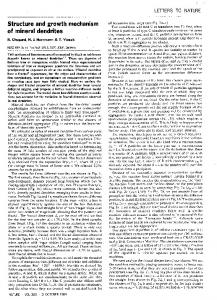
Figure 2.1: A schematic drawing of a generic neuron. Note that the main parts of the neuron in this picture are the axon and the cell body (soma). Picture adapted from http://www.epilepsyfoundation.org/about/science/images/Neuron.jpg see that the dendrites are in fact a very large part of the neuron. The Purkinje cell that is shown in this picture is the type of neuron with the most extensive dendritic tree. Here we are making special note of the vast spatial extension of the dendritic tree as this is the central concept of this thesis.

Figure 2.2: A drawing of a Purkinje cell from a cat’s cerebellum cortex done by Santiago Ramón y Cajal. The axon is the segment denoted a. The soma is the body where the axon ends. The rest of the neuron consist of dendrites. Before venturing further into the modelling of dendrites we will present a short history of neuroscience. As we discuss the breakthroughs and the people that made them, we will simultaneously describe the possible function and role of neurons. Neuronal morphology was first explored in the work of Santiago 6

C HAPTER 2: B ACKGROUND Ramón y Cajal and Camillo Golgi in the late 19th century. The first detailed description of dendrites was made by Golgi. He developed a revolutionary technique of silver staining [11]. Even if Golgi could identify the dendritic structure he considered the dendrites to simply be a support organ for the neuron, that held and distributed nutrients. Cajal looked at brain slices from cats, birds and other animals through a microscope and produced detailed drawings of neurons as can be seen in figures 2.2 and 2.3. Cajal was the first to come to the conclusion that a neuron is an independent unit that works together with other units to create a network. In figure 2.3 we see a part of the optic tectum of a sparrow. We see that each neuron is individually drawn in great detail both in the upper pyramidal cell layer and in the lower granule cell layer. By looking at this and other drawings done by Cajal it is easy to draw the conclusion that dendritic structure accounts for the majority of the surface area of the neuron. We will later elaborate on dendritic structure and what effect it has for the function of a neuron. Cajal also proposed the idea that the neuron receives information in the dendrites and that this information then flows through the soma where it is directed into the axon. Cajal called this “the rule of dynamic polarisation” [12] and he drew these conclusions purely by looking at the spatial distribution of neurons. In 1952 a big breakthrough in neuroscience was made as Hodgkin and Huxley released their paper “A quantitative description of membrane current and its application to conduction and excitation in nerve” [14]. Across the neuronal cell membrane there is a potential jump that is maintained by different ion concentrations on different sides of the membrane. The resting potential of a typical neuron is -65 mV. If the neuronal membrane is sufficiently depolarised active ion pumps in the membrane are activated and the membrane potential is then reversed temporarily. This reversal of membrane potential is known as an action potential (AP). The AP will travel across the membrane and induce a travelling depolarisation. This depolarisation can cause activation of ion pumps on other parts of the membrane. Especially along the axon the density of ion pumps is high and the action potential will travel down the axon. It was previously known that neurons fire APs [15], but Hodgkin and Huxley managed to accurately record the AP in a giant squid axon and even create a mathematical model of the membrane. The model included active Sodium, Potassium and leak currents that were able to mimic the AP in the giant squid axon. See ap7


Figure 2.3: Ramón y Cajal’s drawing of the optical tectum of a sparrow. We can easily identify granule cells at the bottom of the picture and above them we see a variety of pyramidal cells [13]. pendix 8.2 for details on the Hodgkin-Huxley dynamics. For this work Alan Lloyd Hodgkin and Andrew Huxley received the 1963 Nobel Prize in Physiology or Medicine and this is still today regarded as the basic model of how the neuronal membrane works. The three currents identified by Hodgkin and Huxley are not sufficient to explain all kinds of AP generation and dynamics seen in other types of neurons, but the model is easily generalised. As new ion channels and dynamics have been identified experimentally, modellers have been able to introduce new terms that are all of the same general form as the original Hodgkin-Huxley currents [16–18]. The original Hodgkin-Huxley model is four dimensional, as V and the three gating variables are governed by differential equations. Adding further currents can give a more realistic model but it will also add to the complexity of the model. To perform mathematical analysis of neurons there are also models that aim to reduce the number of dimensions while still maintaining biological significance. The oldest and also most used of these models is the integrate-andfire (IF) model presented by Lapicque in 1907 [19, 20]. The original IF model has

8

C HAPTER 2: B ACKGROUND the dynamics

V (t) − V0 dV (t) + I, =− dt rm

(2.1.1)

where V (t) is the neuron potential, V0 is the resting potential, rm the membrane resistivity and I is any injected current. In the model we also have a threshold value, h, and when V (t) ≥ h the membrane potential is restored

so that V (t) = V0 . The reaching of the threshold and resetting is mimicking

the firing of an AP in the neuron. The actual shape of the AP is not included but we have here a one dimensional and linear description of excitable tissue that allows mathematical analysis of the model. These low dimensional models are, however, not meaningless from a biological perspective, as IF models and developments of these are, for example, commonly used to model auditory neurons in the cochlea [21, 22]. There are also non-linear models of lower dimensionality than the Hodkin-Huxley model that are able to give the AP in more detail. Two specific examples that we will present in chapter 4 are the FitzHugh-Nagumo model [23, 24] and Morris-Lecar model [25, 26]. Both of these are planar (two-dimensional) models of excitable tissue that are widely used in theoretical neuroscience.

Figure 2.4: The transmission of neurotransmitter from the axon terminal to a postsynaptic membrane. Picture modified from Julien [27]. We have mentioned that the neurons are individual units that work together with other units. We would now like to present the means available for neurons to communicate with each other. As we described above, the AP will travel down the axon and finally end up at the axon terminal, see figure 2.1. At the axon terminal we find a chemical synapse. Here the pre-synaptic membrane, in our case the axon, and the post-synaptic membrane are separated by approximately 20 nm, a space called the synaptic cleft. In the pre-synaptic membrane 9

C HAPTER 2: B ACKGROUND there are synaptic vesicles containing neurotransmitters. When the AP arrives at the terminal, neurotransmitter is released and diffuses across the synaptic cleft to the post-synaptic membrane. Neurotransmitter is then absorbed by postsynaptic receptors and a post-synaptic potential (PSP) is induced in the postsynaptic neuron. This is a complex process and the PSP can either be caused directly by the neurotransmitter release or via a biochemical chain. The PSP can either be inhibitory or excitatory depending on the neurotransmitter that is involved in the synaptic transmission. There are numerous neurotransmitters but here we would like to mention the gamma-amino-butyric acid (GABA) which is inhibitory and the glutamate which is excitatory [28, 29]. In figure 2.4 we see a drawing of an active chemical synapse. In this case the axon terminal is connected to the dendritic membrane, which is the most common case, but chemical synapses can be formed between an axon and any of the fundamental parts of a neuron. The chemical synapses are the dominant means of communication in the mammalian brain but it is not the only channel. There is also gap junction coupling between neurons. The gap junction is a cluster of connexin proteins that allows ions to flow from one neuron to another. The chemical synapses we have seen so far are only active when the pre-synaptic neuron fires an AP but the gap junction is always active and therefore voltage fluctuations that are too weak to cause an AP can be communicated. Gap junctions are also normally bidirectional which means that the strictness of pre/post-synaptic neurons we saw for chemical synapses does not exist. Another speciality of gap junctions is that they do not exclusively exist at axons. Gap junctions can exist between any of the three fundamental parts of the neuron [30–32]. We will further consider gap-junctions and their effects in chapter 5. As the work in this thesis is focused on dendrites, we would also like to point out that neurotransmitter release is not only possible at the site of chemical synapses. In for example Purkinje cells and in the olfactory bulb magnocellular neurons (MCNs), the peptides vasopressin and oxytocin are released from their somato-dendritic compartment [33, 34]. These neurotransmitters then diffuse and affect other neurons in the proximity. As we have already stated, the brain contains approximately 1012 neurons and for this reason there is use for coarse grained models of brain tissue. This type of modelling is often referred to as neural field theory and has been developed 10

C HAPTER 2: B ACKGROUND by H. Wilson, J. Cowan, S. Amari, P. Nunez and H. Haken, for a review see [35]. In particular it is useful for the theoretical study of EEG rhythms and working memory [36, 37]. However, we will not treat this level of description here.

2.2 Biology and Morphology of Dendrites 2.2.1 The Dendritic Tree As we have seen in figures 2.2 and 2.3 the dendritic structure of neurons can be up to 90 % of the total surface area of a neuron. With this fact it is natural to start looking at the morphology of the dendritic structure. The diversity of shape in different dendritic trees is striking. We have as extremes the selective arborization of an olfactory sensory cell and the space filling structure of a cerebellar Purkinje cell. In between these we have a variety of sampling arborizations such as the pyramidal cell in the cerebral cortex [38], see figure 2.5 for some dendritic morphologies. During the early development of the brain the dendrites grow out from the cell body to create the dendritic structure. The development of the dendrites is partly dependent on genetic factors and cell lineage but is also activity guided. If the growing dendrites recieve synaptic input and interact with glial cells, this encourages further development. The devlopment and guidance of this growth is a complex biochemical process that we will not go more into here. For further details see [39]. This process has also been thoroughly studied in a theoretical context to recreate realistic dendritic arborisations, see for example the work of Graham and van Ooyen [40, 41]. As we have seen, dendrites can often be branched in a very complicated manner but we have no closed loops in the dendritic structure, see figure 2.5. This is known as a tree structure, which we will now proceed to give some background on. The tree is a structure that is used in fields other than neuroscience, such as computer science [44] and lung mechanics [45]. In the work by van Pelt and Schierwagen [43] the following parameters, that also can be seen in figure 2.6, are used to characterise trees: Order. This is how many levels the tree consists of, counted from the soma. The branches that connect directly to the soma have order 0. The daughters of these branches then have order 1 and so the order increases all the way to the 11


Figure 2.5: Examples of dendritic trees. (a) Cat spinal motoneuron. (b) Locust mesothoracic ganglion spiking interneuron. (c) Rat neocortical layer 5 pyramidal neuron. (d) Cat retinal ganglion neuron. (e) Salamander retinal amacrine neuron. (f) Human cerebellar Purkinje neuron. (g) Rat thalamic relay neuron. (h) Mouse olfactory granule neuron. (i) Rat striatal spiny projection neuron. (j) Human nucleus of Burdach neuron. (k) Fish Purkinje neuron. Modified from [42]. terminal segments. Degree. This is the number of terminal tips that belongs to a subtree. If the segment we are looking at is the root of the tree, then the degree is simply the total number of terminal tips in the tree. Asymmetry index. This is a parameter that expresses the probability that any segment should branch asymmetrically at any of the n − 1 branch points in tree with degree n. This can be calculated with the summation A=

1 A p (r i , s i ), n−1∑

(2.2.1)

where (ri , si ) is the degree of each subtree at branching point i. The partition asymmetry, A p , is defined as Ap =

|r − s | r+s−2

for

r+s >2

and

A p (1, 1) = 0.

(2.2.2)

That means that a perfectly balanced tree has A = 0 while the most asymmetric 12


Figure 2.6: Some terminology for a arbitrary tree structure (A) is shown as well as the degree (B) of the sub-trees and finally we have the order (C). This image is adapted from [43]. tree has A = 1. These values are common for all types of trees but we need a bit more information to describe a dendritic tree. The values above only describe the connectivity of the nodes in the tree and we are equally interested in the morphology of the edges since those represent the dendritic segments. For each segment we need to know the length and the diameter. The diameter is often a function of the distance from the soma, particularly for tapered dendrites [46]. One important difference between dendritic trees and the ones used in many other cases is that a biological dendritic tree has more degrees of freedom. If we want to analyse the effects of morphology on the electrical properties of a neuron we can not ignore the fact that a neuron is a three dimensional structure. A theoretical framework of how to classify three-dimensional trees is presented by da Costa et al., [47]. Here, three families of measures that are needed to classify and describe a three-dimensional tree structure are presented: Differential Geometry. This family includes measures such as segment length, curvature and orientation. Symmetry axes. These are the measures that describe how the tree is built stored. These measures are, for example, hierarchical representation and the number of branches in the tree. Measures such as order and degree fit into this family. Complexity. These are measures that describe the neuron as a whole. Examples are fractal dimension and extension of the dendritic tree. The appealing aspect about the work by da Costa et al. is that many other papers that discuss morphological properties of dendrites can be said to focus on measures that can quite easily be identified as part of this framework. In a 13

C HAPTER 2: B ACKGROUND follow up paper by Barbosa et al. [48] the complexity issue is further explored with the help of Minkowski functionals that have been gathered in a framework called Integral-Geometry Morphological Image analysis. Ascoli [49] is discussing some differential geometry measures in his paper for 1999. Ascoli suggests that to fully describe a three-dimensional branch point we need the following three values: Amplitude. A number that gives the angle between the two daughter segments after the branching. Elevation. The branching’s tilt with respect to the parent segment. Azimuth. The torque of the branching with respect to the parent segment. The more detailed differential geometry of the individual segments is explored in the work of Streekstra and van Pelt where they use Gaussian kernels to describe the centre line position and diameter of dendritic segments [50]. As dendrites are the main site for synaptic input it is natural that we would like to have as much area as possible where contacts can be formed. On the other hand, a large dendritic volume and a long dendritic cable are not energy efficient, and will slow down certain types of signalling that depend on diffusion. This seems to favour a compact and highly branched dendritic structure. Indeed, by optimising dendritic volume for a given total wiring length, the dendritic structure of fly neurons has been successfully reconstructed [51, 52]. Not all dendritic arborisations strictly follow this optimisation principle. Pyramidal cells that we can see in figure 2.3 receive inputs from multiple layers in cortex, and the dendritic tree is then shaped to accommodate this. The role of dendritic structure stretches beyond simply being a place where synaptic connections are made. The dendritic morphology influences the response in a way that causal relationship between dendritic structure and firing properties in neocortical neurons can be concluded. In the case of passive dendrites, different morphologies mainly affect the firing frequency of neurons. If active currents in the dendrites are considered, we also see more qualitative differences, such as the firing patterns varying between bursting and regular patterns [53, 54]. In a similar manner the morphology affects the back-propagation of action potentials [55].

14


2.2.2 Dendritic Spines

Figure 2.7: Three dimensional imaging of a spiny dendrite [56]. Many axo-dendritic synapses are situated on dendritic spines [29]. Especially excitatory synapses are often placed on spines. Dendritic spines are small protrusion on the dendritic cable on the 1 µm scale. The spines can come in many shapes and variations. In general all dendrites can be classified as spiny, sparsely spiny or smooth but even neurons with smooth dendrites usually have a few spines. There are also a number of different shapes associated with the spines [38]. In figure 2.7 we see a piece of spiny dendrite with mainly what are known as simple spines. We can divide spines into simple and branched spines where the simple spines consist of a spine neck connected to a more bulbous spine head. As expected, the branched spines are simply two or more spine heads connected to a common spine neck. In figure 2.7 we further see that even the simple spines can have considerable variations in shape. The spines serve to create biochemical microenvironments that receive input from other neurons and compartmentalise the postsynaptic response from the dendritic cable; in that way the spine can serve to boost the synaptic input [57, 58]. As so much of the synaptic input is located at the spines, they are critical for dendritic integration [59]. As we have seen, the shape of the spines can vary, and with that the electrical properties such as membrane resistance and conductance are also different between spines. It has been shown that these variations develop 15

C HAPTER 2: B ACKGROUND over time and are dependent on the activation of the synapses [60, 61]. Spines therefore play an important role in neural plasticity.

2.2.3 Active Currents in Dendrites When we described the function of the neuron in section 2.1, the neuron had active, voltage gated current of the type that was first described by Hodgkin and Huxley. These currents are most common in the soma and along the axon, but voltage dependent currents are also present in the dendrites. Theories of this type were originally proposed by de No [62] and also by Wilfrid Rall [63, 64]. Rall is closely connected with the passive cable theory but he was actually one of the first to examine the non-linearities in dendrites. Despite these early explorations, it was not until the early 1990’s that direct demonstrations of voltage gated ion channels in dendritic structure were made. Through dual recordings of the soma and dendrites of pyramidal cells by Stuart et al., it was shown that action potentials initiated in the soma are capable of invading the dendritic tree [65, 66]. These back propagating action potentials (BPAPs) exist to a certain degree in a passive structure due to diffusion, but Stuart et al. make clear that the measured BPAP could not be explained by this alone. Further recordings also verified that active mechanisms amplify synaptic input [67]. In the past 15 years since these observations, numerous voltage gated channels have been identified. We have the Sodium and Potassium channels that are used in the original Hodgkin-Huxley model. In the dendrites, the Sodium channels can initiate non-linear effects that we know as dendritic spikes [68– 70]. Calcium and Chloride channels have also been identified, as well as other non-specific channels [71, 72]. Among the non-specific channels, the hyperpolarising current, h-current, is of special interest, as it has been shown to be abundant in the distal parts of CA1 pyramidal neurons [73, 74]. In a recent review by Johnston and Narayanan [75] the following eight points are presented to summarise the roles and observations in the field of active dendrites. 1. Na+ -dependent APs that are initiated in the soma or the axon backpropagate through the dendrites supported by voltage-gated channels. 2. Na+ -dependent spikes can be initiated in the dendrites. These dendritic 16

C HAPTER 2: B ACKGROUND spikes can be of a local type but can also start off a more global phenomena in the dendritic structure. 3. Ca2+ channels are opened by both BPAPs and local dendritic spikes. This channel activation will produce a rise in intracellular Calcium. 4. In distal dendrites Ca2+ -dependent spikes can be sustained. 5. A rise in intracellular Calcium can also be obtained by the opening of Ca2+ channels due to synaptic input. 6. In some neurons K+ channels regulate the BPAP and play a role in the initiations of dendritic spikes. 7. Dendritic h-channels are important in the integration of temporal patterns and can also mediate neuronal oscillations. 8. The distribution of voltage-gated channels (together with dendritic morphology) influences the type of output of a neuron for a given input [53, 54, 76]. As we will see in section 2.4 active properties also have great importance for the plasticity of the neuron. There is, however, much more to be done when it comes to the mechanisms and the role of active currents in dendrites. This is true from an experimental as well as from a theoretical point of view. In the following section we will consider some of the landmarks in dendritic modelling and we will, among other things, touch on the theoretical treatment of voltage-gated channels in dendrites.

2.3 Modeling of Dendrites 2.3.1 The Passive Cable and Rall’s Model Neuron To begin the journey through dendritic modelling we will start with the theory of passive dendrites. The story of cable theory and dendrites is in many ways the story of one man, Wilfrid Rall. After Hodgkin and Huxley’s model of the squid giant axon, the field of making electrophysiological recordings from neural tissue opened up. Among the first successes was the group of Eccles that 17

C HAPTER 2: B ACKGROUND made recordings from motoneurons to determine membrane properties. Eccles included dendritic structure in a model, but the size of the structure was greatly underestimated. In addition to this, Eccles calculations suggested that synapses placed on the dendrites are at such great electronic distances from the soma, that these synapses would not affect the voltage in the soma at all. In 1957, Rall published a letter in Science that highlighted that the time-course of the voltage in the motoneuron was closer to that of dendrites with no soma, than to the time-course of a soma without dendrites [77]. In 1959 Rall presented the theory that he became most famous for, namely the cable theory for neuronal dendrites. Cable theory had been applied to axons even before Hodgkin and Huxley’s non-linear theory in order to examine the passive properties of the axon [78, 79]. The electrical properties of a passive dendritic segment can be described by the cable equation ∂V ( x, t) rm ∂2 V ( x, t) rm cm = − V ( x, t) + rm Iinj ( x, t), ∂t ri ∂x2

x ∈ R,

t > 0. (2.3.1)

Here V ( x, t) is the transmembrane potential, rm is the membrane resistance of unit length times unit length (Ωcm) and cm is the membrane capacitance per unit length (F/cm). Iinj ( x, t) is an applied current density. We will also use a and ri , that denote dendrite radius and axial resistance respectively, later. For derivation of the cable equation see [80]. 1500

1000

500

0

−500

−1000

−1500 −1500

−1000

−500

0

500

1000

1500

−2000 2000 2000 0

Figure 2.8: Typical morphology of a motoneuron like those Rall [78] as well as Coombs, Eccles and Fatt [81] made recordings from. The morphology data was taken from http://krasnow.gmu.edu/L-Neuron/L-Neuron/database/index.html#Moto 18

C HAPTER 2: B ACKGROUND If we consider an infinite cable, the solution of (2.3.1) can be written as V ( x, t) =

Z t 0

ds

Z ∞

−∞

dyG ( x − y, t − s) Iinj (y, s) +

Now, let τ¯ = rm cm , λ =

√

2arm /ri and D =

¯ λ2 /τ.

Z ∞

−∞

dyG ( x − y, t)V (y, 0).

(2.3.2)

The Green’s function for the

infinite uniform cable may be written G ( x, t) = √

1 4πDt

e−t/τ¯ e− x

2 /(4Dt )

,

−∞ < x < ∞, t > 0.

(2.3.3)

In the original paper by Rall [78], he considers the steady state solution for the cable equation, ∂V/∂t = 0. In table 2.1 we see the steady state solution for the cable equation in the case that we have current injection at x = 0 in a dendritic cable. We consider a semi-infinite cable and two cases of a finite cable for which 0 ≤ x ≤ l. The two cases of finite cable we consider are a cable with a closed end, V (l ) = 0, and open end, ∂V/∂x | x=l = 0.

Semi-infinite cable Closed end at x = l V (0 )

Iinj ri λ V (0)e− x/λ

Iinj ri λ coth(l/λ) cosh(l − x )/λ V (0) cosh(l/λ)

Open end at x = l Iinj ri λ tanh(l/λ) sinh (l − x )/λ

V (x) V (0) sinh(l/λ) Table 2.1: The steady state solutions of the cable equation in the case of current injection at x = 0 for three cases of dendritic cable. We show the solution at the place of current injection, V (0), and as a function of x. Applying the cable equation to dendrites was without doubt very important, but Rall also took other measures to handle dendritic geometry. As the axon is usually less branched, at least proximal to the soma, the cable equation was a natural application to this part of the neuron. In chapter 7 we will further discuss the use of the cable equation in connection with axons. The dendrites, on the other hand, are usually constructed by many short branches, so to apply the cable equation to each of these with the correct boundary conditions would be a very complicated task. Rall was able to derive the 3/2 power law that allowed for the construction of an equivalent cylinder. To construct an equivalent cable for a branching point in the tree, the radii of the branches, ai , must obey [82]. See right part of figure 2.9 for an example of a branching a3/2 = ∑i 6= j a3/2 i j point that can be collapsed to an equivalent cylinder. The resulting equivalent cables radius, a, is determined by a = A/2πL, where A is the total surface area of the tree and L is the total length of all the branches. The length of the equivalent cable is chosen so that the electrotonic length of the cable is the same as 19


a

2

a

1

a

3

a

Figure 2.9: Left: The compartmentalisation of the passive dendritic cable. In this figure Ra is the axial resistance of the cable, Rm is the membrane resistance, Cm is the membrane capacitance and a is the cable radius. Right: A schematic picture of how to create an equivalent cable of a branching node. The requirement for this is that 3/2 = a3/2 a3/2 2 + a3 , where ai is the radii of each branch. The radius of the equivalent 1

cable is a = A/2πL, where A is the total surface area of the tree and L is the total length of all the branches, i.e. L = ∑i li . the average electrotonic length of the whole tree. The electrotonic length of a p cable with length lk is lk /λk , where λk = (rm ak )/(4ri ) [83]. The resistances rm

and ri are the membrane resistance and the cables axial resistance respectively,

see figure 2.9. By the equivalent cylinder approach and the cable equation, Rall was able to make excellent predictions of the parameters in the motoneuron membrane and thus become the first to effectively include a spatially extended dendritic structure in a neuron model. A more general representation of these equivalence transforms is presented by Lindsay et al. [84]. This paper explains how an uniform Y-junction can be mapped into an unbranched structure whose total electronic length is the same as the total electronic length of the branched structure. Any dendritic tree can then be seen as a system of parallel and serial Y-junctions. In [85], Reeke et al. apply this scheme to large branched structures. In 1964 Rall produced yet another paper that came to be a landmark in the modelling of dendrites. The limitations of the equivalent cylinder model motivated the development of the compatmental model [63]. The core idea in compartmental modelling is that a part of the dendritic cable is described by an electric circuit. In the case of Rall’s original idea, this is a circuit that describes the passive properties of the membrane. In figure 2.9 we see how the dendritic cable is approximated by a chain of these circuits coupled by resistances. This is a nat20

C HAPTER 2: B ACKGROUND ural discretisation of the dendrites, and compartmental modelling has been the dominating paradigm in the modelling of neural structure in general and especially for dendrites. For example, widely used programs such as NEURON and G ENESIS implement compartmental modelling [86, 87].

2.3.2 Morphoelectrotonic Transform In the previous section we spent some time considering dendritic morphology and what effect this has on the response of neurons. We also introduced cable theory for passive dendritic structures. Now we will discuss a measure that connects the two fields. The morphoelectrotonic transform (MET) is used to visualise voltage attenuation or delay of the voltage waveform in the neuronal structure. MET was introduced by Zador et al. in 1995 [88]. Let’s look back at equation (2.3.2). If we assume that V ( x, 0) = 0 and we inject a current Ii (t) = I A ( xi , t) at a point xi in the dendritic tree. The voltage Vj (t) = V ( x j , t) at any other point x j in response to Ii (t) is Vj (t) =

Z ∞

−∞

Ii (s)Gij (t − s)ds = Ii (t) ∗ Gij (t),

(2.3.4)

where ∗ indicates temporal convolution. Gij (t) is the Green’s function between

the points xi and x j , i.e. Gij (t) = G ( x j − xi , t). By taking the Fourier transform, yˆ ( f ) =

Z ∞

−∞

y(t)e−i f t dt,

(2.3.5)

where the notation yˆ( f ) means the Fourier transform of y(t), of equation (2.3.4) we get Vˆ j ( f ) = Iî ( f )Gˆ ij ( f ).

(2.3.6)

The voltage attenuation between two points is Aij ( f ) =

Vî ( f ) Gˆ ( f ) = ii . Vˆ j ( f ) Gˆ ij ( f )

(2.3.7)

This expression is not additive, and that is a property that is desirable for us as we want to visualise the attenuation. We could visualise the non-additive measure, but in that case it is not so easy to differentiate between electronically compact and distant regions. See the difference between the classic electrotonic diagram and the attenuation diagram in figure 2.11. By taking the logarithm we get Lij = log(| Aij ( f )|). 21

(2.3.8)

C HAPTER 2: B ACKGROUND The logarithmic attenuation is then used to draw an attenogram. This is done by taking the physical morphology of a neuron and rescaling it so that one unit length represents an e-fold attenuation. Note that only the length of each segment is re-scaled, the diameter and orientation are preserved. See figure 2.10 for an example of this.

Figure 2.10: An example of an attenogram. Notice how the attenuation is much higher in the branches that do not have an injected current. This image is reproduced from [88]. Another variant of morphoelectrotonic transform is the delay in the voltage waveform [82]. The delay is defined as the difference between the centroids of the voltage response at two separated points xi and x j [82, 89]. The centroid of a voltage response at xi is defined as R∞

ti = R0∞ 0

tv( x, t)dt v( x, t)dt

.

(2.3.9)

The delay is then calculated as

Pij = t j − ti .

(2.3.10)

This is then used to draw a delayogram much in the same way as the attenogram. In a delayogram one unit length represents a fixed delay time. Delayograms and attenograms are useful for visualising how different input frequencies behave in an branched structure. 22


Figure 2.11: An example of an attenograms and delayograms. See the text for details about the different transforms. This image is reproduced from [88].

23

C HAPTER 2: B ACKGROUND In figure 2.11 we see some morphoelectrotonic transforms of a pyramidal cell from layer 5 of cat visual cortex. Beginning from top left we see: a. The three-dimensional anatomical reconstruction of the neuron. b. In the middle of the top row we have the classical electrotonic transformation where the length of each process is replaced by its electrotonic length, L = l/λ, that is dependent on fiber geometry. c. Top right shows a centrifugal attenogram where the current is injected into the soma. Note that, as opposed to the classical electrotonic transformation, here an electronically distal branch gets shorter than in the real geometry. d. Bottom left is an attenogram where instead current is injected in each of the dendritic terminals; this is called a centripetal attenogram. Note that the scale is different than in c. The small insert at the side shows the centrifugal attenogram drawn in the same scale. e. Finally we have the somatic, centripetal delayogram with its centrifugal counterpart. Figure 2.11 is adapted from [88].

2.3.3 Modelling Active Currents When we described the dendritic membrane containing voltage-gated channels we noted that the non-linearities were not directly demonstrated until the early 1990’s by Stuart et al. [65, 66]. However the transient nature of dendritic processing and synaptic input was known earlier, and in two papers in 1973 and 1975 Rall and Rinzel gave a mathematical formulation of these transient currents [90, 91]. These transients are detected as an overshoot or undershoot as current is injected, see figure 2.12 for an example. Rall and Rinzel applied their transients theory to an idealised dendritic tree, but Butz and Cowan derived a scheme to use transients in a arbitrary geometry [92]. Further development was made in this area when Koch and Poggio in the 1980’s showed that the formulations used earlier to describe transients can be obtained by linearising general non-linear currents [93, 94]. We will not go into more detail of these formulations of transients and linearised currents here, as in chapter 3 we will use these to fit experimental data. Here we will thoroughly discuss the derivation of linearised currents and what effects they may have for dendritic process24

C HAPTER 2: B ACKGROUND ing. When we come to the history of modelling non-linearities in the dendrites

Figure 2.12: To the left we see a voltage trace with a transient overshoot as current is injected. The circuit to the right describes the membrane dynamics that give the transient. we again have to credit Wilfrid Rall for his important contributions. In 1985 Miller, Rall and Rinzel published work discussing the active amplification of synaptic input in the dendritic spines [57]. Baer and Rinzel later developed the amplification model for synaptic input in the spines to incorporate a spatial dimension [95]. The resulting Baer-Rinzel model makes use of a continuous description of active currents. The dendritic spines are described by a continuous spine density along the dendrites. The most significant contribution to the modelling of active dendrites from Rall is, however, the compartmental model. It is straight-forward to supplement the passive circuits seen in figure 2.9 with pathways that contribute with non-linearities. This allows for detailed reconstruction of the dendritic tree, with voltage-gated currents in the membrane. With this framework, some impressive results have been produced that are able to give an account of non-linear activities in dendritic structures. An example of this is Jarsky et al. that investigates the activity in a reconstructed CA1 hippocampal pyramidal cell [96]. Models of the BPAP also makes it possible to examine communication within a single neuron. As a firing event can propagate and be detected through the entire neuron, not just the soma and axon, this can be important for plasticity and feed-back [97, 98].

25


2.3.4 Coincidence Detection

Figure 2.13: Schematic picture describing the morphology of a bipolar neuron. The next success story of dendritic modelling we would like to get across, is that of the importance of dendrites in coincidence detection. Mammals and birds use sound to identify the location of both prey and predators. By using intra-aural time differences, the sources of sounds can be located. We will consider a bipolar neuron, i.e. a neuron that has a dendritic arborization that is extended in two directions that are opposite to each other [29], see figure 2.13 for a schematic picture. The input from left and right ear will come onto the different parts of the dendritic arborization. The idea of coincidence detection in the auditory system was first presented by Jeffress in 1948 [99]. A paper by Agmon-Snir et al. published in 1995 clearly demonstrated the importance of the dendrites for coincidence detection [100]. This is demonstrated by considering two biophysical mechanisms. The first mechanism is the spatial segregation of inputs. This allows for non-linear integration of the input from the left and the right ear. The other mechanism is that the opposing dendritic tuft acts as a current sink for the input. In audition, coincidence detection is easy to interpret from the type of input. If the sound reaches both ears at the same time, then we have coincidence. Coincidence detection has also been shown to play an important role in the visual system. In vivo experiments on macaque monkeys performing a motion-detection task demonstrated that coincidence detection is present in the middle temporal area of the visual system [101]. By considering the morphology of a pyramidal cell, Agmon-Snir et al. also suggested that 26

C HAPTER 2: B ACKGROUND coincidence detection is a feature in higher brain areas, i.e. areas that are further from receiving direct sensory input. Pyramidal cells have a more complex branching pattern than bipolar neurons where the dendrites can be divided in a basal tree below the soma and the apical tuft above it, see figure 2.3. Coincidence detection in pyramidal cells is later explored by Schaefer et al. who conclude that dendritic morphology is a critical factor for coincidence detection [102]. Schaefer et al. do not offer any explanations as to what kind of coincidences are detected by pyramidal cells, or what role they play. Other studies, however, suggest that coincidence detection in hippocampal granule cells is involved in memory recall [103]. In conclusion, we can say that a problem and model that were presented by Jeffress in 1948 was further developed and thoroughly explained in 1995 by simply considering the dendritic structure of a neuron. This is an excellent example of the importance or dendritic processing and how seemingly complicated mechanisms can easily be explained by including spatial structure. The ground breaking work of Agmon-Snir et al. has also started a number of studies on the importance of coincidence detection in cortex and hippocampus, but in these areas there is still much work to be done.

2.4 Plasticity and Learning 2.4.1 Machine learning We will here introduce some of the theory and notation used in machine learning. As the field of machine learning in general and artificial neural networks (ANNs) especially, are highly influenced by neuroscience, this is a good way to introduce learning concepts. First of all, we will present the idea of a classification task and a learning object. The object we teach, what we will call the learning object, can generally be a lot of things in practise, but in every case, there is a computer program that is adapting itself over time. One of the most successful self learning objects is TD-Gammon [104], which is a program that plays backgammon. In the beginning the program only knew the basic rules of the game, and it learnt by playing against itself. After 1,500,000 training games, the program was ready to take on the backgammon grand master Bill Robertie. The result was that man won over machine; Robertie won 21 out of 40 games. We can easily think of a general task that we want to teach an artificial system, 27

C HAPTER 2: B ACKGROUND i.e. playing backgammon, reading a text, or driving a car. When we break it down, the task is to make decisions, given certain information. We will call this task pattern classification. For TD-Gammon the input pattern is the layout of the playing field and the roll of the dice; based on this, the program has to make a decision about what is the most effective next move. The term “pattern classification” makes good sense in the case of text recognition, as each letter that is read is matched against a finite number of possible classes, i.e. the alphabet, and then the most appropriate letter is chosen [105]. The classification method is dependent on the type of the learning object. We will now present the first learning object that we focus on here, namely the perceptron.

Figure 2.14: Schematic drawing of a perceptron. The perceptron is the simplest form of an artificial neural network (ANN). It is actually a one-layer, feed-forward ANN; see figure 2.14 for a schematic picture of the perceptron. The concept of ANNs has been around since McCulloch and Pitts introduced it in the 1940’s [106]. In their work McCulloch and Pitts treat a neuron as a simple binary operator that produces 1 if the input to the neuron is above a certain threshold, µ. This can formalised by N

y = Θ ( ∑ w j x j − µ ),

(2.4.1)

j =1

where Θ is Heaviside step function, x j are the inputs to the neuron and w j is a weight that is associated with the jth input. The output, y, can then be used as input to other neurons. The learning in ANNs is generally conducted by updating the input weights according to the rule w j ← w j + ∆w j ,

(2.4.2)

∆w j = λ(t − y) x j .

(2.4.3)

where

28

C HAPTER 2: B ACKGROUND In the update, t is the target value for this input and λ is the learning rate. The details of how this update is done are dependent on which learning paradigm and type of learning rule that are chosen [107]. ANNs were inspired by the observation that the human brain is built by seemingly simple units and through the intricate network structure is able to perform a wide range of tasks. In the 1940’s research into plasticity started to take off with the work of Donald Hebb in the fore-front [108]. We will come back to Hebb’s theories later. ANNs also have roles in neuroscience. They generally do not attempt to simulate a biological network of neurons but are rather used as a classifier to test the effect of experiments. This is a task they have proved to handle very well. In this context ANNs have been proposed as a classifier of cognitive impairment and therapeutic effectiveness in Alzheimer’s transgenic mice [109]. ANNs take input data and make a decision about which class the pattern belongs to. The input to an ANN is, as can be seen in (2.4.1), a vector of N input values that we call x. Each of these inputs is weighted by an element in a weight vector, w. The equation w · x = 0 then describes a hyperplane that divides N dimensional space into two parts. With training we want to adjust the weights so that all patterns on each side of the hyperplane are of the same class. The perceptron is limited in the sense that it is a linear classifier. If the patterns we wish to classify are not separable by a hyperplane, we can introduce a multi-layered ANN where the output from one layer becomes the input to the next layer. In a multi-layered structure we also have the possibility to introduce feed-back loops. By this architecture, arbitrary regions in our N dimensional space can be separated from each other [105]. We will in chapter 6 briefly revisit the perceptron and generalise it to include spatial extension. So now we have given an example of a learning object, the perceptron, and how it classifies patterns. We also saw the learning rule for the perceptron, though as yet we have not really considered how we can teach a system to solve a given classification task. There are two main learning paradigms, supervised and unsupervised learning. Supervised learning involves an external teacher that tells the system if any adjustments are necessary. The perceptron update rule (2.4.3) is an example of a supervised learning rule as the current output is compared to a desired output. An example of an unsupervised learning rule is Bayesian learning [105]. In Bayesian learning there is a space of hypothesis, H, and a set of training data, D. An hypothesis, h, is chosen from H and then the 29

C HAPTER 2: B ACKGROUND most probable hypothesis is determined by taking arg max P(h| D ). hǫH

(2.4.4)

This can be evaluated using Bayes theorem P (h | D ) =

P ( D | h ) P (h ) . P( D )

(2.4.5)

We will not elaborate on different learning rules. For further information on neural networks and machine learning we would like to refer the reader to the works of Jain et al. [107], Mitchell [105] and Bishop [110]. In chapter 6 we will further study a few learning rules that we feel have closer connection to biology and especially spatially extended dendrites.

2.4.2 Neural Plasticity One of the major challenges in neuroscience is to gain deeper understanding of how memory and learning work. Among the first and definitely most famous people to examine learning was Ivan P. Pavlov during the end of the 19th and beginning of the 20th century. In his famous experiments he conditioned dogs so they started salivating at the sound of a bell. This was because the dogs learnt that the sound of the bell was usually followed by food. Pavlov also presented quite elaborate ideas about how sleep influences learning and which brain areas might be involved [111]. Every day new memories are created and deleted in humans and animals. This must all be done with the greatest care because if essential memories or skills are deleted this would have severe implications for everyday life. These memories and skills are stored in both the network properties of different brain areas [112] as well as the intrinsic excitability of single neurons and their synapses. All these quantities are dynamic and all changes are collectively referred to as plasticity. The theory of Donald O. Hebb is best summed up by his own words; "when an axon of cell A is near enough to excite a cell B and repeatedly and persistently takes part in firing it, some growth process or metabolic change takes place in one or both cells such that A’s efficiency, as one of the cells firing B, is increased“ [108]. Although the theory of neural plasticity has been developed since Hebb, the idea of activity dependence is still a central concept in plasticity. Hebb’s activity driven plasticity has been experimentally verified by Bliss and Lømo [113] by high frequency stimulation of 30

C HAPTER 2: B ACKGROUND pre-synaptic neurons. The synapses between the pre and post-synaptic neuron are strengthened by applying this stimulation protocol. Plasticity is generally divided into intrinsic, structural, and synaptic plasticity. Intrinsic plasticity is concerned with how intrinsic properties of the neuron change. The conductance of dendrites and soma is one example of an intrinsic property that might change [114]. Structural plasticity is a collective term for the growth and retraction of dendrites and axons that allows new connections between neurons. Structural plasticity is mostly prominent during the development of the CNS and in the repair of injuries [115, 116]. Most of the structural plasticity takes place during the development of the brain [40, 41]. Synaptic plasticity occurs when an existing synapse gets weakened or strengthened. This change happens through either a change in the amount or release probability of neurotransmitter at the pre-synaptic side, or a change in the efficacy of neurotransmitter uptake at the post-synaptic side [117]. The effect of this is that the post-synaptic potential (PSP) in response to the arrival of an AP at the synapse will be either stronger or weaker than before. The strengthening of synapses is called potentiation and the weakening is called depression. The concept of synaptic plasticity is also widely used in machine learning applications as discussed in last section. As plasticity is such a central concept in neuroscience, several other discoveries and models are used to explain learning and changes in neurons. The dendrites are highly involved in this for a number of reasons. When it comes to synaptic plasticity the dendrites become an important factor as the majority of the synapses are located on the dendrites. As the dendrites represent such a big part of the neuronal surface it is also natural that structural plasticity is very dependent on the dendrites. In the mature brain, the growth and change in shape of dendritic spines also falls into the class of structural plasticity and is the most prominent example of this kind of plasticity [61]. Many things we have considered so far have been applied in the field of learning. It has, for example, been shown that the active currents of the dendrites play an important role. When Stuart et al. [65] first measured the BPAP this was soon picked up in the context of plasticity. The BPAP is seen as a feed-back mechanism from the soma that invades the dendritic structure. As the main part of the synapses is placed on the dendrites, this will indicate that the neuron has fired an AP. The feed-back mechanism is usually seen as a way to regulate the plasticity of the 31

C HAPTER 2: B ACKGROUND neuron [118–120]. We also have connections between coincidence detection and plasticity. Xu et al. [121] demonstrate this link in their paper published in 2006. In this case the plasticity is the tool that tunes coincidence detection. Note that in the link between BPAPs and plasticity it was the active currents that were the mechanism that facilitated certain types of plasticity, while in the link between coincidence detection and plasticity, it is the opposite. This is just a short introduction to neural plasticity in which we have presented the ideas of Hebb. Neuronal plasticity is one of the most well-studied areas in neuroscience and there are an enormous amount of models and literature. Plasticity also involves numerous disciplines, from physics and mathematically driven systems close to machine learning [105] to pure biological approaches on a molecular level [122]. In between there is naturally also work that combines biophysical structure with computational models such as compartmental modelling as we discussed in passive cable theory [123, 124]. We will not go further into the details of different learning rules or mechanisms for plasticity here. In chapter 6 we will present new learning rules as we apply them to a spatially extended neuron.

32

C HAPTER 3

Sum-Over-Trips and Quasi-Active Currents Tact is the ability to tell someone to go to hell, and have them look forward to the trip. - Anon In this chapter we will deal with the complexity of dendritic structure and identify a method to calculate the response function for a branched dendritic structure with quasi-active membrane. We will briefly review the path integral method for a passive branched structure and see how we can make use of databases containing morphological data to build realistic models of dendrites. We will also generalise the method to apply not only to passive dendritic membrane but to incorporate resonant properties. This gives us a method to calculate the response of any stimulus at any point on an arbitrary complex morphology without numerically integrating any partial differential equations (PDEs). We capture enough biophysical detail in our model to examine the possible effects of a spatially varying conductance associated with the mixed cation current Ih . Finally we match a model of the quasi-active membrane with experimental data from a rat CA1 hippocampal pyramidal cell.

33

C HAPTER 3: S UM -O VER -T RIPS

AND

Q UASI -A CTIVE C URRENTS

Figure 3.1: Two examples of trips that connect the point x on branch k with the point y on branch m.

3.1 The Path Integral 3.1.1 Sum-Over-Trips on a Branched Structure In section 2.3 we introduced the cable equation for a single passive dendritic segment. We also considered two approaches to applying the cable equation to a branched dendritic structure: the equivalent cable and compartmental modelling. In this chapter we will present an alternative approach to solve the voltage response on a passive branched dendritic structure. We will then generalise this approach so that we can consider dendritic membrane that is not just passive but can also have voltage dependent currents. We saw that the cable equation is solvable in closed form with the use of Green’s functions in the case of an infinite cable. To remind us let us write down the Green’s function for the infinite cable equation: G∞ ( x, t) = √

1 4πDt

e−t/τ¯ e− x

2 /(4Dt )

,

−∞ < x < ∞, t > 0.

(3.1.1)

What we want to do is find a formalism that allows us to calculate the response for a branched structure with the help of Green’s functions. This is possible 34


AND


by applying the Feynman formula for the path integral [125] to our system of branched dendritic segments. The method to calculate the Green’s function in different finite geometries is used in electrodynamics under the term “method of images” [126]. This approach for solving electrostatic and electrodynamical boundary value problems is also applicable to dendritic geometries. Instead of creating images of each dendritic segment we are considering, we travel through the tree via different paths. The path ends as we reach an end point or a node in the structure and a new path commences. The set of paths that connect two different points is what we will call a trip. For an infinite dendrite we only have one possible way to connect two points, as any path that passes through the points towards ±∞ will never be reflected and come back. There-

fore there is only one trip in an infinite system. If we instead consider the simple system of a finite cable we have an infinite number of trips. This is simply because at each end point of cable a new path begins and we travel back through one or both of the points we want to connect. The trips get longer and longer as we visit the end points of the cable more and more times but all the trips make a contribution to the problem we are trying to solve. To get the full answer we need to consider a sum over all the possible trips that we can make to connect the two points in question. Just as in electrodynamics we have to consider all the images. Therefore the name of this approach is "sum-over-trips". In the case of a finite system this sum is infinite but we will see that the contribution of the longer trips is low. The sum considered will have terms that are built up using (3.1.1) and x will be the length of the trip. Hence the terms will decay exponentially as the trips get longer. What has just been described in words has, for the passive dendritic tree, already been formulated by Abbott et al. [127]. It is also in this work that the term "sum-over-trips" first occurs. This approach considers a graph of finite, connected segments each labelled i and for each segment we have 0 < x < Li ,

where Li ∈ R+ is the length of branch i. A trip is defined as a specific way of

connecting two points in the dendritic tree. This determines how the path inte-

gral is to be implemented in a general branched, passive dendritic structure. In a later paper by Abbot [128] he defines a trip as: • A trip starts at a point x on segment k and can travel in either direction, but it can only change the direction at either a node or a terminal. A trip

can travel through the points x and y any number of times but it must 35


AND


begin at x on branch k and end at y on branch m. In the general case we can have that m = k. • When a trip reaches a node, it may pass through the node onto any seg-

ment that is connected to the node. A trip can also be reflected back along the segment it was coming from at the node.

• When a trip reaches a terminal it is always reflected back. See figure 3.1 for examples of trips on a simple, branched structure. Note that we differentiate between segments and branches. A branch in the dendritic tree extends from one branching point to another while we can divide each branch into multiple segments. In a similar fashion we make a distinction between branching points and nodes. A node is a point where two or more segments are connected while a branching point has at least three segments attached to it. Hence, all branching points are nodes but the opposite is not true. This is to allow us to vary the properties along each branch; as an example, we might want to capture the tapering of a long dendritic branch using a sequence of segments with different geometries. Each trip gives a coefficient, Atrip , that is used to construct a Green’s function. The Green’s function between two points, x on branch i and y on branch j can then be expressed as Gij ( x, y, t) =

∑

trips

Atrip G∞ ( Ltrip , t).

(3.1.2)

In equation (3.1.2) Ltrip = Ltrip ( x, y, i, j) is the length of a trip connecting the points and Atrip are coefficients that are generated according to the following rules: • If x and y are on different segments we get a factor Atrip = 2pm , where pm

is given by (3.1.3), for every node that the trip passes. The segment m is the segment the trip comes into from a previous segment k. Both m and k are connected to the same node.

• If a trip on segment k is reflected back into k by a branching node a factor (2pk − 1) is used.

• If the segment k is a terminal segment a factor (+1) is used if it is a closed end and (-1) if it is an open end.

36


AND


Figure 3.2: The two trips that connect two points x ′ and y′ on a semi-infinite cable 0 ≤ x < ∞. The red line represents the trip with length | x ′ − y′ | and the blue trip has length x ′ + y′

The coefficients are given in terms of radii, ai , of the connected branches as pm =

a3/2 m 3/2

∑ i ai

,

(3.1.3)

where the sum is over all segments connected to the node. The rules are originally stated in [128] for the dendritic tree with passive membrane and are deducted from the path integral together with Kirchhoff’s laws, i) continuity of potential and ii) conservation of current [82]. Setting our coordinate system so that x = 0 in the node continuity of potential gives Vi (0, t) = Vj (0, t),

(3.1.4)

for all segments i and j connected to a common node. Conservation of current gives

1 ∂Vj ∑ r j ∂x = 0. x =0 j

(3.1.5)

Here r j is the axial resistance on segment j (in Ω/cm), and the sum is over all j values corresponding to segments radiating from the node in question. At terminal branches we have Vi (Li , t) = 0 in the case of an open end and at a closed end ∂Vi ( x, t)/∂x | x=Li = 0. As an illustrative example let us construct the Green’s function between two points x ′ and y′ that lie on a semi-infinite segment, 0 ≤ x < ∞. This configura-

tion gives us two different trips that connect the two points, the first trip is the direct path with length | x ′ − y′ | and the second trip is the reflection from x = 0

with length x ′ + y′ , see figure 3.2. Using the rules stated by Abbot et al. [127] the resulting Green’s function is G ( x ′ , y′ , t) = G∞ (| x ′ − y′ |, t) ± G∞ ( x ′ + y′ , t).

The sign depends on whether we have an open or closed end at x = 0.

37


AND


3.2 Quasi-Active Currents 3.2.1 Resonant dendritic membranes Although the passive properties of the dendritic membrane together with morphology form the base of any dynamics in dendrites [129], voltage-gated ion conductances are also present [68]. These active currents have even been shown to initiate dendritic spikes, which is a highly non-linear process that takes place both locally and globally in the dendrites [69, 70, 130–132]. Our aim is now to extend and generalise the "sum-over-trips" formalism to be able to incorporate voltage gated currents. As we still want to avoid any numerical integration, we have to consider currents that play a role in a regime that can be adequately described by linear dynamics. An example of such currents are those underlying the resonant phenomena that for example have been shown to play a role in layer V pyramidal cells from the somatosensory cortex in rats [133] through the non-specific current Ih . Another example of the importance of subthreshold oscillations can be seen in the hair cells from the sacculi of frogs [134], which are seismic receptors in the frequency range 10-150 Hz. The ionic mechanism here involves Ca2+ and a Ca2+ -activated K+ current. In the case of the squid giant axon Mauro et al. [135] have shown that a linearisation of these voltage-gated dynamics at rest adequately describes resonant properties.

3.2.2 Linearisation of voltage-gated currents Here we will follow the same path as Koch [93] in linearising an arbitrary voltage-gated current to get a quasi-active LRC-circuit, see figure 3.3. Let us start by considering a current of the form I = I (V, w1 ...w N ),

(3.2.1)

where V is a voltage and wk are gating variables. The gating variables satisfy the equation τk (V )w˙ k = wk,∞ (V ) − wk , where τk (V ) =

1 , α k (V ) + β k (V ) 38

k = 1, . . . , N,

(3.2.2)

wk,∞ (V ) = αk (V )τk (V ).

(3.2.3)


AND


The functions αk (V ) and β k (V ) are specific functions for different models such as the Hodgkin-Huxley model [82]. Let us now consider the steady state around the point (V, w1 , . . . , w N ) = (Vss , w1,∞ (Vss ), . . . , w N,∞ (Vss )). Around the steady state we have fluctuations that give  N δV ∂I   δI = +∑  R ∂wk  k=1

δwk ,

R−1

V =VSS

By using equation (3.2.2) we can rewrite this as δI =

where

In (3.2.6) rk−1

 ∂I   =  ∂V 

. V =VSS

N δV + ∑ δIk , R k=1

d r k + Lk dt

(3.2.4)

(3.2.5)

(3.2.6)

δIk = δV.

 ∂I ∂dαk d( α k + β k )   = τk − wk,∞   ∂wk dV dV

Lk = τk rk .

, V =VSS

(3.2.7) (3.2.8)

Hence, for a small perturbation around the steady state, the current I responds as though the resistance R is in parallel with N impedance lines. Each of these is a resistance rk that is itself in series with an inductance Lk . In further work Koch and Poggio [94] generalise the work of Butz and Cowan [92] to apply quasi-active membrane to an arbitrary dendritic structure.

dendrites

soma

Figure 3.3: A caricature of a branched dendritic tree with resonant membrane. Each segment of the tree has its own resonant dynamics described by an ‘LRC’ circuit. The soma is regarded as a special node of the graph describing the dendritic tree.

Now consider a general current balance equation in the form C

dV = − g L (V − VL ) − I + Iinj , dt 39

(3.2.9)


AND


where I is a voltage-gated current. The linearised equations will be N dV V = − − ∑ Ik + Iinj , e k=1 dt R dI Lk k = −rk Ik + V. dt

C

1 1 = gL + , e R R

(3.2.10) (3.2.11)

The steady state voltage satisfies I (Vss , w1,∞ (Vss ), . . . , w N,∞ (Vss )) + g L (Vss − VL ) = Iinj . Introducing the Laplace

transform (with spectral parameter ω) f (ω ) =

Z ∞ 0

dte−ωt f (t),

(3.2.12)

we find that V (ω ) = K (ω ) Iinj (ω ), where K (ω ) =

∑kN=1 rk + ωLk . e −1 )(∑ N rk + ωLk ) + 1 (Cω + R k=1

(3.2.13)

We identify K (ω ) as the impedance of the linearised system, and note that it is a ratio of two polynomials, with the denominator of order N + 1, and the numerator of order N (where N is the number of gating variables). K (ω ) can also be seen as the transfer function of a feedback system, [136]. With some simple methods from Automatic Control theory we can examine our resonant system a bit closer [137]. Let us start by looking at the poles of the system to see if we can draw any conclusions. The poles are obtained by solving the equation N

e−1 )( ∑ rk + ωLk ) + 1 = 0. (Cω + R

(3.2.14)

k=1

From the poles, ω p , we can determine if the system is stable and whether it has any resonant properties. For the system to be stable it is required that Re(ω p ) < 0. To get resonances, i.e. overshoots and undershoots in response to step current injections, we must have Im(ω p ) 6= 0. Let us simplify (3.2.14) by setting N = 1, this corresponds to introducing one inductance to our system and we get k = 1. This gives us the poles s 1 1 2 rk 1 rk 1 1 rk + + + ωp = − . ± − e e e 2 Lk 4 Lk C R CLk CR CLk R The criteria for a stable system is rk 1 > 0, + e CLk CLk R 40

(3.2.15)

(3.2.16)


AND


and we get resonances if 1 2 rk 1 1 rk + − + < 0. e e 4 Lk C R CLk CLk R

(3.2.17)

If we have a quasi-active linear approximation of the fully non-linear conductance based model, the resistivity and inductance can assume negative values. That means that we, at least theoretically, can get an unstable system according to equation (3.2.16). For example, the linearisation of the Hodgkin-Huxley model generates a bandpass filter with optimal response around 67 Hz (see for example [93]).

3.2.3 Infinite Resonant Dendrite Before we can tackle the fully branched dendrites we need to consider the infinite resonant dendrite. This will give us the Green’s function that we need in the "sum-over-trips" formulation. As a starting point we consider the standard cable equation coupled with resonant currents. We define the dendritic voltage as V = V (X, t), X ∈ R, t ≥ 0 and get the resonant cable equation # " ∂V V ∂2 V 1 Ik − Iinj , =− +D 2 − ∂t τ ∂X C ∑ k dIk = −rk Ik + V. (3.2.18) dt Here D is the cable diffusion coefficient and τ the (passive) cell membrane time Lk

constant. After Laplace transforming (3.2.18) we obtain the ODE 2

−VXX + γ (ω )V = γ2 ( ω ) =

Iinj − ∑k 1 D

"

L k Ik ( X,t=0) (rk + ωL k )

CD

+ CV (X, t = 0) #

1 1 1 , +ω+ ∑ τ C k rk + ωLk

,

(3.2.19) (3.2.20)

where V = V (X, ω ) and Iinj = Iinj (X, ω ). Introducing a re-scaled space x = γ(ω )X gives where

−Vxx + V = A,

(3.2.21)

h 1 A( x, ω ) = Iinj ( x/γ(ω ), ω ) (3.2.22) CDγ2 (ω ) i L I ( x/γ(ω ), t = 0) + CV ( x/γ(ω ), t = 0) . −∑ k k rk + ωLk k 41


AND


From equation (3.2.21) we can see that we need the Green’s function associated with the operator (1 − dxx ) which is H∞ ( x ) = e−| x| /2. The solution to (3.2.21) can be written

V ( x, ω ) =

Z ∞ 0

dyH∞ ( x − y) A(y, ω ).

(3.2.23)

By scaling back to the original coordinates we get V (X, ω ) =

Z ∞ 0

dYG∞ (X − Y, ω ) I (Y, ω ),

(3.2.24)

where I (X, ω ) = Iinj (X, ω )/C and G∞ (X, ω ) =

e−γ(ω )| X | H∞ ( γ ( ω ) X ) = . Dγ(ω ) 2Dγ(ω )

(3.2.25)

Performing the inverse Laplace transform gives V (X, t) =

Z t 0

ds

Z ∞ 0

dYG∞ (X − Y, t − s) I (Y, s),

(3.2.26)

where G∞ (X, t), is the inverse Laplace transform of G∞ (X, ω ). As a consistency check with the passive case, we consider the limit rk → ∞; in the LRC-

circuit this is equivalent to removing all inductive branches, and we recover the passive RC-circuit. By taking this limit, we are recovering (3.1.1) which is the Green’s function for the passive, infinite dendrite.

3.3 Branched Resonant Dendrites 3.3.1 The Resonant Tree The natural extension of this is to combine the "sum-over-trips" formalism with the linearised currents and define the trip rules for the resonant dendritic membrane. Each finite segment, labelled i, with length Li has the dynamics # " ∂Vi Vi 1 ∂2 Vi Ik,i − Iinj,i , = − + Di 2 − ∂t τi Ci ∑ ∂X k Lk,i

dIk,i = −rk,i Ik,i + Vi , dt

0 ≤ X ≤ Li .

(3.3.1)

Note that all parameters with double indicies, for example rk,i , are associated with the resonant pathway. Parameters with a single index are describing the 42


AND


passive membrane properties, for example ri is the axial resistance. We Laplace transform (3.3.1) and rescale it as for the infinite cable to get

−(Vi )xx + Vi = Ai , where Li (ω ) = γi (ω )Li and γi2 (ω ) =

1 Di

"

0 < x < L i ( ω ),

1 1 +ω+ τi Ci

1

∑ rk,i + ωLk,i k

#

(3.3.2)

,

(3.3.3)

with h 1 Iinj,i ( x/γi (ω ), ω ) Ci Di γi2 (ω ) i Lk,i Ik,i ( x/γi (ω ), t = 0) + Ci Vi ( x/γi (ω ), t = 0) . rk,i + ωLk,i

Ai ( x, ω ) =

−∑ k

(3.3.4)

We may write the general solution to (3.3.2) in the form Vi ( x, ω ) =

∑ j

Z L j (ω ) 0

dyHij ( x, y, ω ) A j (y, ω ),

(3.3.5)

where Hij ( x, y, ω ) satisfies

[1 − d xx ] Hij ( x, y, ω ) = δij δ( x − y).

(3.3.6)

As for the passive tree the Kirchhoff’s laws must be obeyed everywhere in the tree. As well as the voltage the object Hij ( x, y, ω ) must also satisfy these laws, namely Hkj (0, y, ω ) = Hmj (0, y, ω ), ∂Hij ( x, y, ω ) γ (ω ) = 0, zi (ω ) = i . ∑ zi ( ω ) ∂x ri x =0 i

(3.3.7) (3.3.8)

Hij (Li (ω ), y, ω ) = 0,

(3.3.9)

Also at an open terminal node we require

and at a closed terminal node ∂Hij ( x, y, ω ) = 0. ∂x x =L i (ω )

(3.3.10)

So far we have not included any coupling between the dendrites and the soma in any way. Indeed, neither do Abbott et al. [127, 128] in their work for the 43


AND


passive tree. As in Evans et al. [138, 139] one way to include the soma is to treat it as an isopotential surface connected to an equivalent cylinder. We will keep the view that the soma is equipotential and treat it as a special node in the dendritic structure. We assume the soma have evenly distributed membrane resistance, Rs , and capacitance, Cs . We also include resonant properties in the soma through an inductive pathway governed by rs and Ls . The membrane voltage in the soma Vs has to satisfy the following equations ∂V ∂Vs 1 Vs j Cs =− +∑ − Is , ∂t Rs r ∂X j j∈Γ j

(3.3.11)

X j =0

Ls

dIs = −rs Is + Vs , dt

(3.3.12)

with Vs (t) = Vj (0, t) and j ∈ Γ, where Γ is the set that indexes all of the seg-

ments attached to the soma. In this case Hij ( x, y, ω ) must satisfy the further boundary condition

where

∂Hkj ( x, y, ω ) − γs (ω ) Hkj (0, y, ω ) = 0, ∑ zk (ω ) ∂x x =0 k∈Γ γs (ω ) = Cs ω +

1 1 + . Rs rs + ωLs

(3.3.13)

(3.3.14)

3.3.2 “Sum-Over-Trips” on a Resonant Tree To construct the object Hij ( x, y, ω ) we now turn to the "sum-over-trips" formalism and express the object in terms of the known response function H∞ . The indices i and j indicate dendritic segments while x and y are points on respective segment. We also have the frequency dependent parameter γk (ω ), where k indexes the segments of the dendrites. In a similar fashion as for the passive tree we create the response function as the infinite series expansion Hij ( x, y, ω ) =

∑

trips

Atrip (ω ) H∞ (Ltrip ).

(3.3.15)

An important difference from the passive case is that the trip length, Ltrip =

Ltrip (i, j, x, y, ω ), that starts at point x = γi (ω )X on branch i and ends at the

point y = γ j (ω )Y on branch j is now frequency dependent. Note that on intermediate branches between branches i and j, labelled by k say, that distances are measured in terms of the scaled coordinates γk (ω )X, X ∈ [0, Lk ]. As these 44


AND


frequency dependent trips are fundamentally different from the ones for the passive tree, it is useful to restate the trip rules: 1. A trip may start out from γi (ω )X by travelling in either direction along segment i, but it may subsequently change direction only at a node or a terminal. A trip may pass through the points γi (ω )X and γ j (ω )Y but must begin at γi (ω )X on segment i and end at γ j (ω )Y on segment j. 2. When a trip arrives at a node, it may pass through the node to any other segment radiating from the node or it may reflect from the node back along the same segment on which it entered.

3. When it reaches a terminal, a trip always reflects back, reversing its direction.

Every trip generates a term in (3.3.15) with Ltrip given by summing the lengths of all the steps taken along the course of the trip. For example the four pri-

mary trips Ltrip (i, j, x, y, ω ) on a simple dendritic tree consisting of two segments are γi (ω )(Li − X ) + γ j (ω )Y, γi (ω )(Li + X ) + γ j (ω )Y, γi (ω )(Li − X ) +

γ j (ω )(2L j − Y ) and γi (ω )(Li + X ) + γ j (ω )(2L j − Y ) respectively. Note that

all longer trips, even in a larger branched network, would consist only of con-

stant additions to these four basic lengths. Hence, Ltrip (i, j, x, y, ω ) is a linear function of ± x, as required for H∞ (Ltrip ) to be a solution to (3.3.6).

3.3.3 Resonant Trip Coefficients In a similar manner as for the passive tree the trip coefficients are: 1. From any starting point Atrip (ω ) = 1. 2. For every node at which the trip passes from an initial segment k to a different segment m (m 6= k) Atrip (ω ) is multiplied by a factor 2pm (ω ). 45


AND


3. For every node at which the trip enters along segment k and then reflects off the node back along segment k Atrip (ω ) is multiplied by a factor 2pk (ω ) − 1. 4. For every closed (open) terminal node Atrip (ω ) is multiplied by a factor

+1 (−1). Here the frequency dependent parameters pk (ω ) are given as p k (ω ) =

zk (ω ) , ∑ m zm (ω )

zm =

γm ( ω ) . rm

(3.3.16)

For a node describing the soma this coefficient takes the modified form p k (ω ) =

zk (ω ) . ∑ m z m ( ω ) + γs ( ω )

(3.3.17)

Figure 3.4: Main trips at a node. We have to make sure that (3.3.15) satisfies the boundary condition prescribed given the rules for trip coefficients. Let us consider figure 3.4 to check whether Kirchhoff’s laws are satisfied at a node. Let x be the distance away from the node along segment k. All other variables, ( j, y, ω ), are arbitrary. Let us first assume that the starting point of our trips are in the node, x = 0. The sum of all trips ending up at the point y on branch j via segment k is denoted Qkj (0, y, ω ) while the sum of trips that reaches y via segment m is denoted Qmj (0, y, ω ). Let us now move our starting point away from the node by a distance x. The trip moving away from the node is x shorter than the trip starting in the node and is therefore denoted Qkj (− x, y, ω ). If the trip starting at x instead reflects off the node, it is distance x longer than the trips starting in the node, and we denote that Qkj ( x, y, ω ). According to the trip rules we also pick up a factor 2pk (ω ) − 1 so the contribution to Hij ( x, y, ω ) from a reflection is (2pk (ω ) −

1)Qkj ( x, y, ω ).

The trips that move through the node pick up a factor 2pm (ω ) and compared to the trips starting at the node they are x longer. Thus the total contribution from 46


AND


these trips is 2pm (ω )Qmj ( x, y, ω ). The full solution Hkj ( x, y, ω ) includes the contributions from all different types of trips we have been discussing. Thus, Hkj ( x, y, ω ) = Qkj (− x, y, ω ) + (2pk (ω ) − 1)Qkj ( x, y, ω )

+

∑

2pm (ω )Qmj ( x, y, ω ).

(3.3.18)

m6=k

The functions Q in this formula consist of infinite sums over trips, but we do not need to know what they are to show that the solution Hkj ( x, y, ω ) satisfies the node boundary conditions. At a node point we have Hkj (0, y, ω ) =

∑ 2pm (ω)Qmj (0, y, ω).

(3.3.19)

m

The sum in the last formula is over all segments radiating from the node including branch k and, thus, it shows that the solution at the point x = 0 is independent of k. Therefore Hkj ( x, y, ω ) obeys the boundary condition (3.3.7). To prove the boundary condition (3.3.8) we use equation (3.3.18) to find that ∂Hkj ( x, y, ω ) ∂Qmj ( x, y, ω ) = ∑ 2pm (ω ) ∂x ∂x m x =0 x =0 ∂Qkj ( x, y, ω ) . (3.3.20) −2 ∂x x =0

Now we multiply this result by pk (ω ) and sum over k to get ∂Hkj ( x, y, ω ) = ∑ p k (ω ) ∂x k x =0 ! ∂Qmj ( x, y, ω ) ∑ p k (ω ) − 1 . ∑ 2pm (ω) ∂x m x =0 k

Using the property that ∑k pk (ω ) = 1 we have ∂Hkj ( x, y, ω ) ∑ p k (ω ) ∂x k

= 0.

(3.3.21)

(3.3.22)

x =0

Since pk (ω ) is directly proportional to zk (ω ) the solution Hkj ( x, y, ω ) satisfies the boundary condition (3.3.8). For terminal segments we can again consider (3.3.18) and realise that if the segment is terminal pm (ω ) = 0. For a closed end we get pk (ω ) = 1 and for an open end it is pk (ω ) = 0. Then equations (3.3.19) and (3.3.22) indicate that (3.3.9) and (3.3.10) are obeyed at all open and closed terminal nodes. 47


AND


In the presence of the soma we have to check that the solution Hkj ( x, y, ω ) satisfies the corresponding boundary conditions (3.3.7) and (3.3.13). The proof that the solution satisfies the boundary condition (3.3.7) is identical to that for a node point. To show that the boundary condition (3.3.13) is also satisfied we use the following properties for Qkj ( x, y, ω ), namely ∂Qkj ( x, y, ω ) = − Qkj ( x, y, ω ), ∂x ∂Qkj (− x, y, ω ) = Qkj ( x, y, ω ). ∂x

(3.3.23) (3.3.24)

These properties are a direct consequence of the form of H∞ ( x ) = e−| x| /2. We then have that ∂Hkj ( x, y, ω ) = − ∑ 2pm (ω )Qmj (0, y, ω ) ∂x m x =0

+ 2Qkj (0, y, ω ).

(3.3.25)

Note that, as compared to a simple node point, pk (ω ) for a segment radiating from the soma takes the modified form given by (3.3.17). By multiplying equation (3.3.25) by zk (ω ) and summing over k we obtain ∂Hkj ( x, y, ω ) = ∑ zk (ω ) ∂x k x =0 ∑ m zm (ω ) ∑ 2zm (ω)Qmj (0, y, ω) 1 − ∑ zm (ω) + γs (ω) . m m

(3.3.26)

This gives us ∂Hkj ( x, y, ω ) ∑ zk (ω ) ∂x k

γs ( ω ) ∑ m

= x =0

2zm (ω ) Qmj (0, y, ω ). ∑ m z m ( ω ) + γs ( ω )

(3.3.27)

Using the equality (3.3.19) we recover the boundary condition (3.3.13). We have now made sure that the “sum-over-trips” rules apply to a resonant structure. The solution is however still written in Laplace-space and our last effort is to reverse back to the temporal domain. To do this we first write Vi (X, ω ) in the unscaled spatial coordinates as

∑ j

Z Lj 0

dYHij (γi (ω )X, γ j (ω )Y, ω )γ j (ω ) A j (γ j (ω )Y, ω ). 48

(3.3.28)


AND


Introducing Gij (X, Y, ω ) = Hij (γi (ω )X, γ j (ω )Y, ω )/( D j γ j (ω )) we have that Vi (X, ω ) =

∑ j

Z L j 0

dYGij (X, Y, ω )[U j (Y, ω ) + Ij (Y, ω )],

(3.3.29)

where Ii (X, ω ) = Iinj,i (X, ω )/Ci and Ui (X, ω ) = Vi (X, t = 0) −

1 Ci

∑ k

Lk,i Ik,i (X, t = 0) . rk,i + ωLk,i

(3.3.30)

After taking the inverse Laplace transform of (3.3.29) we obtain Z L j dYGij (X, Y, t)U j (Y, t = 0) Vi (X, t) = ∑ 0

j

+

Z t 0

ds

Z L j 0

dYGij (X, Y, t − s) Ij (Y, s) .

(3.3.31)

Hence we identify the inverse Laplace transform of Gij (X, Y, w), namely the object Gij (X, Y, t), as the Green’s function of the resonant dendritic tree. Note that the rules for computing Gij (X, Y, ω ) require that trips start at X and end at Y. To compute the function G ji (Y, X, ω ) the reverse trips from Y to X have to be used. If the trips are generated in reverse order the probability factors associated with crossing the nodes will be different. However, a simple calculation shows that the result of summing over reversed as opposed to original trips differs only by a constant factor Di ri /( D j r j ). This leads to the simple reciprocity identity Gij (X, Y, t) =

Di r i G ji (Y, X, t). Djrj

(3.3.32)

In summary the Green’s function for an arbitrary branched resonant dendritic tree is given by the Bromwich integral (inverse Laplace transform) 1 2πi

Z c+i∞ c−i∞

dωeωt

Hij (γi (ω )X, γ j (ω )Y, ω ) . D j γ j (ω )

(3.3.33)

Here, γi (ω ) is given by (3.3.3) and Hij (X, Y ) is given by (3.3.15).

3.4 Implementation and Complexity There are numerous types of software available that use real morphologies and perform numerical calculations of the cable equation on branched geometries. 49


AND


Two of the most commonly used are GEneral NEural SImulation System (GENESIS) [86] and NEURON [87]. The NEURON environment has even developed to allow parallel computation [140] and is highly effective. Let us assume that we have a tree with N segments and there is current injected at M points of the tree. We need to include K trips between each point of injection and every other point of the tree. In general we have the complexity O( NMK ) to calculate

the impulse response for the M injection points. The main gain of “sum-over-

trips” is that once the Green’s function object is calculated we can perform the convolution with any kind of temporal input without having to recalculate the Green’s function. The implementation language of choice for us is C++ for the response functions and the convolution is performed in M ATLAB. As the sum in (3.3.15) is infinite we need to truncate the sum at some point when implementing this formalism. The implementation of the passive "sum-over-trips" scheme is described in work by Cao and Abbott [141]. The conclusion is that as few as four trips are adequate to realise experimental data. As we get such good results with K = 4 this is not a factor in the complexity discussion. For the case of resonant membrane we also have the complication that we will have to construct the Green’s function for a range of frequencies and then perform an inverse Laplace transform to get the impulse response in the time domain. The frequency range is influenced by the magnitude of the natural frequency of the system, this value will be more thoroughly described in following sections. In practise the frequecy range used is 0 ≤ ω ≤ 1000. Numerical implementation of the inverse Laplace transform can be efficiently performed using fast Fourier transforms. We have checked the validity of this approach by comparing code written in both C++ and M ATLAB with brute force simulations performed in N EURON [87] for a wide range of realistic neuronal geometries. Access to realistic dendritic morphologies via internet databases is widely available. In many of these databases the neurons are reconstructed with the system N EUROLUCIDA (Microbrightfield, Colchester, VT) [142, 143]. Usually the morphological data is available as files that can be read by programs such as N EURON or the

SWC -file

format used by N EUROLUCIDA. We

however want to get the data in the neutral form of binary arrays that can be imported into C++ or M ATLAB. The data that can be found at these databases is generally very detailed. Each branch of the tree can contain hundreds of nodes to give an accurate description of the curvature and tapering of the branch. As 50


AND


Figure 3.5: Example of a trimmed Purkinje-cell. The morphology data was taken from http://krasnow.gmu.edu/L-Neuron/L-Neuron/database/index.html#Purk. a result we want to be able to trim the morphological data and, for example, just get the coordinates where the actual branching occurs. For those purposes J AVA code has been developed to read these types of files and to extract the information we are seeking. See figure 3.5 for an example of reading and trimming of a Purkinje cell, this reduces the data from containing 1362 nodes to just having 202 nodes. See Appendix B for an example of the J AVA code that converts a N EUROLUCIDA-created

SWC -file

to a binary array.

3.5 Linearisation of Ih 3.5.1

Ih in neurons and models

The current we will focus our attention on is the mixed cation current Ih [16]. Subthreshold oscillatory behaviour has been shown for many neurons [144], for example in rat sensimotor cortex [145] and CA1 pyramidal cells where subthreshold oscillations has been shown to be connected to associative memory processes [112]. In rat somatosensory cortex Ih is the current associated with these resonant properties [133] and it is generally believed that Ih plays an important role in the integration of subthreshold synaptic activity [73]. For these 51


AND


reasons we find it relevant to choose Ih as the current we linearise to further explore the usefulness of the scheme for branched resonant dendrites that we have developed in section 3.3. To gain insight we will study both idealised geometries and reconstructed cells. The model we are using for Ih is presented by Magee [73] which takes the form Ih = gh (V − Vh ) f ,

(3.5.1)

where f is a gating variable. The reversal potential is Vh = −16 mV and the

conductance gh = 0.09 mmho cm−2 . The dynamics of the gating variable are described by an ordinary differential equation of the type seen in (3.2.2). The functions that appear in the gating dynamics are f ∞ (V ) ≡ w∞ (V ), α f (V ) = w∞ (V )/τ f (V ) and β f (V ) = (1 − w∞ (V ))/τ f (V ). Here (for temperature 27◦ C) exp[0.03326(V + 80)] , 0.00446(1 + exp[0.08316(V + 80)]) 1 . w ∞ (V ) = 1 + exp[(V + 92)/8] τ f (V ) =

(3.5.2) (3.5.3)

As a first test we compare the linearised model with the full non-linear model on a semi-infinite cable and the result can be seen in figure 3.6. Both models are numerically evaluated in N EURON [87] and we see a good agreement between the two models. The linearisation is made around the local steady state at the point of injection, curve (i) in figure 3.6, after the hyperpolarising current is applied, i.e. V ≈ −30 mV. As we can see, we have a slightly better agreement

for curve (i) than for curve (ii) and we also capture the oscillation when the current is applied, better than the rebound oscillation.

3.5.2 Idealised Geometries As the Magee model (3.5.1) has only one gating variable, this is equivalent to having an LRC-circuit with only one inductive branch, N = 1 in (3.2.13). We find that the natural frequency for this circuit is √ CL − Cr ω∗ = . CL

(3.5.4)

This means that the function G∞ (X, ω ) will have its maximum at ω ∗ for any given X. If the resonant properties are equally distributed across the structure the natural frequency of the whole structure is uniquely decided by (3.5.4). 52


AND


20

(mV) 0

−20

−40

0

200

400

600

(ms)

Figure 3.6: Membrane voltage of an unbranched semi-infinite resonant dendrite, at the location of the stimulus (i) and 500 µm away from the point of stimulation (ii), in response to the current injection of amplitude −0.3 nA and duration 400 ms. Passive

parameters of the dendrite: τ = 20 ms, D = 50000 µm2 /ms and C = 1 µF/cm2 .

Dashed lines: the resonant membrane is modelled by the nonlinear Ih current given by (3.5.1). Solid lines: the resonant membrane is modelled by the ‘LRC’ circuit with r = 13500 Ω·cm2 and L = 1150 H ·cm2 (calculated using (3.2.7) and (3.2.8)). In many neurons the Ih -conductance is not equally distributed throughout the dendrites [74, 146, 147]. To explore how such variations in conductance affects the resonant properties of the system as a whole we start by looking at two semi-infinite dendrites, branch 1 and branch 2, connected by a node at X = 0. Both branches have identical passive properties τ, D and C but different resonant properties ri and Li , where i = 1, 2. These properties are chosen so that ω1∗ = 9.11 Hz and ω2∗ = 17.75 Hz for each branch respectively. We focus on a single point X that is located on branch 1 and then move the injection point Y along both branches. The response functions G11 (X, Y, ω ) and G12 (X, Y, ω ) are easily constructed and then we seek the resonant frequency for the system, Ω, that satisfies

∂Gij (X, Y, ω ) = 0. (3.5.5) ∂ω If we apply (3.5.5) to G12 (X, Y, ω ), that only consist of one term, we get the expression

(γ1′ X + γ2′ Y )(r1 γ2 + r2 γ1 ) + r1 γ2′ + r2 γ1′ = 0,

(3.5.6)

where γi = γi (Ω) and γi′ = dγi (Ω)/dω. In a similar fashion we can get an expression for G11 (X, Y, ω ) although more terms are involved. In figure 3.7 we plot the resonant frequency as a function of injection point Y for two response points X. As we can see the natural frequency 53


AND


Figure 3.7: An idealised dendritic tree with two semi-infinite resonant branches. Ω is the resonant frequency of the whole tree as recorded at the locations X = 250 µm and X = 500 µm (on branch 1) as a function of the stimulus location Y. Membrane parameters for each branch: τ1 = τ2 = 20 ms, D1 = D2 = 50000 µm2 /ms, C1 = C2 = 1 µF/cm2 . The resistance and inductance of branch 1 are r1 = 27000 Ω·cm2

and L1 = 2300 H ·cm2 respectively (with natural frequency ω1∗ = 9.11 Hz). For branch 2 we have r2 = 13500 Ω·cm2 and L2 = 1150 H ·cm2 respectively (with natural

frequency ω2∗ = 17.75 Hz). Examples of voltage profiles in response to a current step for two cases marked by (•) are shown in figure 3.8. of the response is decided by the local natural frequencies given by (3.5.4) where the current is injected as well as the natural frequency of the surroundings. Generally speaking, if the surroundings of the injection point have uniform resonant properties, the natural frequency of the response function is close to the local natural frequency at the injection point. If, on the other hand, we have varying properties next to the injection point, in our example close to X = 0, the natural frequency of the response is influenced by the variations. To further explore the effects of varying conductances we study the case of three semi-infinite dendrites connected at X = 0, see figure 3.11. We still inject current along branch 1 and branch 2 and look at the response at a point X on branch 1. The resonant frequency is found in a similar way as in the example with two branches, for example the resonant frequency of G12 (X, Y, ω ) is found by solving

(γ1′ X + γ2′ Y )(r1 r3 γ2 + r2 r3 γ1 + r1 r2 γ3 ) + r1 r3 γ2′ + r2 r3 γ1′ + r1 r2 γ3′ = 0. (3.5.7) Figure 3.11a shows the case of ω1∗ = ω2∗ and we vary the resonant properties of branch 3 while in figure 3.11b we have ω1∗ < ω2∗ . We reach the conclusion 54


AND


A

x 10 −4

(mV) 4

0

−10 2 −20 0

−30 0

200

400

600 (ms)

800

1000

-0.5

0

B

100

(ms)

200

x 10 −5

4 (mV)

12

0 8

−4 −8

4

−12 0 −16 0

200

400

600 (ms)

800

1000

-1.5

0

100

(ms)

200

Figure 3.8: Examples of voltage profiles and Green’s functions on branch 1 at the location X = 250 µm in response to the current with amplitude −0.3 nA and duration

of 400 ms injected on branch 2. A: Stimulus location is Y = 0 µm. B: Stimulus location is Y = 500 µm. Other parameters as in Figure 3.7.

that the third branch can influence the response of the system even if we neither inject current nor record the response in branch 3. Till now we have considered uniform distributions of conductances along a dendritic branch. However, it is now well known that dendritic trees can have nonuniform membrane conductances (see for example [148]). One way to treat spatial dependencies is to break a single branch into multiple segments, each with a distinct yet uniform parameter set. A piecewise constant approximation to any spatially varying parameter can then be naturally implemented on this segmented cable. Using such an approach we now briefly turn to the observation that the conductance of Ih increases with the distance from the soma in pyramidal neurons [74, 121, 149]. We have used a simple morphology, namely a single infinite cable, −∞ < x
0, γ > 0 and finally I is a constant drive to the system. The phase plane of the McKean model can be seen in figure 4.1. A similar system is to have f (v) = −v + Θ(v − 1), where Θ is the Heaviside step function. The latter

system has been throughly analysed by Tonnelier in a series of papers [158– 160]. Neurons are generally divided into having type I and type II firing behaviour. The McKean-model exhibits type II firing rate behaviour which is achieved by the system going through a Hopf bifurcation. For the firing frequency this means that type II neurons starts off with a non-zero frequency. To get type I behaviour we need an active soma that goes through a homoclinic bifurcation or a saddle-node on a limit cycle [161]. This means that the firing frequency increases from zero. To achieve this we will use a PWL system that inherits these characteristics from the Morris-Lecar model [162]. To get this we have f (v) as 65

C HAPTER 4: P IECE -W ISE L INEAR M ODELS

AND

M ODE - LOCKING

0.7

0.5 v 0.3

0.1

−0.1 0

0.5

1

1.5

2

2.5 t

3

3.5

4

4.5

Figure 4.3: The modified Type I piece-wise linear model. The shape of the v nullcline (orange) is the same as in figure 4.2 but the w nullcline (green) has been adjusted. Instead of having one stable and one unstable fixed point around the left voltage threshold we now have a ghost SNIC point. The adjusted parameters are γ1 = −1, γ2 = 0.35, c = 0.05, I = 0.5, a = 0.25 and b = 0.25 and b∗ = 0.2. The orange line is the v

nullcline, the w nullcline is green and the orbit is shown in black. The purple lines show the voltage thresholds at a/2, b and (1 + a)/2. The numbers in the figure indicates the different parts µ of the orbit. To the right of the phase plane we see the voltage trace as a function of time.

in (4.1.3) and we define g(v, w) from equation (4.1.2) as  (v − γ w + b∗ γ − b)/γ , v < b 1 1 1 g(v, w) = (v − γ w + b∗ γ − b)/γ , v ≥ b, 2 2 2

(4.1.5)

where − a/2 < b∗ < (1 − a)/2 and a/2 < b < (1 + a)/2. Here we take γ2 > 0, though allow γ1 to take both positive and negative values. In figure 4.2 we present the phase plane of a type I model. By adjusting parameters in the type I model we can let the system undergo a bifurcation of the type saddle node on invariant circle (SNIC), see figure 4.3 [163]. This allows us to further control the

response of the model neuron. For more discussion on how parameter choices affect the response of the model neuron, see section 4.2.

66


AND

M ODE - LOCKING

4.1.3 Solution of PWL models We follow Coombes [162] when we present the solution for a general PWL model. Let us first introduce the two-dimensional linear system " # v z˙ = Az + b, z= , w

(4.1.6)

where the 2 × 2 matrix A has components Aij , i, j = 1, 2, and b is constant 2 × 1

input vector.The solution to this system is z(t) = G (t)z(0) + K (t)b,

G (t) = e At ,

K (t) =

Z t 0

G (s)ds.

(4.1.7)

As we can see in figures 4.1 and 4.2, the first two models that we presented have orbits that can be divided in four different parts. Let us label each part by µ = 1 . . . 4. When we adjust the values to get the SNIC model, see figure 4.3, we will instead break the orbit into six different parts µ = 1 . . . 6. For all three models it holds that we can, on each part, construct the solution zµ (t) = Gµ (t)zµ (0) + Kµ (t)bµ , where we have a different Aµ and bµ at each part of the phase space. The different Aµ will then give different Gµ (t) and Kµ (t) in the different regions. It is convenient to introduce the voltage thresholds v1th . . . vκth , where κ = 2 for the McKean and type I model and κ = 3 for the SNIC model. Note that the number of parts of the orbit is 2κ as each threshold is crossed twice to create a periodic orbit, namely µ = 1 . . . 2κ. For the McKean model we set (v1th , v2th ) = (a/2, (1 + a)/2) and we set them to

be (v1th , v2th ) = (b, (1 + a)/2) for the thresholds of the Type I model with homo-

clinic bifurcation. For the SNIC model we set our three voltage thresholds to be

(v1th , v2th , v3th ) = (a/2, b, (1 + a)/2). For these models we can parameterise a pe-

riodic orbit by choosing initial data such that z1 (0) = (v1th , w∗ ) (with w∗ as yet

undetermined) and zµ+1 (0) = Gµ (Tµ )zµ (0) + Kµ (Tµ )bµ , for µ = 1, 2 . . . 2κ − 1. The ‘times-of-flight’ Tµ are determined by solving threshold crossing conditions

ν , where ν indicates the bounding threshold of the reof the form: vµ (Tµ ) = vth

gion µ. A periodic solution can then be found by solving w2κ (T2κ ) = w1 (0), thus yielding w∗ and the period T = ∑2κ µ =1 Tµ . There are also other possible orbits when not all of the voltage thresholds are crossed, but for now we will only consider the case of the orbit visiting all areas. In a similar way, the orbit might cross one or more thresholds more than two times. These orbits will, 67


AND

M ODE - LOCKING

for the purposes of this investigation, not be considered further. We only consider orbits that cross all thresholds exactly twice, in the manner seen in figures 4.1-4.3. For the McKean model we have that A1 = A3 , A2 = A4 where " # " # 1/c −1/c −1/c −1/c A1 = , A2 = , 1 −γ 1 −γ

(4.1.8)

with b1 =

"

( I − a)/c 0

#

,

b2 =

"

(1 + I )/c 0

#

,

b4 =

and b3 = b1 . For the Type I model defined by (4.1.5) " # " # 1/c −1/c −1/c −1/c A1 = , A2 = , 1/γ2 −1 1/γ2 −1

"

#

,

A4 =

"

I/c 0

(4.1.9)

1/c 1/γ1

−1/c

#

, −1 (4.1.10)

with b1 = b4 =

"

"

( I − a)/c

b∗ − b/γ2

( I − a)/c

b∗ − b/γ1

#

#

,

b2 =

"

(1 + I )/c b∗ − b/γ2

#

,

(4.1.11)

,

and A3 = A1 and b3 = b1 . Let us first look at figure 4.3 where for the SNIC model we have A4 = A2 , b4 = b2 A5 = A1 and b5 = b1 . The dynamics are described by " # " # 1/c −1/c 1/c −1/c A1 = , A2 = , 1/γ1 −1 1/γ2 −1 " # " # −1/c −1/c 1/c −1/c A3 = , A6 = , 1/γ2 −1 1/γ1 −1

(4.1.12)

and b1 = b3 =

"

"

( I − a)/c

b∗ − b/γ1

(1 + I )/c

b∗ − b/γ2

#

#

,

b2 =

,

b6 =

68

"

"

( I − a)/c

b∗ − b/γ2

( I )/c

b∗ − b/γ1

#

#

, .

(4.1.13)


AND

M ODE - LOCKING

4.2 PWL-Soma Dynamics with Resonant Dendrites We now have a model of an active soma that is solvable in closed form and our next step is to attach dendritic structure to this soma. In chapter 3 we modelled the dendritic cable using the cable equation that treats the dendrite as a spatially continuous system [80]. An alternative approach is to view the tree as a graph of connected electrical compartments [63]. The resulting system of coupled linear ODEs is often regarded as a finite difference approximation of the cable equation, in which the dendritic system is divided into sufficiently small regions such that spatial variations of the electrical and physical properties within a region are negligible. We will allow the dendritic compartments to incorporate quasi-active current of the form described in section 3.2 and create a system of coupled dendritic compartments. For a compartmental chain with quasi-active membrane we follow [164, 165] and write C

dVi = − gVi + ge ∑ (Vj − Vi ) − Ii + Iinj,i (t), dt j∈nn

(4.2.1)

dIi = −rIi + Vi , i = 1, . . . , N. (4.2.2) dt These equations represent a set of N identical ’LRC’ circuits coupled by nearestL

neighbour (nn) interactions only, see section 3.2 for examples of ’LRC’ circuits. In the voltage equation (4.2.1) C represents capacitance, g leakage conductance or reciprocal resistance R = 1/g, ge the coupling conductance between neighbouring compartments, Iinj,i the injected current to the ith compartment, and Ii

the current arising from quasi-active membrane. This current obeys the linear equation (3.2.1), where L is an inductance and r a resistance. If we consider passive compartments, for example in figure 4.4, this means that we have taken the limit r → ∞. In this example we have a dendritic chain with nearest neighbour

coupling, we can generally couple compartments in any way so we can build branched, dendritic geometries. In general we can have any number of inductive pathways, but as we can reduce these to a single inductive branch; here we will only consider one inductive branch [166]. If not otherwise indicated, we are considering a dendritic chain where all compartments are identical. This is not a necessity, however, as we can freely choose unique, passive, and resonant parameters, as well as coupling strengths for each compartment. We can couple the dendrites to any kind of PWL model, but for clarity we will describe the coupling between the system using the McKean model for 69


AND

M ODE - LOCKING

the soma to describe the new system. To build a model that combines the McKean soma model with the compartmental tree model, we simply add a coupling term gb(V1 − v) to the right hand side of (4.1.1), and a term gb(v − V1 ) to the right

hand side of (4.2.1) for i = 1. Here gb is the coupling conductance between the

soma and the dendrite.

Figure 4.4: The phase plane for the McKean piece-wise linear model with γ = 0.5, c = 0.1, I = 0.5, a = 0.25. An active McKean-type soma is attached to one passive dendritic compartment with parameters g = 0.1, C = 1 and gb = ge = 0.2. To the left is the analytically calculated orbit and to the right is a numerical simulation of an identical system.

Let us assume that we have a system with N dendritic compartments and a PWL oscillator. We will then have 2N + 2 coupled ODE’s to solve. Let us first introduce the (2N + 2)-dimensional linear system z˙ = Az + b,

h z = V1 . . . VN

I1 . . . IN

v

w

iT

,

(4.2.3)

where the (2N + 2) × (2N + 2) matrix A has components Aij , i, j = 1, 2 . . . 2N +

2, and b is constant 2N + 2 × 1 input vector. The (2N + 2) × (2N + 2) matrix A has the block form



      A=     

H1

H2

H3

H4

gb 0 . . . 0 0 0 ... 0

70



gb 0   00  .. ..  . .  . 00     M

(4.2.4)


AND

M ODE - LOCKING

Here the N × N matrices Hi , i = 1, . . . , 4, are given explicitly by  −( g + gb + 2e g)/C ge/C 0 0 ...   ge/C −( g + 2e g)/C ge/C 0 ...   . .. H1 =  ... ... ... ...   0 ... 0 ge/C −( g + 2e g )/C  0

0

...

0

0 0 0 ge/C

ge/C

−( g + 2e g )/C (4.2.5)

H2 = − IN /C, H3 = IN /L and H4 = −rIN /L, where IN is the N × N identity

matrix. The 2 × 2 matrix M takes the value M1 when v1th < v < v2th and M2 otherwise, where " # (1 − gb)/C −1/C M1 = , 1 −γ

M2 =

"

−(1 + gb)/C −1/C 1

−γ

#

.

(4.2.6)

The (2N + 2) × 1 vector b is given by h iT b = Iinj,1 . . . Iinj,N 0 . . . 0 f ,

(4.2.7)

and f 3 for v > v2th : h i f 1 = J/c 0 ,

(4.2.8)

and f is a 1 × 2 vector that takes the value f 1 for v < v1th , f 2 for v1th < v < v2th h i f 2 = ( J − a)/c 0 ,

h i f 3 = ( J + 1)/c 0 ,

where J is a current injection into the soma. Note that we only allow ourself to inject current into the voltage component of each dendritic compartment and not into the component that is connected to the quasi-active currents. As we want to change the dynamics in the soma we can see that only the 2 × 2 matrix

M and the 1 × 2 vector f will be affected. The system (4.2.3) is still piece-wise

linear and the solution can still be written on the form of (4.1.7) and the phase plane can still be divided into distinct pieces with voltage thresholds in the

(v, w)-plane, see figure 4.5 for an example of a three dimensional orbit.

4.3 Mode-locked Solutions 4.3.1 Periodic drive To be able to look at mode-locking in our system we must allow injection of time dependent drive into the model neuron. To do this, we rewrite the solution for 71



    ,   


AND

M ODE - LOCKING

0.8 0.7 0.6 w 0.5 0.4

1 0.35

0.5

0.3 0.25

0

0.2 0.15

−0.5

Vsoma

0.1

V

dendrite

Figure 4.5: Orbit from McKean piece-wise linear model with γ = 0.5, c = 0.1, I = 0.5, a = 0.25 and dendritic parameters g = 0.1, C = 1 and gb = ge = 0.2. Besides the

PWL soma two dendritic compartments are attached, V1 and V2 . The figure show the

three dimensional orbit in V2 , v and w.

the case of constant current injection to incorporate time dependent drive so that (4.1.7) becomes z˙ = Az + b(t),

h iT z = V1 . . . VN I1 . . . IN v w ,

(4.3.1)

where b(t) is given by one constant current injection term and one time dependant term, α + β(t). These functions take the form h iT α = 0 0 ... f , h β(t) = Iinj,1 (t) . . . Iinj,N (t) 0 . . . 0

(4.3.2) Iinj,2N +1 (t) 0

iT

,

(4.3.3)

where f is the drive associated with the currently used PWL model, see (4.2.8) for examples of f in the McKean model. With these definitions, the general solution of (4.3.1) can be written by matching solutions of the form z ( t ) = G ( t ) z (0 ) + K ( t ) α + χ ( t ), G (t) = e At ,

K (t) =

Z t 0

G (s) ds,

(4.3.4) χ(t) =

Z t 0

G (s) β(t − s) ds,

according to the rules for choosing M and f , namely according to where the ν , ν = 1 . . . κ. As long as somatic voltage v is in comparison to the thresholds vth

we can get a closed expression for the convolution that gives χ(t) we can still 72


AND

M ODE - LOCKING

get the orbit of the system analytically. The time dependent signal we will work with here is Iinj,i (t) = Ai sin(ωt + φ), where Ai is the signal amplitude in the ith compartment, ω is the frequency and φ is the phase of the signal. For now, we assume that ω and φ are spatially uniform but in general we can vary them as well if we wish. The convolution for χ(t) now takes the form 1 χ(t) = 2i

Z th 0

e

( A−iωI)s i (ωt+ φ)

e

−e

( A+iωI)s −i (ωt+ φ)

e

i

ds · a,

(4.3.5)

where a = ( A1 , A2 . . . A N , 0 . . . 0)T ∈ R(2N +2) and I is the (2N + 2) × (2N + 2)

identity matrix. The solution to 4.3.5 is χ(t) =

1 h ( A−iωI)t (e − I)( A − iωI)−1 e(iωt+φ) 2i i −(e( A+iωI)t − I)( A + iωI)−1 e−(iωt+φ) · a,

(4.3.6)

the functions G (t) and K (t) can be constructed following Coombes [162]. As for the two dimensional model, the times of flight Tµ are determined by solving ν , where ν indicates the threshold crossing conditions of the form: vµ (Tµ ) = vth

bounding threshold of the region µ. We choose a starting point on the orbit z∗ where all elements are unknown except that we fix v = v1th . A periodic solution can then be found by solving z2κ (T2κ ) = z∗ , thus yielding z∗ and the period T = ∑2κ µ =1 Tµ .

4.3.2 Mode Locking Neurodynamical models based on spiking neurons are playing an increasing role in the interpretation of neurophysiological data. Neurons use a variety of coding mechanisms to represent stimuli. The most prominent of these being spike and rate based [82]. Importantly the precise timing of action potential firing events that can be generated by biological neurons is thought to underlie several different forms of sensory processing [167, 168].The role of precisely timed spikes has also been shown to have importance in higher brain regions such as the cortex and neo-cortex [169–171]. To probe the nature of the neural spike code, it is natural to consider experiments whereby a single neuron is forced with a periodic signal. In the case of the squid giant axon [172, 173], spinal interneurons [174] and cortical pyramidal cells [175], this has been shown to lead to so-called mode-locked responses. Briefly these characterise responses 73


AND

M ODE - LOCKING

describing p periods of oscillation per q periods of the forcing. An area in particular where neural spike timing on a millisecond time scale and mode-locking have been linked is in the study of mechanoreceptor responses to periodic vibrations [176]. In some instances this periodic forcing can be thought of as emulating real sensory input or input from other brain regions. An example of the latter would be hippocampal cells driven by the theta rhythm [177, 178]. A detailed mathematical framework for understanding mode-locking in point oscillator models now exists, (see [179, 180] for an overview), although the extension to spatially extended systems is still in its infancy [181]. The techniques for understanding mode-locking in point oscillators have now been applied to several neuron models [24, 182] including variants of the popular integrate-and-fire (IF) model such as the leaky IF model [20, 183], the IF-or-burst model [184] and the “ghostburster" model [185]. As discussed in section 4.1 these models do not incorporate any AP shape. However studies on mode locking in the conductance based Hodgkin-Huxley have been done by Aihara et al. [186], but any mathematical progress is typically made through numerically constructed Poincaré maps [187]. Also the FitzHugh-Nagumo model is used as a model to examine mode locking [188, 189] but this model also lacks mathematical tractability when considering mode locked solutions. Mode-locking is most commonly studied in the context of the standard circle map (see for example [190]). This map is known to support regions of parameter space where the rotation number (average rotation per map iterate) takes the value p/q, where p, q ∈ Z + . These regions are referred to as Arnol’d tongues.

In a neural context mode-locked solutions are simply identically recurring firing patterns for which a neuron fires p APs for every q cycles of a periodic injected current. Consider again for the moment the periodic orbit of the original McKean model shown in figure 4.1, obtained for constant, rather than periodic, current injection. This periodic orbit is naturally divided into four parts, which we label by µ = 1, . . . , 4. For the periodic forcing of our soma-dendrite model it is also natural to expect solutions that can be described with this form of labelling. For clarity we shall focus only on the case of a periodic orbit with somatic voltage components like that of figures 4.1, 4.2 and 4.3. Common for all these figures is that the orbit crosses each threshold exactly two times and we will fixate on this case. Thus we study a form of 1:q mode-locked state, though we stress here that 74


AND

M ODE - LOCKING

the ideas we present generalise to cover other more complicated p:q solutions. On each part of the periodic solution we can construct the solution zµ (t) = Gµ (t)zµ (0) + Kµ (t) β µ + κµ (t), where Aµ and bµ on each part of the phase space are determined according to the rules for choosing M from { M1 . . . M2κ } and f from { f 1 . . . f 2κ }. For example, in region µ = 4 in the McKean model where

v < v1th we would choose ( M, f ) = ( M2 , f 1 ). We can naturally parameterise our periodic orbit in terms of initial data z1 (0) = z∗ , with all components of this vector as yet undetermined apart from the somatic voltage which is set to v1th . In this case zµ+1 (0) = Gµ (Tµ )zµ (0) + Kµ (Tµ )bµ + χµ (Tµ ),

µ = 1, 2, 3.

(4.3.7)

The times of flight are determined as described earlier and z∗ is given by the periodicity constraint. The final condition that needs to be enforced to determine a 1:q mode-locked solution is T = 2πq/ω. Hence a 1:q mode-locked state is determined by the simultaneous solution of 2N + 2 + 2κ simultaneous nonlinear algebraic equations: 2N + 1 periodicity constraints, 2κ threshold crossing conditions, and one period constraint. As seen in section 4.3.1 we can find the function χµ (Tµ ) for a sinusoidal drive to the system. The resulting system of equations is then solved numerically in Matlab using fsolve(), for the elements of z∗ (excluding that of v which is fixed at v1th ), T1 , . . . , T2κ and φ. These 2N + 2 + 2κ parameters then completely determine the shape of the orbit according to zµ (t) = Gµ (t)zµ (0) + Kµ (t) β µ + κµ (t) and (4.3.7). When we study mode-locking in PWL models we will use the McKean model to exemplify these phenomena. This means that when we discuss solutions of the systems and instabilities, we assume that the (v, w) phase-plane will look like that in figure 4.1.

4.3.3 Spatial Forcing Since the soma-dendrite model is spatially extended it is natural to ask how the periodic behaviour in each compartment varies across the chain. Indeed for global forcing (comprising an identical signal on each compartment) one might envisage a high degree of similarity between the dynamics of compartments (especially for compartments in the middle of a long chain where boundary effects are not strong). This similarity could be quantified by using an appropriate synchrony measure. However, of more interest is the spatial distribution 75


AND

M ODE - LOCKING

1.3 w

1.3 w

0.9

0.9

0.5 −0.2

0.2

0.6

0.5

1v

0

0.4

0.8

v 1.2

1 Im[Ψ]

0.2 Im[Ψ]

0.5 −0.2 0 −0.6

−1

−0.5

−1

−0.5

−1 −1

0 Re[Ψ]

−0.5

0

0.5 Re[Ψ] 1

Figure 4.6: Top left: A plot of (v, w) for a 1:3 orbit in the McKean soma-dendrite model with N = 100 compartments and sinusoidal point forcing at i = 50 with ai = 0.1 and ω = 5.5. The PWL model of choice here is the McKean model and the parameters are c = 0.1, J = 0.5, γ = 0.5 and a = 0.25. The dendritic chain is passive, L = 0 and r → ∞, and the other parameters are g = 100, gb = 0.5, ge = 5 and C = 1. Top

right: the same with global forcing. Bottom left: the corresponding phase-plot showing a travelling wave with a decaying amplitude around the point of stimulation. Bottom right: the corresponding phase-plot showing a standing wave.

of phases across the network. Indeed point forcing (of a single compartment) would lend itself more to the generation of a phase gradient. Thus a more natural measure to consider is one that distinguishes between standing and travelling waves. One such measure has already been introduced in [191] for the periodically forced planar Belousov-Zhabotinsky reaction, and we adopt this here. Defining the Fourier transform of the voltage in the dendritic compartments by Vj (Ω) (j = 1, . . . , N, with spectral parameter Ω) we then sample this signal at the frequency of forcing to obtain the filtered signal Ψ j eiωt + cc with complex amplitude Ψ j = Vj (ω ). A plot of the pair (Re Ψ j , Im Ψ j ) defines a phase-plot that can be visually inspected to determine whether the pattern in the dendritic tree is more like a standing or travelling wave. To understand this last statement it is informative to consider a standing wave of the form cos(kj)eiωt 76


AND

M ODE - LOCKING

for some real wave-number k and j ∈ Z. In this case the amplitude is wholly real and the phase-plot is simply a set of points on the real line covering the

interval [−1, 1]. For a travelling wave ei (ωt−kj) of constant amplitude the phaseplot is a set of points on the unit circle, and for one with a decaying amplitude (around some fixed value of j) points line up on a spiral. Thus if the phase plot is a set of points that lie near a line passing through the origin, we shall call it a standing wave. If the points are closer to the unit circle, we shall call it a travelling wave of uniform amplitude, whilst if they line up on a spiral we have a travelling wave with a decaying amplitude (which will be largest at the point of stimulation). A plot of a 1:3 mode-locked solution constructed according the prescription above, for both global and point forcing is shown in figure 4.6. In the same plot we show the corresponding phase-plot, which nicely illustrates that global forcing favours standing waves and local forcing favours travelling waves.

4.3.4 Arnol’d Tongues 0.9 w

1

0.7 v

0

0.5

0.3

−1 0

0.4

0.8

v

98

99

t

100

101

Figure 4.7: Left: A 1:2 orbit with a Type II grazing point at v = v1th . Here, we have a McKean soma with N = 10 dendritic compartments, while other parameters are as in figure 4.6. The sinusoidal drive is applied directly to the soma with amplitude ai = 0.1 and frequency ω = 3.55. Right: The solid line shows the trace of the somatic voltage plotted against time. The dashed line shows sin(ωt).

With an increase of the coupling amplitude from zero, Arnol’d tongues in the standard circle map typically open as a wedge, centred at points in parameter space where the natural frequency of the oscillator is rational. In between tongues quasi-periodic behaviour, emanating from irrational points on the am77


AND

M ODE - LOCKING

plitude/frequency axis, are observed. The tongue borders are defined in terms of instabilities of solutions with rational rotation number, and are thus defined in terms of either saddle-node or period-doubling bifurcations. Since the map in this case is given it is straightforward to calculate the tongue structure in a two-dimensional parameter plane. In the more general setting of a periodically forced oscillator one is first required to integrate the differential equation model for the flow to find each iterate. The computational challenges associated with this task are exhaustively analysed in the recent article by Schilder and Peckham [192]. For the case considered here we first consider a stroboscopic map which takes the form

2πq z(t) 7→ z t + ω

.

(4.3.8)

A stroboscopic map is the Poincaré map of a non autonomous flow [193]. The stability properties of a 1:q mode-locked solution then follow from an analysis of fixed points of this map. The linearision of this map around a 1:q state yields the Jacobian Γ, defined by Γ = G4 (T4 )G3 (T3 )G2 (T2 )G1 (T1 ).

(4.3.9)

If all the eigenvalues of Γ have modulus less than unity, then the 1:q solution is asymptotically stable. We are thus led to the construction of the Arnol’d tongue structure in terms of i) a saddle-node bifurcation, where det(Γ − I2N +2 ) = 0,

ii) a period doubling bifurcation where det(Γ + I2N +2 ) = 0, and iii) a Niemark-

Sacker bifurcation where det Γ = 0. However this only accounts for instabilities of the stroboscopic map, and not those arising from the underlying flow. Since 1:q solutions have been defined in such a way that the somatic voltage crosses each of the thresholds only twice then such solutions can be lost in grazing bifurcations, where a solution tangentially intersects with v1...κ th . This can happen in two different ways, and we are led to two distinct types of grazing bifurcation, which we shall refer to as Type I and Type II. The condition for a Type I grazing bifurcation can be written dv/dt|t= Tµ = 0. The condition for a Type II graze

∗ ∗ takes the form v(T ∗ ) = v1,2 th and dv/dt|t= T = 0, for some time 0 < T < Tµ .

An example of an orbit at a Type II grazing bifurcation in the McKean model is shown in figure 4.7. To define a tongue border in parameter space we must append the bifurcation conditions described above to the 2N + 2 + 2κ equations defining a 1:q state. For

a border defined by an instability of the stroboscopic map or a Type I graze this 78


AND

M ODE - LOCKING

means appending only one extra equation – thus if we leave one of the somadendrite parameters as free it can be used to solve this extra equation. For a Type II grazing bifurcation we must append two equations – one determining the grazing time T ∗ and the other again fixing the position of the bifurcation in a parameter of the soma-dendrite model. In figure 4.8 we show a plot of the tongue structure obtained using the approach above for both a McKean soma with passive and quasi-active compartment models of the dendritic chain. In both examples it can be seen that the 1:q solutions occupy a significant fraction of the amplitude/frequency parameter space. For both global and point forcing (with the same amplitude and frequency), the tongue structures are broadly similar – though solutions within tongues do differ as described earlier, with standing waves preferred for global forcing and travelling waves for local forcing. Note that in the resonant case, the tongues can appear to close over with increasing amplitude of forcing. However, this is due to a grazing bifurcation, which does not necessarily lead to a change in the number of APs generated in a cycle, but rather might just change the number of times that a threshold v1,2 th is crossed during an orbit. 0.2

0.2

A

A

0.1

1:1

1:2

1:3

1:1

0.1

1:4

1:2

1:3 1:4

0 0

2

4 ω 6

8

0 0

10

2

4 ω 6

8

10

Figure 4.8: Arnol’d tongues for 1:q mode-locked states in the McKean soma-dendrite model of figure 4.6 with sinusoidal point forcing at i = 2 for N = 10. Left: A passive dendrite with L = 0 and r → ∞. Right: A quasi-active dendrite with L = 100

and r = 1. Solid (dotted) lines denote saddle-node (period-doubling) bifurcations of

the stroboscopic map and dashed lines denote grazing bifurcations of the underlying flow. Note that in the resonant case (right) the 1:q tongues (which cross each of the two thresholds only twice) can close over with increasing amplitude of forcing.

As a confirmation of our tongue construction we performed brute force numerical simulations of the full soma-dendrite dynamical system in Matlab. As a 79


AND

M ODE - LOCKING

measure of whether we are in a mode-locked state or not we look at the variability of the period of the system. This is done using a Poincaré section at v = v1th . When the orbit crosses the section in the direction from left to right in the phase-plane the ith crossing time is recorded and stored as Ti . For a 1:q mode-locked state like that in figure 4.1 the instantaneous period Ti +1 − Ti is constant for all i. However for other solutions this is not the case. This suggests using the following measure to pick out the 1:q solutions we have studied analytically – namely we calculate the maximal variation of the instantaneous period, defined as max(Ti +1 − Ti ) − min(Ti +1 − Ti ), for which a 1:q state would

give zero. A plot of this measure is shown in the left part of figures 4.9 and 4.10. Here, a warm colour does not necessarily indicate chaotic behaviour, as it could equally well signify an aperiodic solution, a p:q mode-locked solution or even a 1:q solution that does not cross each of the two thresholds exactly twice.

Figure 4.9: Direct numerical simulations confirm the predicted Arnol’d tongue structure for the passive dendrite model of Fig. 4.8 left. Left: The maximal variation of the instantaneous period is colour coded so that dark blue shows 1:q mode locking (that crosses each of the two thresholds exactly twice). Overlaid lines show the analytical tongue borders. Right: A colour coded plot of the maximum Lyapunov exponent. To probe further into whether the dynamics between tongues is aperiodic or chaotic, we also calculated the Lyapunov exponents of the system using MATDS (a MATLAB package for the study of dynamical systems) [194], which implements the algorithm in [195]. As can be seen from the overlay of our original 1:q tongue plot with direct simulations, as shown in figures 4.9 and 4.10, there is excellent agreement between theory and numerical experiments. As expected higher order 2 : q + q′ orbits are found sandwiched between 1 : q and 1 : q′ 80


AND

M ODE - LOCKING

Figure 4.10: Left: Direct numerical simulations confirm the predicted Arnol’d tongue structure for the quasi-active dendrite model of Fig. 4.8 right. Right: In contrast to a passive dendrite model there are larger windows in parameter space capable of supporting chaotic behaviour.

orbits and indeed the usual ordering of p:q tongues in circle maps seems to occur (organised according to a Farey sequence in p/q). We also find that the quasi-active dendrite generally has larger Lyapunov exponents than the passive dendrite, and more easily lends itself to parameter values that support chaotic motion. We can also look a bit closer at what is happening at the bifurcations in these Arnol’d tongues. In figure 4.7 we have already seen the orbits at a grazing bifurcation and we will now focus on the period doubling we can see in the case of quasi-active dendrites, figure 4.10. If we look at the left part of figure 4.10 we see a period doubling bifurcation around Ai = 0.1 . . . 0.2 and ω ≈ 4 but

the Lyapunov exponent does not indicate any chaotic behaviour in that area. We can probe this area closer by placing a Poincaré section at v = v1th and look

at the value of w as the orbit passes through the threshold from v < v1th . In the top left part of figure 4.11 we record w as we vary ω so that the bifurcation is crossed. We see that the result is that we go from having one unique crossing of the Poincaré section to the left of the bifurcation to having two crossings to the right. This period doubling is, however, not a route to chaos as it does not cascade. The orbits just to the right of the bifurcation can be seen in the lower left part of figure 4.11 and by checking the period we come to the conclusion that we are in a 2 : 3 locking state. This does not mean that period doubling 81


M ODE - LOCKING

AND

0.39

0.38

0.43

0.37 w0.41

w 0.36

0.35 0.39 0.34

0.37 3.9

3.95

4 ω

0.33 9

4.05

0.65

9.05

9.1

ω

9.15

0.65

0.55

0.55

w

w

0.45

−0.2

0.45

0

0.2

0.4

0.6

0.8

0

v

0.2

0.4

0.6

0.8

v

Figure 4.11: Numerical investigation of period doubling bifurcations. In both cases we look at Arnol’d tongue structure for the McKean model with quasi-active membrane that can be seen in figure 4.10. Top left we are tracking the line Ai = 0.15, ω = 3.9 . . . 4.1 across the period doubling bifurcation. Underneath this we see the orbit for Ai = 0.15, ω = 4.02. Top right is a period doubling taking place at Ai = 0.175, ω = 9 . . . 9.15 and below it is the chaotic orbits at Ai = 0.175, ω = 9.

does not cascade into chaos anywhere in the parameter-space we are interested in. Let us look at the area Ai ≈ 0.175, ω ≈ 9 where the Lyapunov exponents go

from negative to positive. In the top right part of figure 4.11 we vary ω and see cascading period doubling, underneath we see the chaotic orbits at ω = 9.

4.4 Discussion In this chapter we have introduced an analytically tractable model of a spatially extended single neuron by coupling an active PWL soma model to a compartmental dendritic tree. Importantly this model inherits the ability of PWL

82


AND

M ODE - LOCKING

models to generate realistic AP shapes and further acknowledges the known role of dendrites in shaping neuronal output [53]. By focusing on the response to periodic forcing we have shown that this minimal model can be directly analysed to understand emergent behaviour and in particular the standing and travelling waves that correspond to mode-locked states. The predicted Arnol’d tongue structure is in excellent agreement with direct numerical simulations. As the understanding of coupled neural networks has advanced with models of synaptically and gap-junction coupled point neuron models we now advocate an extension of this axo-somatic programme to networks with axo-dendritic interactions. The model we have introduced here is an obvious candidate for the basic building block of a theoretical programme. It can already be extended in two important biological ways whilst preserving its mathematically minimal character. Importantly, arbitrary branched structures can be treated, according to the rules described in [196]. We also wish to treat the case of a continous dendritic cable attached to a PWL-soma. In chapter 5 we will consider this challenge among others.

83

C HAPTER 5

Piece-Wise Linear Models and Coupling Worry a little every day and in a lifetime you will lose a couple of years. If something is wrong, fix it if you can. But train yourself not to worry. Worry never fixes anything. - Anon Here we will further explore the properties of active PWL models coupled with a dendritic structure. First of all, we construct the phase response curve (PRC) for a PWL system with compartmentally modelled dendrites. We will then briefly examine what effect parameters, both in the soma and in the dendrites, might have on the PRC of the system. This sets us up so we can look at the effect of multiple PWL systems coupled through gap junctions. In particular we look at the interaction between two weakly coupled PWL systems and the stability of different phase-locked states. Finally we investigate if we can combine a PWL soma to a continuous dendritic tree and use a Green’s function approach. This allows for further investigation of the effects of the spatial location of gap junctions.

84


AND

C OUPLING

1.5

θ=0 θ’

1

X (t)

θ

0.5

0

−0.5

−1

X (t)+δ x −1.5 −2

−1.5

−1

−0.5

0

0.5

1

1.5

2

Figure 5.1: A schematic picture of a limit cycle X(t) with the phase θ indicated. Also drawn in are the isochronal lines θ ′ , note that this is not a real dynamical system and the isochrons are simply schematic. We also see the perturbation X(t) + δx, note that in this caricature the perturbation is pushing the system to an isochron that will lead to a phase retardation.

5.1 Phase Response Curves 5.1.1 Phase Representation and Isochrones Before we get into the discussion of what a phase response curve is and what effect it has on a dynamical system we will first have to introduce a phase representation of the system. Let us first consider the space R N and assume that we have an autonomous dynamical system given by x ∈ RN .

x˙ = f (x),

(5.1.1)

Let us further assume that the dynamical system has a limit cycle X(t) ∈ R N

and that the period of the limit cycle is T so that X(t) = X(t + T ). Assuming that we are on the limit cycle we can now define the phase of the system as θ = t/T + φ

modulo 1,

(5.1.2)

where φ is an initial phase. In this way we have reduced our N-dimensional system so that we can describe the state it is in with a single variable, namely the phase [180]. We see that the dynamical system we can consider in this case 85


AND

C OUPLING

is

1 (5.1.3) θ˙ = . T The phase is now uniquely determined on the limit cycle, but we want to expand this reasoning to incorporate areas off the limit cycle. Let us first assume that we have a non-empty basin of attraction of X(t) that we will call xˆ ∈ R N . We can then in every part of xˆ define the isochronal coordinate θ ′ . Isochrones

are N − 1 dimensional hyper surfaces in R N that have the property that all

points on the isochron will end up at the same point on the limit cycle as t → ∞.

The concept of isochrones was first introduced by Winfree [197] and received further mathematical attention from Guckenheimer [198]. For the isochronal coordinate θ ′ connected to the phase θ on the limit cycle, it holds that lim |θ − θ ′ | = 0,

t→∞

(5.1.4)

where | · | denotes the distance. In figure 5.1 we see the isochrones as lines in phase space that connect to the limit cycle.

5.1.2 Perturbations at the Limit Cycle We now not only have the phase defined on the cycle, but as we have seen, all points in xˆ lie on an isochrone that is connected to a phase on the limit cycle. Hence, we can now consider the phase in the whole basin of attraction θ (x) as long as x ∈ xˆ . Let us imagine that we have a system that is stable upon

the limit cycle and we now introduce an instantaneous perturbation δx ∈ R N . This will push us to the new point X(t) + δx in phase space. We will assume

that this point is still in the basin of attraction of the limit cycle. It also means that we can no longer uniquely determine the phase of the system with the original phase θ but must consider the isochrone of the new point X(t) + δx and determine what phase on the limit cycle that point is connected to. In figure 5.1 we introduce the perturbation δx and in this drawing we end up on an isochrone that is connected to a different phase of X(t) than the original position. If we consider a N-dimensional limit cycle and that we have a N-dimensional tube surrounding the cycle, the whole of this tube is assumed to be in the basin of attraction of the limit cycle. The radius of the tube is ǫ ≪ 1 and all the 86


AND

C OUPLING

perturbations, δx, we consider are within the tube [199]. We can now write θ (X(t) + δx ) − θ (X(t)) = θ (X(t)) + ∇ X θ (X(t))δx − θ (X(t)) + O((δx )2 )

≈ ∇ X θ (X(t))δx,

(5.1.5)

where ∇ X is the gradient in the direction of the limit cycle. The phase on the isochrons also obey θ˙ = 1/T and therefore we have that d [θ (X(t) + δx ) − θ (X(t))] = 0. dt

(5.1.6)

Inserting (5.1.5) into (5.1.6) gives d ∇ X θ (X(t))δx = 0. dt

(5.1.7)

After linearising (5.1.1) we see that dδx = D f (X(t))δx, dt

(5.1.8)

where D f (X(t)) is the Jacobian along the orbit. Rewriting (5.1.7) using inner product notation gives d d h∇ X θ (X(t)), δx i = h∇ X θ (X(t)), D f (X(t))δx i + h ∇ X θ (X(t)), δx i dt dt d = h D f T (X(t))∇ X θ (X(t)), δx i + h ∇ X θ (X(t)), δx i dt d = h D f T (X(t))∇ X θ (X(t)) + ∇ X θ (X(t)), δx i = 0. (5.1.9) dt Introducing Q = ∇ X θ (X(t)) we see that we obtain the adjoint equation dQ = D (t)Q, dt

D (t) = − D f T (X(t)),

(5.1.10)

subject to the normalisation conditions ∇X(0) θ · f (X) = 1/T and the periodicity

condition Q(t) = Q(t + T ). The solution of (5.1.10) tells us which isochron we end up on when an infinitesimal perturbation off the limit cycle is introduced. By the properties of the isochrons this means we get the phase shift, ∆θ, caused

by the perturbation. In the case of a non-linear f (X) in the model equations (5.1.1) we must evaluate (5.1.10) numerically using, for example, the adjoint routine in XPP [200]. To make the connection to phase response curves (PRCs) let us now consider an oscillatory system with period T; this could be, for example, a regularly firing 87


AND

C OUPLING

neuron [201]. If we perturb the system with an excitatory input at t = 0, we will get a temporary change of the period for the oscillator in the following cycle, T + δt. The PRC gives information about how much an infinitesimal perturbation will change the period, i.e. decide the size and sign of δt. If our oscillator is a spiking neuron, the PRC gives how the inter-spike interval changes when external input is applied [202]. Following this description of the PRC and the earlier discussion of the adjoint equation, we can draw the conclusion that the PRC and the perturbation techniques described above are closely related. It actually follows that the PRC, denoted R(t), is related to the adjoint with the scaling R(t) = Q(θ )T as t = [0, T ) and θ = [0, 1).

5.2 PWL-systems and PRC 5.2.1 The PRC of a PWL-system We will follow the same scheme as in chapter 4 and assume that we have a PWL soma connected to N dendritic compartments with quasi-active currents, and we will assume we only have one inductive branch in our LRC-circuit. The phase space has κ thresholds determined by the somatic voltage v, and the orbit crosses each threshold exactly twice just as we assumed earlier. This means that the orbit consists of 2κ parts each indexed by µ. The solution on each part is still written zµ (t) = Gµ (t)zµ (0) + Kµ (t)bµ where Gµ ( t ) = e A µ t ,

Kµ (t) =

Z t 0

Gµ (s)ds,

(5.2.1)

where Aµ is the (2N + 2) × (2N + 2) matrix with the dynamics of region µ. We

will only consider constant drive in this chapter, but as we saw earlier, we can include periodic forcing. For details of the construction of the PWL orbit with dendritic compartments see section 4.2. As discussed in section 5.1.1 we can generally acquire the PRC for a system by formulating the adjoint equation and then solving that numerically. As we have seen we can construct the orbit in closed form for the PWL systems described in section 4.2 and by a similar formalism we will now derive the PRC for such systems. In the same way as we did while deriving the orbit, we will solve equation (5.1.10) by splitting the parameter space by κ voltage thresholds and 88


AND

C OUPLING

Figure 5.2: Left:The PRCs for a McKean piece-wise linear model with two passive dendritic compartments. In the upper picture, the black line is the PRC for the soma, the blue line is for the dendritic compartment closest to the soma, and finally the red line is for the distal compartment. The colour for respective compartments in the lower picture is matched with the upper picture. The parameters are γ = 0.5, c = 0.1, I = 0.5, a = 0.25 and g = 0.2, see figure 4.1 for the orbit. The upper figure is the solution of the algebraic system (5.2.6) and underneath that we see the numerical result of calculating the PRC’s using XPP. Right: The PRCs for a type I piece-wise linear model with two passive dendritic compartments. The black line is the PRC for the soma, the blue line is for the dendritic compartment closest to the soma and finally the red line is for the distal compartment in the upper picture. The parameters are γ1 = 2, γ2 = 0.25, c = 0.825, I = 0.15, a = 0.25, b = 0.5, b∗ = 0.2 and g = 0.1, see figure 4.2 for the orbit. As in the case of the McKean model, the upper picture is the analytical result, and below that we have the PRCs produced by the ADJOINT routine in XPP.

89


AND

C OUPLING

the PRC will then consist of 2κ pieces. We still require the orbit (and therefore also the PRC) to cross each threshold exactly twice. Equation (5.1.10) is now divided into Q˙ µ = Dµ Qµ where µ = 1, . . . , 2κ and Dµ = − AµT . The solution of this is

Qµ (t) = GµT (t − Tµ )Qµ (Tµ ),

(5.2.2)

with Qµ = Qµ+1 for µ = 2 . . . 2κ. Note that here we are going backwards in time having Qµ (Tµ ) as initial condition and evolving until Qµ (0). The initial state, Q2κ (T2κ ) = q, is determined by considering the conditions on equation (5.1.10). The first condition gives

( A2κ z2κ (T2κ ) + b2κ )T · q = 1/T.

(5.2.3)

T ( T ), To ensure periodicity we introduce the matrix Γ = G1T (T1 )G2T (T2 ) · · · G2κ 2κ

the periodicity condition is then

(Γ − I)q = 0,

(5.2.4)

where I is the (2N + 2) × (2N + 2) identity matrix. The periodicity condition,

equation (5.2.4), has an infinite number of solutions so therefore equation (5.2.3)

needs to be incorporated. To do this we create the matrix   ( Γ − I ) [ 1]   ..   .     Ψ= , (Γ − I) [2N ]   ( A z (T ) + b )T   2κ 2κ 2κ 2κ  (Γ − I) [2N + 2]

(5.2.5)

where the notation A [i ] means the ith row of the matrix A. To finally determine q we need to solve the system  0  .   ..      Ψq =  0  ,   1/T    0 

(5.2.6)

where the right hand side is a vector with (2N + 2) × 1 entries. In figure 5.2

we see the PRC’s for the McKean model and the type I model, both with two

passive dendritic compartments. As we can see, we have excellent agreement between the numerical calculation and the solution of (5.2.6) obtained using M ATLAB. 90


AND

C OUPLING

Figure 5.3: The orbits and nullclines for our two choices of the parameter γ1 in the SNIC model that is described in (5.2.8). To the left we have γ1 = 500 and we can clearly see the wedge-shape in between the two left-most parts of the nullclines. In the right part we have γ1 = −1 and we see the tunnel between the nullclines that

the orbit travels through. The plots are done using XPP with two passive dendritic compartments. Other parameters that are common for the dendrites are ge = g = 0.1

and C = 1. The parameters for type I model are c = 0.05, I = 0.4, a = 0.25, b = 0.125, b∗ = 0.2 and γ2 = 0.35 that are all equal for the two cases.

5.2.2 Parameter Effects on the PRC Here we want to examine the effects of different parameters in our system on our PRC. The parameters we examine are both the active properties of a PWL soma, as well as the quasi-active properties of the dendrites. The PWL model we use is the SNIC model we saw in section 4.1, with the adjustment that b = a/2, so that in this case we only need two voltage thresholds. The dynamics of this model are governed by the choice   −v, v < a/2;    f (v) = v − a, a/2 < v < (1 + a)/2;    1 − v, v > (1 + a)/2;  (v − γ w + b∗ γ − b)/γ , v < a/2; 1 1 1 g(v, w) = (v − γ w + b∗ γ − b)/γ , v > a/2. 2 2 2

(5.2.7)

(5.2.8)

The parameter we vary in this model is γ1 which is the parameter that deter-

mines the slope of the w nullcline for v < a/2; this is the leftmost part of the phase space seen in figure 5.3. We will consider two choices of γ1 , one choice that creates a wedge-shaped area between the v and the w nullclines in the left part of the phase space. The other case we consider is γ1 chosen so that this 91


AND

0.8

0.8

0.7

0.7

0.6

0.6

0.5

0.5

0.4

0.4

v 0.3

v 0.3

0.2

0.2

0.1

0.1

0

0

−0.1

−0.1 −0.2

−0.2 0

C OUPLING

0.5

1

1.5

2

2.5

3

0

0.5

t

1

1.5

2

2.5

3

3.5

t

Figure 5.4: The voltage versus time plot for the two different nullcline cases. On the left we have the voltage trace caused by the wedge-shaped nullcline given by γ1 = 500 and I = 0.375. On the right is plotted the voltage for the tunnel-shape created by γ1 = −1

and I = 0.5. Note the difference for the voltage trace for t > 0.75, the wedge-shaped recovery phase of the phase plane causes the orbit to slow down as it comes nearer to the knee while to the right we see how the orbit has a constant speed as it moves between the parallel nullclines. All other parameters for the SNIC model are the same as in figure 5.3. The parameters for the dendrites are ge = g = 0.1,C = 1, rk = 1 and Lk = 1 for

both left and right plot.

area has the shape of a tunnel, see figure 5.3. This leftmost part of phase space we shall refer to from now on as the recovery phase of the system. We see how the somatic voltage v reaches its lowest value just after crossing the v nullcline in the area v < a/2 and then starts increasing again. In figure 5.4 we see that this minimum value is reached at t ≈ 0.8 in both cases, and after that time the

system starts to recover up to the point where the next action potential would be generated. Let us first consider the wedge-shaped recovery phase given by γ1 = 500. This shape will lead to a quick recovery from the most hyper-

polarised voltage, and then the orbit will slow down when it approaches the knee of the nullclines at v = a/2. This effect is clear in the left part of figure 5.4. The other case we consider is γ1 = −1 when the nullclines run close and near

parallel during the recovery phase, thus creating a tunnel between the null-

clines. A tight tunnel will cause the orbit to evolve with almost constant speed between the nullclines, see right part of figure 5.4. As the main site for synaptic input is the dendrites, we should see what effect dendritic parameters have on the PRC of the system. The dendritic parameter we are tampering with, is the resonances of the dendritic compartments. We look at the near passive case rk = 100, Lk = 1 and the considerably more res92


AND

C OUPLING

Figure 5.5: The PRC for the system with wedge-shaped nullclines, to the left passive dendrites, Lk = 1, and to the right the resonant case, Lk = 1000. All other parameters are the same as in figure 5.3. Both cases lead to a positive bias of the PRC towards later parts of the period.

onant case rk = 100, Lk = 1000. The main reason not to change rk is that we do not want to change the total resistivity of the LRC circuit. What we want to explore, is whether quasi-active currents in the dendrites can affect the overall shape of the PRC for this system. The thought that the dendrites could have a role in shaping the PRC is presented by Crook et al. [203], but that study only incorporates passive dendrites. A similar study by Goldberg et al. [204] for both the Hodgkin-Huxley soma and type I soma, this time coupled to resonant dendrites, indicates that the dendritic PRC (dPRC) can be both shifted and filtered compared to the somatic PRC. We will look at the dPRC at the dendritic compartment closest to the soma and see what effects the resonant properties will have. We will first consider the setup that creates the wedge-shape of the nullclines. In figure 5.5 we see the PRC for the wedge-shaped phase-space. To the left we have the passive case, Lk = 1, and on the right hand side a more resonant case, Lk = 1000. The main effect of this quite dramatic change of resonant properties, is that the difference between the maximum and minimum of the PRC is decreased. The activation of resonances is not, however, enough to eradicate the positive bias towards the end of a period, and the shape of the PRC is only changed very slightly. As the recovery part of the orbit begins, we have a steadily rising PRC up until the initiation of the action potential, when we see a sharp drop off. 93


AND

C OUPLING

Figure 5.6: The PRC for the system with tunnel-shaped nullclines, to the left passive dendrites, Lk = 1, and to the right the resonant case, Lk = 1000. All other parameters are the same as in figure 5.3. Here the increasing of resonances flattens out the PRC during the recovering phase.

Moving on to the tunnel-shaped phase-space that γ1 = −1 creates, we see

the PRC’s for this case in figure 5.6; as earlier we have Lk = 1 to the left and Lk = 1000 to the right. Let us first of all take notice that the total period for the

two choices of nullclines are similar, and the time the orbit spends in the recovery phase is also equal. For the passive dendrites, left part of figure 5.6, the PRC has a similar shape to the one seen in the wedge-shaped case. We still have a positive bias towards the later part of the period. The bias is not as pronounced as earlier but it is still clearly noticeable. If we now turn up the resonance we see a clear change of the PRC, especially while in the recovery phase. Now the bias we have seen in every case so far has completely disappeared, and the PRC actually seems to slowly fall off during later stages of the period. Note that the flattening we are discussing in both cases mainly considers the PRC during the recovery phase. We always see a much lower, sometimes even negative, PRC during the different stages of the action potential. This effect on the PRC persists for both shorter and longer periods of the orbit (not shown) ,and that indicates that it is really the constant speed of the orbit during recovery that allows the resonant current to flatten out the PRC. Further, we were not able to eradicate the positive bias for any period when using the wedge-shaped nullclines. In conclusion, we have seen that the dendritic structure can have a signifcant

94


AND

C OUPLING

effect on the PRC of our system. Passive properties will clearly have an effect as they change the diffusion speed and leakage of the cable, thereby shifting and scaling the PRC. The overall shape of the PRC seems to be an intricate play between somatic dynamics and dendrites. In the case of the wedge-shaped domain, the general shape of the PRC is largly independent of the quasi-active parameters. In other set-ups, such as the parallel nullclines, quasi-active parameters can shift the profile of the PRC. This is clearly an area that requires further investigation by both experimental studies and modellers.

5.3 Gap Junction Coupling 5.3.1 Dendro-dendritic Gap Junctions The PRC is an extremely useful tool when we want to analyse networks of neurons. If two or more neurons are connected to each other, the fact that they affect each other can be interpreted in terms of the perturbations we considered in section 5.1.1. Gap junction coupling is an important communication channel for many biological cells, for example cardiac cells [205, 206], pancreatic β-cells [207] and neurons [30]. Lately gap junctions have also been shown to play an important role in the cell proliferation, differentiation and apoptosis, among other processes, in embryonic stem cells and various somatic stem cells [208]. For neurons, gap junctions are primarily located between inhibitory cells [31] but have also been observed in excitatory systems [209]. The biological building blocks of gap junctions are a family of proteins that directly mediate ions between cell membranes known as connexins. These proteins cluster together on the cell membrane that then interacts over extracellular space so as to create a gap junction. The extracellular space is of the order 35 Å and the extension along the membrane is in the order 200 Å [32]. Classically these length scales make gap junctions very hard to discover and verify. Techniques like electron microscopy, x-ray scattering techniques and fluorescence resonance energy transfer (FRET) are necessary to examine gap junctions [210]. However lately imaging techniques such as dye coupling with a gap junction-permeable dye and Ca2+ imaging have been developed [211]. We are interested in gap junctions that connect dendrites to each other, so called

95


AND

C OUPLING

dendro-dendritic junctions. These have been shown to be prominent in some brain areas, for example the olivocerebellar system [212] and the olfactory bulb [213]. The dendro-dendritic couplings in the olfactory bulb were already examined by Rall in the 1960’s [64, 214]. So far we have mainly considered the dendrites as a post synaptic element of the neuron that use passive, quasi-active and non-linear methods to process input. Even with active processes the role of the dendrites has so far been to receive input from other neurons and then with passive and active mechanisms to filter information to the soma. With dendrodendritic gap junctions this view is changed. Now the dendrites of neurons function as both post and pre-synaptic elements simultaneously. Let us now consider a case in which we have two neurons with a dendritic structure. Further the neurons are connected via gap junctions through which flows a current of the form Igap = ggap (vpre − vpost ),

(5.3.1)

where ggap is the gap conductance and vpre/post is the current voltage of the pre/post-synaptic neuron. Although we are concentrating on gap juctions, we will keep refering to the neurons as pre and post synaptic. This does not indicate that there are any chemical synapses present, even though that is what is usually meant by the pre/post-synaptic formulation. The role of electrically coupled neurons has been studied in numerous publications, among which are the theoretical work of Lewis and Rinzel [215] and Chow and Kopell [216]. In both these publications, electrical coupling in the weak coupling limit is analysed. The neuronal model used, is integrate and fire neurons that are analytically tractable but this model does not include the dynamics of the AP. The AP shape is "bolted" on to the threshold to be able to get Igap during the firing phase. Further the neurons are just point models without any dendritic compartments. Among the computational work it is worth pointing out the work by Saraga et al. [217, 218]. These papers use biologically accurate models of cells built in NEURON [87] with dendrites.

5.3.2 Phase Interaction Functions We can generally consider M neurons such that each is coupled to each other with gap junctions. We will further assume that the coupling is weak and that 96


AND

C OUPLING

Figure 5.7: A schematic picture of two PWL soma’s, Vsoma , with four dendritic compartments attached V1 , . . . , V4 . A dendro-dendritic gap junction is placed between the neurons at position m = n = 3.

all neurons are identical PWL-oscillators with period T. Each oscillator, i = 1 . . . M, can then be described by its phase θi ∈ [0, 1). The dynamics of oscillator

i are described by

dθi 1 1 = + dt T M

M

∑ gij H (θ j − θi ),

(5.3.2)

j =1

where H (φ) is the phase interaction function and gij is strength of the coupling between oscillator i and j. The phase interaction function is constructed by taking the temporal average of the influence on an oscillator from other oscillators, and in the most general case we are also allowing coupling of an oscillator to itself. All oscillators are considered to be identical, except that they might be out of phase with each other. This phase difference, θ j − θi , will from here on be

denoted φi . The temporal averaging can only be performed if all oscillators are considered to be weakly coupled. If this is true we do the averaging as 1 H (φ ) = T

Z T 0

Q(t/T ) A(t + φT ) dt.

(5.3.3)

In the phase interaction function Q(t/T ) is the adjoint for the PWL oscillator that we defined in section 5.1.1 and A(t) is the input to the oscillator. What this input is in our case, is a filtered version of voltage in the neurons connected to the one we are currently considering.

97


AND

C OUPLING

5.3.3 Weakly Coupled PWL oscillators Equation (5.3.2) and (5.3.3) are general for any oscillators that are connected in any way. We will now find the expressions for these equations in the case of oscillators that consist of a PWL soma with a chain of dendritic compartments. The oscillator we are considering is governed by the dynamics described in chapter 4 and we can construct the limit cycle zi (t) for oscillator i. We will also assume that any connection to other neurons is a gap junction through which a current of the form seen in (5.3.1) flows. It is natural to assume that the gap junctions are only placed in between the voltage compartments of our PWL neuron. If we have a PWL soma with N resonant dendritic compartments attached, the solution zi (t) is a (2N + 2) × 1 vector. In this vector we have

N = N + 1 elements that are holding the voltage components of the neuron;

specifically it is the elements (1, . . . , N, 2N + 1) of zi (t) that are holding the voltage components. As seen in section 5.2 we can construct the adjoint Qi (t/T )

for the PWL neuron and just as in the case of the limit cycle, the adjoint is a

(2N + 2) × 1 vector with N = N + 1 elements that are connected to the voltage

components.

We will now consider a network of M PWL neurons coupled with gap junctions. The gap junction conductance is defined to exist between compartments m ∈ N and n ∈ N on neuron i and j respectively and is denoted as gijmn . We are

assuming that the coupling strength is constant over time, dgijmn /dt = 0, and we are not allowing self coupling, so therefore we have j 6= i. The dynamics for oscillator i can now be written as N N dθi 1 1 = + gijmn Himn (θ j − θi ), ∑ ∑ ∑ dt T M − 1 j 6 =i m =1 n =1

(5.3.4)

if no gap junction exists between two compartments then gijmn = 0 between these. As seen in equation (5.3.3) the phase interaction function takes the temporal average of the influence of one oscillator upon another. Compartment m on neuron i is potentially connected to N other compartments on each of the

( M − 1) other oscillators with each connection contributing with a current of

the form we saw in (5.3.1). For compartment m on neuron i the total current that flows in by this coupling is given by m Igap,i =

N

∑ ∑ gijmn (znj − zim ). j 6 =i n =1

98

(5.3.5)


AND

C OUPLING

−4

1.5

x 10

1

G(φ)

0.5

0

−0.5

−1

−1.5

0

0.1

0.2

0.3

0.4

0.5 φ

0.6

0.7

0.8

0.9

1

Figure 5.8: An example of the function G (φ) = g( H (−φ) − H (φ)) for a type I neu-

ron with two dendritic compartments attached. In this case both the synchronous and

the anti-synchronous fixed points are unstable and we have a stable phase difference. Parameters are cm = 1, γ1 = 2, γ2 = 0.25, I = 0.135, c = 0.825, a = 0.25, b = 0.5, b∗ = 0.2, gl = 0.1 and gs = 0.1.

As we have already assumed that all couplings are weak and that gijmn is constant, the phase interaction function for compartment m on neuron i takes the form Him (φ)

1 = T

Z T 0

N

∑ ∑ Qm (t/T )(znj − zim ) dt.

(5.3.6)

j 6 =i n =1

As we want to describe the phase interaction function in terms of the phase difference between the oscillators, we introduce the Fourier series of our vectors zi (t) and Qi (t/T ) and get zi ( t ) =

∑ zik e2πikt/T ,

Qi (t/T ) = ∑ Qik e2πikt/T .

k

(5.3.7)

k

From these series expansions we also get the Fourier series of the PRC for the system as Ri (t) = T ∑ Qik e2πikt/T .

(5.3.8)

k

We are now left with the task of calculating the Fourier cofficients of our PWL oscillator. This is something that we can do numerically, but the PWL formulation of the oscillator allows us to find them in closed form. The first thing we do is remind ourself that for an arbitrary PWL model with κ thresholds for the somatic voltage, we divide the orbit and the adjoint into 2κ regions, see sections

99


AND

C OUPLING

4.1 and 5.2. With this in hand a straightforward calculation gives 1 zk = T Qk =

1 T

2κ

∑

µ =1 2κ

h

αkµ zµ (0) + γµk bµ

i

e−2πikνµ ‘

∑ βkµ Qµ (Tµ )e−2πikνµ ,

(5.3.9) (5.3.10)

µ =1

where (ν1 , ν2 , . . . , ν2κ ) = (0, T1 , . . . , T1 + . . . + T2κ )/T and the coefficients αkµ , βkµ and γµk are given explicitly by αnµ

=

βnµ = γµn

=

Z Tµ 0

Z Tµ 0

Z Tµ 0

Gµ (t)e−2πint/T dt,

(5.3.11)

GµT (Tµ − t)e−2πint/T dt,

(5.3.12)

Kµ (t)e−2πint/T dt.

(5.3.13)

The matrices Gµ and Kµ are given by (5.2.1). To understand the use of this formulation we remind ourselves that the phase is defined as θ = t/T and the only thing that differentiates oscillator i from j is a phase difference φ. Using this, it is now easy to evaluate the integral (5.3.6) and we get Him (φ) =

N

∑ ∑ ∑ Rkm z−n k [e−2πikφ − 1].

(5.3.14)

j 6 =i n =1 k

The phase interaction function for the system is now the vector Hi (φ) = ( Hi1 (φ), . . . , HiN (φ)).

5.3.4 Synchrony, Anti-synchrony and Phase Locking With the above formulations of the PRC for a PWL oscillator and the phase interaction functions for weakly coupled oscillators we can start to analyse the stability of such a system. The network we are considering is simply two weakly coupled oscillators. Both oscillators have a PWL-soma and N dendritic compartments, and the neurons have respective phases θ1 and θ2 . As before, the two neurons are out of phase by φ, which means we can write θ1 = θ2 + φ. The neurons are coupled with a single gap-junction with strength gijmn = g. We place the gap-junction between dendritic compartments that are in the same position in the dendritic chain, i.e. m = n. Throughout this section we will 100


AND

C OUPLING

Figure 5.9: The stability of the synchronous (left) and the anti-synchronous (right) fixed points for a system of two identical neurons. Red indicates that the fixed point is unstable and blue means that it is stable. On the x axis the position of the gap-junction is varied and on the y axis we change the injected current in the soma. Each neuron consists of one McKean soma and twenty passive dendritic compartments. Other parameters are cm = 1, γ = 0.5, c = 0.1, a = 0.25, gl = 0.1 and gs = 0.5.

denote the position of the gap junction as ξ ∈ 1, 2, . . . , N. We look for stable solutions, i.e. solutions where

dθ2 dθ1 − = 0. dt dt Putting equation (5.3.2) into equation (5.3.15) gives 1 1 + gH1 (θ2 − θ1 ) − + gH2 (θ1 − θ2 ) = 0, T T

(5.3.15)

(5.3.16)

we see that that θ1 − θ2 = φ and θ2 − θ1 = −φ. The difference between the phase interaction functions is then denoted

g( H1 (−φ) − H2 (φ)) = G (φ) = 0.

(5.3.17)

When we find a φ for which G (φ) = 0, that is a fixed point for our system, see figure 5.8 for an example of G (φ). The stability of the fixed point is determined by the sign of G ′ (φ); if G ′ (φ) < 0 we have a stable fixed point while G ′ (φ) > 0 shows instability [219]. From the fact that the PRCs are periodic functions we will have fixed points for the synchronous solution, G (0) = G (1) = 0, and the anti-synchronous solution, G (0.5) = 0. For any other value of φ for which G (φ) = 0 we say that we have a phase-locked solution. 101


AND

C OUPLING

Figure 5.10: The stability of the synchronous (left) and the anti-synchronous (right) fixed points for a system of two identical neurons. Red indicates that the fixed point is unstable and blue means that it is stable. On the x axis the position of the gap-junction is varied and on the y axis we change the parameter c. Each neuron consists of a type I PWL soma and 100 passive dendritic compartments. Other parameters are cm = 1, γ1 = 2, γ2 = 0.25, I = 0.15, a = 0.25, b = 0.5, b∗ = 0.2, gl = 0.1 and gs = 0.1.

In the figures 5.9 and 5.10, we have diagrams that show the stability of the synchronous and anti-synchronous solutions for the network we described above. Figure 5.9 shows this for two McKean type oscillators with twenty passive dendritic compartments each. We vary the position of the gap junction along the x-axis, ξ = m = n, and the current injected in the soma along the y-axis. Figure 5.10 shows in the same way the stability of these two types of solutions for two type I soma with 100 dendritic compartments. In this case the position of the gap junction, ξ, and the model parameter c, that determines the slow/fast dynamics of the oscillator, are varied. In neither of the cases do we see any clear patterns emerging, and the systems seem to switch quite irregularly between stable and unstable fixed points. We can see from these figures, however, that there must be other fixed points away from synchrony that are stable. For example we can study figure 5.9 along ξ = 20 we clearly see regions where both the synchronous and anti-synchronous fixed point is unstable. To get that structure we must have at least another φ 6= 0, 0.5, 1 where G (φ) = 0. An example

of such a G (φ) that supports phase locked solutions can be seen in figure 5.8.

As our compartmental dendrite is not continuous, but rather a discrete quantity, we should not be surprised by such a lack of spatial structure as we have seen so far. We are still going to look at two weakly coupled PWL oscillators 102


AND

C OUPLING

Figure 5.11: Solutions to G (φ) = 0 for two weakly coupled McKean oscillators with 30 dendritic compartments. A red star indicates an unstable fixed point while a blue star means stable fixed point. In the two top plots the gap junction is placed directly on the soma. In the lower figures the gap junction is instead on the dendritic compartment closest to the soma. Other parameters are cm = 1, γ = 0.5, a = 0.25, gl = 0.1 and g = 0.5.

with a chain of dendritic compartments. We choose to fix ξ = 1 for both the McKean and Type I model and then vary continuous quantities such as I and c. Changing I corresponds to changing the period of the oscillators. The bifurcation structure of this has been studied by Chow and Kopell [216] with the difference that they looked at weakly coupled integrate and fire neurons without any dendritic compartments. In figure 5.11 and 5.12 we see how the stability properties are changing as c and the I are varied. We can see that we generally have smooth transitions from synchrony to anti-synchrony via phase-locked states and vice versa. We also see that we have regions with bi-stability where both synchrony and anti-synchrony are stable. It is also obvious that the position of the gap junction is important. In figure 5.11 we can see how the stability properties of two coupled McKean oscillators are more or less reversed when the gap 103


AND

C OUPLING

Figure 5.12: Solutions to G (φ) = 0 for two weakly coupled type I oscillators with 30 dendritic compartments. A red star indicates an unstable fixed point while a blue star means stable fixed point. In the two top plots, the gap junction is placed directly on the soma. In the lower figures the gap junction is instead on the dendritic compartment closest to the soma. Other parameters are cm = 1, γ1 = 2, γ2 = 0.25, a = 0.25, b = 0.5, b∗ = 0.2, gl = 0.1 and g = 0.1.

junction is placed on a dendritic compartment instead of between the somas. This simple system of two weakly coupled PWL oscillators demonstrates that we can have a range of different locking scenarios determined by the intrinsic period of the oscillators. The bifurcation structure we see is predictable as we switch back and forth between synchronous and anti-synchronous in a periodic manner. This switch is possibly made via a series of phase-locked states and a structure can easily be identified, see for example figure 5.12. When we instead vary a spatial parameter, such as the position of the gap junction, there is no longer any structure to the switching between locking states. This can be seen in figures 5.9, 5.10 and 5.13, but we also see that the position of the gap junction affects the locking state. To further explore this we are next going to include continuous dendrites. 104


AND

C OUPLING

Figure 5.13: Solutions to G (φ) = 0 for two weakly coupled McKean oscillators with 100 passive dendritic compartments. A red star indicates an unstable fixed point while a blue star means a stable fixed point. The position of the gap junction, ξ is varied along the x-axis. Other parameters are cm = 1, c = 0.1, γ = 0.5, a = 0.25, I = 0.5, gl = 0.1 and gs = 0.5.

5.4 Coupling Between PWL Systems with Continuous Dendrites 5.4.1 Phase Interaction Function for PWL-soma with a Semiinfinite Dendrite As we have seen, the location of the gap junction influences the behaviour of the system. In figure 5.13 we see how synchronous, anti-synchronous and phase locked solutions vary in both existence and stability as we move the gap junction away from the soma. Earlier studies by Saraga et al. [217, 218] indicate that proximal gap junctions support synchrony while distal ones tend more towards anti-synchrony and phase locking. In figure 5.13 we can not see a structure of that type, in fact we can not see any organised structure at all in the switching between different states. As seen in figures 5.11 and 5.12 the system’s behaviour changes in a controlled, systematic way when quantities like the parameter c and the current I are changed. When the compartments that are connected change there is not necessarily any similarity between two compartments that are nearest neighbours. To see if we can have a more structured picture of this, we want to introduce a continuous dendrite. We will still have a PWL soma but now we attach a semiinfinite dendrite to it. In the passive cable the voltage is governed by the cable 105

C HAPTER 5: P IECE -W ISE L INEAR M ODELS equation rm cm

AND

C OUPLING

rm ∂2 vd (ξ, t) ∂vd (ξ, t) = − vd (ξ, t) + rm I A (ξ, t). ∂t ri ∂ξ 2

(5.4.1)

vd (ξ, t) is the transmembrane potential, rm is the membrane resistance of unit length times unit length (Ω cm) and cm is the membrane capacitance per unit length (F/cm). I A (ξ, t) is an applied current density. The solution to the cable equation can be written as the temporal convolution vd = (G ∗ I A )(t),

(5.4.2)

where G (ξ, t) is the Green’s solution of (5.4.1) that we already have seen in chapter 3. The coupling we consider in this case will not be strictly dendro-dendritic as there is not a direct bidirectional communication between the dendrites. Instead our neurons connect directly between the soma of neuron i to the dendrite of neuron j, see figure 5.14. This would imitate an axo-dendritic coupling rather that a dendro-dendritic [220]. The soma of neuron i sees a perturbation from the soma of neuron j that is filtered by the dendrites of neuron i and vice versa. With this formulation the dendrite will simply work as a filter between the two oscillators, and we only have to consider the PRC of the planar PWL model of our choice. The method for deriving this is described in section 5.2 with the main difference that the (2N + 2)-dimensional system considered is now reduced to a two-dimensional system. The dynamical system of our PWL oscillator is still of the form described in chapter 4 and the solution z(t) is now just a two-dimensional vector holding the somatic voltage v and the reset variable w. Naturally the adjoint Q(t) is also a two-dimensional vector and just as in the case of the compartmental model, we introduce the Fourier series for the adjoint Qm =

1 T

2κ

∑ βkµ Qµ (Tµ )e−2πimνµ ,

(5.4.3)

µ =1

where βkµ is given by (5.3.12). In equation (5.3.3) we introduced the input to the oscillator as A(t) and later defined that as the difference g · (z j (t) − zi (t))

for the compartmental model. In the case we are currently considering, the vector notation to describe the input is not appropriate, so we will have to find an alternative formulation for A(t). Let us assume that the dendrites feel a periodic spike train from the other neuron and each spike is processed by a function η (t). What the soma finally sees is then a convolution between this 106


AND

C OUPLING

processed input and the local processing of the spike train. Let us define F(t) =

(G ∗ η )(t), convolving F(t) with the periodic spike train gives A(t) = ∑m F(t −

mT ). In the same manner as for the adjoint we introduce the Fourier series for

the input A(t) = ∑ An e2πint/T

(5.4.4)

n

and by inverting this we find the Fourier coefficients as 1 An = T

Z T 0

A(t)e−2πint/T dt.

(5.4.5)

As we know A(t) is a spike train, we get 1 An = T

Z T 0

∑ F(t − mT )e−2πint/T dt,

(5.4.6)

m

evaluating the integral gives 1 An = T

Z ∞ 0

F(t)e−2πint/T dt ≡

1e F (2πin). T

(5.4.7)

With this formulation of the adjoint and the input to the oscillator, we put this into the integral for the phase interaction function and get 1 H (φ ) = T

Z T 0

∑ Qm e2πimt/T ∑ An e2πin(t+φT)/T dt. m

(5.4.8)

n

Note that we have introduced the phase (t + φT )/T in the input, as the presynaptic oscillator is assumed to be φ out of phase with the one for which we are taking the adjoint Q(t). Performing the integration gives H (φ ) =

∑ Rm A−m e−2πimφ.

(5.4.9)

m

Before we can proceed we need to identify the coefficients An . We identify Fe(2πin) as the Laplace transform of F(t) with spectral parameter 2πin/T. We

now use the fact that a convolution becomes a product in Laplace space to write e(λ)ηe(λ). The Laplace transform of the Green’s function for the cable Fe(λ) = G

equation is

− γ (λ)ξ e(ξ, λ) = e . G 2Dγ(λ)

For now we consider a passive dendritic cable which gives 1 1 2 γ (λ) = +λ . D τ 107

(5.4.10)

(5.4.11)


AND

C OUPLING

Figure 5.14: A diagrammatic picture of two neurons with PWL somas and semiinfinite dendrites coupled by gap junctions. Both gaps are situated on a distance ξ away from the soma.

We can further find the function ηe(λ) by considering the transform of the volt-

age of the pre-synaptic oscillator. The somatic voltage is given by the first element of z(t), and we will now focus exclusively on this element. As we dis-

cussed in the compartmental case the coupling between the oscillators is exclusively between the voltage components. The Laplace transform of the somatic voltage is ηe(λ) =

Z T 0

v(t)e−λt dt.

(5.4.12)

We introduce the series representation of v(t) = ∑k vk e2πikt/T and perform the integration to get vn (e−λT − 1) ηe(λ) = ∑ 2πin . (5.4.13) − λ n T The coefficients vn we can calculate in the same manner as done for the adjoint.

Now we can combine (5.4.11) and (5.4.13) to construct the transform of F(t) as − γ (λ)ξ 0 e(λ)ηe(λ) = e Fe(λ) = G 2Dγ(λ)

∑ n

vn (e−λT − 1) . 2πin − λ T

(5.4.14)

Now we can put (5.4.14) into (5.4.9) and construct the phase interaction function H (φ ) =

∑ Qm Fe(−2πim/T )e2πimφ .

(5.4.15)

m

As we can see Fe(−2πim/T ) is undefined for the case m = 0 and for that reason

108


AND

C OUPLING

we calculate H N = H ( φ ) − H (0 ) = R0 Fe(0) +

=

∑ Rn Fe(−2πin/T )e2πinφ − R0 Fe(0) − ∑ Rn Fe(−2πin/T )

n 6 =0

n 6 =0

∑ Rn Fe(−2πin/T )e2πinφ − ∑ Rn Fe(−2πin/T ).

n 6 =0

(5.4.16)

n 6 =0

5.4.2 Stable Phase Differences for Two Weakly Coupled Neurons

Figure 5.15: Stability of the anti-synchronous solution in the McKean model. In both figures blue indicates that the anti-synchronous solution is stable and red gives that it is unstable. In the left figure the model parameter c and the position of the gap junction ξ are varied. To the right the drive I and ξ vary.

Just as in the compartmental model we will now consider two weakly coupled PWL-oscillators with phases θ1 and θ2 that have the phase difference φ. This means that θ1 = θ2 + φ. We further assume that we have a single gap-junction as coupling with conductance gij = g. We now write G (φ) = g( H N (θ1 − θ2 ) −

H N (θ2 − θ1 )) = g( H N (−φ) − H N (φ)). In figure 5.15 we see how this stability

changes for the synchronous solution for the McKean model and figure 5.17 shows the same for the type I model. Compared with corresponding figures for the compartmental model, these figures show a much more systematic change of the stability properties. As the contact point of the gap junction varies, the stability of the synchronous state changes in an almost periodic fashion. To get a clearer picture of these changes we have looked closer at the stability of 109


AND

C OUPLING

Figure 5.16: Solutions to G (φ) = 0 for two weakly coupled McKean oscillators with an semi-infinite dendritic cable. A red star indicates an unstable fixed point while a blue star means stable fixed point. The position of the gap junction, ξ is varied along the x axis. Other parameters are cm = 1, D = 1, τ¯ = 1, c = 0.1, γ = 0.5, a = 0.25, I = 0.5. the solutions to G (φ) = 0 for fixed values of I and c in figures 5.16 and 5.18. The stability of synchrony and anti-synchrony are varying in a periodic manner along the dendrite. Further, the bands where phase locked solutions exist are small compared to regions of stable synchrony and anti-synchrony.

5.4.3 Future Extensions As this model gives some insight into how the positioning of the gap influences synchrony properties, it is desirable to extend the theory. The main drawback is that our model does not describe a dendro-dendritic gap junction. Rather, what we have here is an axo-dendritic gap junction [221, 222]. To achieve a proper dendro-dendritic gap junction we need to solve the coupling between the dendrite and soma. One possibility would be to treat the dendrite as a spatially extended compartment, but one separate from the soma. The soma to dendrite coupling is then mediated by a conductance, as in our compartmental model. The general solution for (5.4.1) on a dendritic segment with length L can be written vd (ξ, t) =

Z t 0

ds

Z L 0

G (ξ − Y, t − s) A(Y, s) dY,

(5.4.17)

where G (ξ, t) is the Green’s function of the operator (1 − d xx ) and A(ξ, t) is

the input to the dendrite. In our case we will have A(ξ, t) = Is (t). This input is 110


AND

C OUPLING

Figure 5.17: Stability of the anti-synchronous solution in the Type1 model. In both figures blue indicates that the anti-synchronous solution is stable and red gives that it is unstable. In the left figure the model parameter c and the position of the gap junction ξ are varied. To the right the drive I and ξ vary.

confined to the position ξ = 0. Further we take the Laplace transform of vd (ξ, t) to get vd (ξ, ω ) = G (ξ, ω ) A(Y, ω ).

(5.4.18)

To get the Green’s function we will use the “sum-over-trips” formalism to calculate the response of the dendrite for both the passive and quasi-active case [7, 127, 128]. In general the Green’s function at point ξ with input at Y can be constructed using “sum-over-trips” is G (ξ − Y, ω ) =

∑ Atrip (ω)G∞ (ξ − Y, ω),

(5.4.19)

j

where G∞ (ξ − Y, ω ) is the Laplace transform of the Green’s function for the

infinite cable. For details how to calculate Atrip (ω ) see chapter 3. For the semiinfinite dendrite the Green’s function is G (ξ − Y, ω ) = (2p(ω ) − 1)G∞ (ξ + Y, ω ) + G∞ (ξ − Y, ω ).

(5.4.20)

In our model we have our input at Y = 0 and we treat ξ = 0 as a closed end which gives p(ω ) = 1. This gives for our system G (ξ, ω ) = 2G∞ (ξ, ω ).

(5.4.21)

The solution in the dendrite is then vd (ξ, ω ) = 2G∞ (ξ, ω ) Is (t) = 2G∞ (ξ, ω ) g(v(t) − vd (0, t)). 111

(5.4.22)


AND

C OUPLING

Figure 5.18: Solutions to G (φ) = 0 for two weakly coupled Type I oscillators with an semi-infinite dendritic cable. A red star indicates an unstable fixed point while a blue star means a stable fixed point. The position of the gap junction, ξ is varied along the x axis. Other parameters are cm = 1, D = 1, τ¯ = 1, c = 0.1, γ = 0.5, a = 0.25, I = 0.5. We now recursively substitute vd (0, t) with the right-hand side of equation (5.4.22) to get vd (ξ, ω ) = 2G∞ (ξ, ω ) g(v(t) − vd (0, t))) = 2G∞ (ξ, ω ) g [v(t)

−(2G∞ (0, ω ) g(v(t) − vd (0, t))] = 2G∞ (ξ, ω ) g [v(t)

−(2G∞ (0, ω ) g(v(t) − 2G∞ (0, ω ) g(v(t) − vd (0, t)))] = {Gv ≡ G∞ (ξ, ω )v(t)} = 2gGv − 4g2 Gv G(0, ω )

+ 8Gv g3 G(0, ω )2 − 8g3 G(0, ω )2 G∞ (ξ, ω )vd (0, ω ). ¯ max(G (0, ω ))< 1 and therefore For biologically plausible choices of D and τ, we have a convergent series [223]. A more realistic approach would be to derive a boundary condition between the soma and dendrite in the same fashion that is done for the resonant soma in chapter 3. Instead of treating the somatic end of the dendrite as a closed end, we want to properly couple the dendrite to the soma so that Kirchhoff’s laws are obeyed. At the somatic end we need to preserve the continuity of potential, vs (0, t) = v(t), and the current balance, dvd (0, t)/dt = dv(t)/dt. Following the “sum-over-trips” we arrive again at equation (5.4.20). The difference is that the trip coefficients will now contain p (ω ) =

z(ω ) , z ( ω ) + γs ( ω ) 112

z(ω ) =

γ (ω ) , ri

(5.4.23)


AND

C OUPLING

where the passive, dendritic properties are described by 1 1 +ω , D τ

(5.4.24)

[7]. The somatic properties, γs (ω ), are obtained by Laplace transforming the system (4.1.1, 4.1.2) and rearranging equation (4.1.1) so that γs (ω )v(ω ) = I (ω, γ(ω )). If we have the McKean model, γs (ω ) is   cω + 1 + ω +1 γ ,   1  γs (ω ) = cω − 1 + ω +1 γ , 1    cω + 1 + 1 , ω + γ1

(5.4.25)

v < a/2; a/2 < v < (1 + a)/2;

(5.4.26)

v > (1 + a)/2,

where γ1 is equal to the parameter γ in the McKean model, see equation (4.1.4).

5.5 Discussion As we have seen, with PWL models we can not only calculate the orbit in closed form but also the PRC. This gives us an excellent platform to examine how different configurations of the system affect the PRC. We are especially interested in what effect the dendrites have on the response of the system, as this is an area where very little emphasis has been placed. The PWL models also give unique possibilities for looking at the behaviour of coupled neurons. As the PWL systems produce action potentials that have a shape, we can look at networks that are connected with gap junctions using mathematical techniques. The analytical work conducted in this area earlier, usually incorporates an IF model that lacks the action potential shape and is therefore inappropriate for studies of gap junction coupling [19, 28, 155]. We see that our models allow for a wide range of stable locked states through gap junction coupling. Thus far the analysis has only been done in the weak limit, and it would be desirable to extend this to include strong coupling. Another area where further work is needed is in the case of continuous dendrites connected to a PWL soma through a boundary condition such as we already have seen for the resonant soma, see section 3.3. If the “sum-over-trips” formalism could be fully combined with a soma containing active dynamics, we would have an incredibly powerful tool 113


AND

C OUPLING

for examining the response of a spatially extended neuron. The main complication at this point in time is that the voltage thresholds of the PWL soma are not directly translatable to the frequency domain where we derive our somatic boundary conditions.

114

C HAPTER 6

Learning in Spatially Extended Single Neurons One thing I have learned in a long life: that all our science, measured against reality, is primitive and childlike - and yet it is the most precious thing we have. - A. Einstein In this chapter we first present a short overview of neuronal plasticity with a special focus on the spatial effects. We also discuss attenuation of distal synaptic input and how this can be countered by dendritic democracy, as this will become an integral part of our learning mechanisms. We argue that spatial extension plays a central role in the storing of information. We will look at the recently developed tempotron learning rule and expand it with spatial extension. Spike-timing dependent plasticity is a widely used scheme for synaptic plasticity and we look into the role of space in STDP learning. We are especially interested in findings that propose that STDP rules are not uniform throughout the dendritic tree. Finally we present the spike-diffuse-spike model that introduces non-linearities in the dendritic structure. We examine the possibilities of viewing these non-linear elements as logical units and apply a supervised learning algorithm to the system.

115

C HAPTER 6: L EARNING

IN

S PATIALLY E XTENDED S INGLE N EURONS

6.1 Introduction 6.1.1 Learning Algorithms and Spatial Extension We will start this chapter by looking back at some definitions and assumptions already made in chapter 2. We will adapt those to a spatially extended system, and describe a few concepts that are of further interest for us. In section 2.4 we introduced plasticity in general but we did not discuss any specific mechanisms. In this chapter we intend to present more details for a few ways to achieve plasticity in neuronal models. Of the three types of plasticity (intrinsic, structural and synaptic) we focus mainly on synaptic plasticity in this chapter. In the classic artificial neuronal networks we described in section 2.4 the inputs go directly into the soma without any damping or delay. Examples of learning rules for such systems can be found in the work of Xie and Seung [224] as well as in a paper by Werfel et al. [225]. Both these papers are concerned with gradient following learning that we will describe here in a formal manner. The strength of the input is decided by a weight, wi , that is connected with each input line i. We will have two vectors, w and x, where the first one contains all the weights in the system and the second one holds the input pattern. The output of the neuron, y = w · x, is compared with the desired output, d = w∗ · x. The

vector w∗ then denotes the desired weights, and they are of course not known a priori. This is used to construct an error function 1 1 E = |y − d|2 = |(w − w∗ ) · x|2 . 2 2

(6.1.1)

The vector containing all weights wi is updated by ∆w = −λ∇ E,

(6.1.2)

where ∆w is the adjustment vector and 0 < λ < 1 is the learning rate [105]. This is an example of a gradient following learning rule. A common problem for this kind of learning rule is for it to get stuck in local minimum, especially in high dimensional spaces. To avoid this it is usual to introduce a stochastic term to the weight updates as is done in Werfel et al. [225].

116


IN


6.1.2 Dendritic Democracy As we are studying plastic neuronal systems we will consider all our logical units to consist of two components. The input part is simply where the input pattern is applied, and this component will mimic dendritic structure in the sense that it will introduce delays and filtering to the input. In general the input layer does not have to be spatially extended, but when we introduce space in the different models, it is the input layer that is affected. In a neuronal context, the input layer is the representation of the synapses. As the majority of synapses are located on the dendrites, the input layer is the natural place to introduce space. The summation component is the part of the system where any decision is made; this can be an integrate-and-fire unit for example, or just a summation kernel. Compared to a biological neuron, this can be considered to be the soma but we will generally just refer to this component as the summation device. In biological systems the weight of each synapse is not only dependent on the input conductance however, but also on the location of the synapse. Let us take the case of two synapses with identical conductance and input, except that one of the synapses is located at a greater distance from the soma than the other. Due to the leaky nature of the dendritic membrane, the PSP detected at the summation device from the more distal synapse will be attenuated. This means that an input far away from the soma will have a disadvantage over a more proximal input, even if the conductance is identical for the two synapses. Studies show that in, for example, hippocampal pyramidal neurons, distal and proximal synaptic input carry the same weight [226]. This effect, i.e. that distal synapses have a similar somatic PSP as proximal ones, we will call dendritic democracy, an expression first coined by Häusser [150]. Dendritic democracy will play an important role in the learning algorithms we consider in this chapter, and we are therefore discussing here the concept of dendritic democracy. We will model synaptic input into the input layer using the circuit seen in figure 6.1. Besides the passive RC circuit that we have earlier used as a model for the passive membrane, see section 2.3, we also have a branch with the synaptic input. The synaptic current is generally given by Isyn = ∆gη (t)(V − S),

(6.1.3)

where η (t) is a function that determines the shape of the PSP and S is the reversal potential of the synapse. 117


IN


Figure 6.1: A compartment of passive dendritic cable that receives a synaptic input. S is the synapse reversal potential and ∆g is the synaptic conductance [227]. If we assume that there is dendritic democracy then we would of course want to know what mechanisms are behind the democracy. Further we want to examine the mathematical methods used to analyse dendritic democracy. The first model we will present that attempts to explain the democratisation of synapses is the clusteron that is proposed by Mel in his paper from 1992 [228]. The output from a neuron with N inputs is given by N

y = F ( ∑ ai ).

(6.1.4)

i =1

In equation (6.1.4) ai is the input at synapse i and F is a non-linear threshold function. This can be, for example, a sigmoid or a Heaviside step function as earlier discussed. The difference from the classic ANN is that the input in the clusteron is calculated as ai = w i x i ( ∑ w j x j ),

(6.1.5)

jǫDi

where xi is the input at synapse i. The set Di = {i − r, . . . , i, . . . , i + r } includes

all the synapses in a neighbourhood of synapse i within radius r. This can help boost distal inputs because in CA1 pyramidal cells for example the synapses are more dense in distal dendrites [229]. The learning rule used for this system is of a Hebbian type and roughly means that synapses that are often co-activated with their neighbours are left undisturbed, while other connections are weakened. In Mel’s paper [228] the conclusion is drawn that this leads to clusters of active synapses that are often co-activated, while more “isolated” synapses are silent. This gives a preference for active clusters to areas with a dense synaptic distribution. Among the other explanations for dendritic democracy we would 118


IN


like to point out work that indicates that the synaptic density increases in the apical tuft of pyramidal cells [217], as well as indications that the input resistance is higher in the distal dendrites of Purkinje cells [51]. When we talk about democracy, it is clear that we are somehow equalising the response of the summation device to the PSPs of synapses in different locations. To do this we use 5 measures of the PSP: 1: the strength, V0 , which is the area of the PSP, 2) the centroid, C0 of this area, 3) width, W, of the area, 4) the peak, vmax , is the maximum depolarisation of the PSP and 5) the peak time, t∗ , is the time of the peak [230–232]. With these measures we can choose what we mean by dendritic democracy. We will later use this to implement democracy when we are considering the task of learning in a spatially extended neuron. It is important to point out that if we, for example, consider a higher conductance as the biological mechanism behind democratisation we will equalise the peak measure at the summation device. The timing parameters, width, centroid and peak time will still be shifted during diffusion down a uniform, passive dendritic cable. To equalise these quantities, we need to consider either varying the time-scales of the synapses or the active processes in the dendritic membrane such as dendritic spikes or resonant currents [7, 233]. As we saw in section 3.5, quasi-active currents can contribute to an equalisation of the peak time measure. The joint measure strength can be equalised by changing the conductance alone as well as the peak voltage. See figure 6.2 for an example of equalising the peak amplitude. Although all of the work described above deals with spatial extension, in many cases the spatial diversity is treated like a complication that needs to be worked around. The experimental and theoretical results concerning dendritic democracy are nevertheless very important, and in section 6.3 we will utilise these results for our own gain. Aside from the filtering properties of dendrites they also introduce a delay in the system that can be very important for the response of the system. In this chapter we will consider spatially extended systems that are plastic, and can therefore store information in some sense. We will consider both systems that work under the assumption of dendritic democracy, and systems that use the diversity caused by spatial structure to improve performance.

119


IN


EPSP amplitude at x=0

EPSP amplitude at x=0

0.3

0.3

0.25

0.25

0.2

0.2 V

0.35

V

0.35

0.15

0.15

0.1

0.1

0.05

0.05

0

0

10

20

30

40

50 x

60

70

80

90

0

100

10

20

30

40

50 x

60

70

80

90

100

Figure 6.2: EPSP amplitudes at x = 0 as a function of the position of the synapses, see figures 6.3 and 6.7 for examples of structures along which the synapses can be placed. To the left is the case where no democracy is present. In the right picture all the EPSPs have been equalised in the sense that vmax at the soma is independent of synapse location.

6.2 Tempotron-like learning 6.2.1 The Tempotron We will first consider the tempotron which is a model that is a temporal version of the perceptron that uses a supervised learning rule to update the weights. The tempotron was presented in a paper by Gütig in 2006 [234]. The setup of a tempotron resembles that of the perceptron. The difference is that the tempotron considers the temporal structure of the inputs. The output, V (t), is calculated as V (t) =

∑ ω j ∑ K ( t − t i ), j

(6.2.1)

ti

where j are a sum over the input spike times lines and ti are a sum over the inputs at input line j. We choose to interpret the output as a voltage. In figure 6.3 we see the general set up of a tempotron. Note that in the classical tempotron as suggested by Gütig [234], all input lines are connected to the summation device without any spatial structure. The kernel, K (t − ti ), is the difference between two exponentials with decay constants τ and τs that is written h i −(t− ti )/τ −(t− ti )/τs K (t) = V0 e −e Θ ( t − t i ), 120

(6.2.2)


IN


where Θ(t − ti ) is the Heaviside function. The constant V0 normalises the kernel

so that

max K (t) = 1. t

This setup is then used to classify whether temporal patterns belong to the class

⊕ or ⊖. A pattern that belongs to ⊕ is a pattern where the voltage at some point

crosses a voltage threshold V ∗ while a ⊖ pattern never crosses that threshold,

see figure 6.4.

Figure 6.3: Schematic picture of the spatial extended tempotron (SET). Each input line ti is denoted 1, 2 . . . N and time runs along the input lines. In the case of the classic tempotron all input lines are connected directly to the soma while in the spatially extended tempotron, we spread them out along a dendritic cable. The task is to find the weights, ω j , so that all the patterns are classified correctly. This is a type of supervised learning, so we have a priori information about whether a pattern should be ⊕ or ⊖. To derive the learning rule a cost function

is defined. The cost function quantifies the error that is made in a single trial and is written E± = ±(V ∗ − V (tmax ))Θ(±(V ∗ − V (tmax )))

(6.2.3)

for ⊕ and ⊖ patterns respectively. The error is the distance between the maxi-

mum voltage and the threshold. The Heaviside function, Θ(V ), is included so 121


IN


that the error for a correctly classified pattern is zero. Updates to the weights are conducted according to the gradient decent learning rule ∆ω j = −∂E± /∂ω j .

Performing the differentiation of (6.2.3) gives ∆ω j = ±λ

∑ ti < tmax

K (tmax − ti ),

(6.2.4)

where tmax is the time of the maximum voltage. If a ⊕ pattern is classified as ⊖

all the weights are updated as ω j = ω j + ∆ω j . For a wrongly classified ⊖ pat-

tern ∆ω j is instead subtracted. This means that input lines that received input shortly before tmax will be more changed than lines that received input earlier. Lines that only receive input after tmax will not be changed. One advantage

of the tempotron is that it can learn to classify many patterns compared to the number of input lines, i.e. we can have a high load factor α. If we have N input lines and p patterns the load factor is defined as α = p/N. The tempotron has a upper limit on the load factor of α = 3. This number is achieved by numerical simulations in [234]. For the perceptron the theoretical upper limit for unbiased patterns is α = 2 [235].

Figure 6.4: Example of voltage traces from different input patterns. Solid line is a ⊕

pattern as its maximum value exceeds the voltage threshold V ∗ and the dashed line is a

⊖ pattern.

122


IN


6.2.2 Spatially Extended Tempotron The tempotron does not have any spatial extension, but this can be introduced by simply changing the summation kernel. In the original paper, the summation kernel used is the double exponential function as seen in equation (6.2.2). One way to mimic space would be to introduce a unique delay for each input line so that V (t) =

∑ ω j ∑ K(t − (ti + ∆τj )), j

(6.2.5)

ti

where ∆τj is the time it would take for excitatory post synaptic potentials (EPSP) to travel from input line j to the soma where the summation is done. During the dendritic cable diffusion the PSP changes shape, and that is not captured by simply introducing delays. The dendritic delay for a passive cable is described by the cable equation that we have already seen in chapter 2: rm cm

∂V ( x, t) rm ∂2 V ( x, t) = − V ( x, t) + rm I A ( x, t). ∂t ri ∂x2

(6.2.6)

V ( x, t) is the transmembrane potential, rm is the membrane resistance of unit length times unit length (Ω cm) and cm is the membrane capacitance per unit length (F/cm). I A ( x, t) is an applied current density. We will also use d and ri , that denote dendrite diameter and axial resistance respectively, later. Just as in the case of the classical tempotron we will consider the input to be of the spike train type. This means the input is written I A ( x, t) = δ( x − x j )δ(t − ti ),

(6.2.7)

where x j are position of the synapses, ti are the spike times and δ(t) is the Dirac delta function. To capture the diffusion we will use the Green’s function as summation kernel as this is the solution to the cable equation with input of the form of (6.2.7) [80]. The voltage contribution from each input line, Vj ( x, t), is calculated as Vj ( x, t) = ω j

∑ G ( x − x j , t − t i ).

(6.2.8)

ti right 1

0.5

0.5

0

50

100

Weight distribution after driven with pattern moving right−>left

1

0

50

100

0

0

50

100

Figure 6.8: Weights, ω j , for the neuron with no synaptic democracy. The top two pictures show the initial weight distribution and the distribution after the neuron has been trained to a pattern with no spatial structure. Bottom left picture shows the weights when the neuron is trained on a pattern moving left to right, i.e. away from the soma. For the resulting spiking see the text and table 6.1 a left→right pattern and a right→left pattern. The random pattern is a spatiotemporal pattern where the input time to each synapse is drawn from a uni-

form distribution on the interval (0, Tmax ). The left→right pattern is a spatially

ordered pattern that moves from the soma towards the end of the dendrite. This is achieved by letting a synapse that is closer to the soma receive input before any synapse that is further away from the soma. Let us assume that i < j,

then the firing times for these two inputs are organised so that ti < t j for all input lines xi and x j . The right→left pattern is naturally spatially organised

opposite to the left→right pattern. As a measure of the response of the pre-

ferred and null directions, we look at the number of spikes produced during the interval (0, Tmax ). Training is performed in the manner that the preferred pattern is presented to the system 100 times. The resulting weight distribution should be such that the response to the presented pattern is reinforced. We have three patterns that we would like to consider – the preferred pattern, the

130


IN


Weight distribution after driven with random pattern

Initial weight distribution 1

1

0.5

0.5

0

0

50

100

0

0

Weight distribution after driven with patternmoving left−>right 1

0.5

0.5

0

50

100

Weight distribution after driven with patternmoving right−>left

1

0

50

100

0

0

50

100

Figure 6.9: Weights, ω j , for the neuron with synaptic democracy. The top two pictures show the initial weight distribution and the distribution after the neuron has been trained to a pattern with no spatial structure. Bottom left picture shows the weights when the neuron is trained on a pattern moving left to right, i.e. away from the soma. For the resulting spiking see the text and table 6.1 null pattern (moving in the opposite direction of the preferred pattern) and a random pattern where all input times ti are drawn from a uniform distribution on the interval (0, Tmax ). To ensure that the weight distribution that the training produces is stable, we present 100 more patterns after training. For each of these 100 presentations, we randomly chose one of the three patterns we have available. We then present the three patterns and record the number of spikes produced by the IF soma. In figure 6.8 we see the resulting weight distributions from this, when we do not have any synaptic democracy. In table 6.1 we see the number of spikes from the learnt weight distributions as our three test patterns are presented to them. If the non-democratised model is trained on the pattern moving away from the soma, we see that the neuron becomes quite good at distinguishing this direction from the opposite, or null, direction. The preferred direction gives 18 spikes while the null direction only gives 11 spikes. However the random pattern gives 16 spikes which is uncomfortably close to

131


IN


the spike count of the preferred direction. If we instead train this system on the pattern moving towards the soma the result is even worse. The resulting weight distribution gives 19 spikes for all of the presented patterns. Let us now Trained direction Direction

left→right

right→left

Pref.

Null

Rand. Pref.

Null Rand.

No democratisation

18

11

16

19

19

19

Democratisation

26

20

26

21

7

19

Inhibition

14

8

10

17

13

14

20

6

13

22

10

0

Inhibition and Democratisation

Table 6.1: The number of spikes generated by the integrate and fire soma after 100 training runs on either a left→right or a right→left pattern. We consider the trained

pattern to be the preferred (pref.) direction and the opposite the null direction. To have

a good directional selective neuron the presentation of a random (rand.) pattern should be clearly distinguishable from the preferred pattern. The numbers presented are from a single run, but they are representative over a number of realisations. introduce synaptic democracy and see if that will help us construct a directional selective neuron. To achieve democratisation we rewrite equation (6.3.4) as V (0, t) = ∑ ω j V0 ( x j ) ∑ G ( x j , t − ti ),

(6.3.5)

ti

j

where V0 ( x j ) is defined in the same way as in (6.2.10). On the right hand side of figures 6.8 and 6.9 we see the resulting weight distributions. There is no clear difference in the resulting weight distribution between the two cases. When we drive the democratised system with a random pattern, the distal synapses still tend to depression due to the shape of the STDP rule we are using, see figure 6.6. In the distal synapses the LTD part of the curve has a considerably longer decay time than the LTP part, see figure 6.6. Another effect that can be seen in table 6.1, is that with democratisation, the right→left training gives a clear difference compared to the null pattern. This

means a democratic dendrite has solved one of the problems encountered in the undemocratic system. Also the left→right gives a satisfactory difference

between preferred and null patterns. We are still not able to clearly distinguishe

between the preferred direction and a random pattern. It is true that it can be 132


IN


Figure 6.10: Weights, ω j , for the neuron with inhibitory synapses and no synaptic democracy. The top left picture shows the static weight distribution for the inhibitory synapses. Top right we have the distribution after the neuron haa been trained to a pattern with no spatial structure. Bottom left picture shows the weights when the neuron is trained on a pattern moving left to right, i.e. away from the soma. For the resulting spiking see the text and table 6.1 useful to have a system that distinguishes a specific pattern from others by being less responsive to that pattern. We can even say that this is a direction selective neuron as there is a directional pattern that stands out from others, namely the null pattern. This was, however, not the task we set out to perform. We want a neuron that is more responsive to a certain direction than to others. Another problem is, as we can see in table 6.1, that the null direction of the left→right trained system produces almost the same number of spikes as the

response to the preferred direction in the right→left trained neuron. Assume that we have two neurons, one is trained to have right→left as its preferred

direction and the other is preferring left→right. That means that if we present

a right→left pattern to the two direction neurons, we can not determine which of the neurons is trained for this pattern, as the response is almost identical.

133


IN


Weight distribution (inhibitory)

Weight distribution after driven with random pattern

1

1

0.8

0.8

0.6

0.6

0.4

0.4

0.2

0.2

0

0

10

20

30

40

50

0

0

Weight distribution after driven with pattern moving left−>right 1

0.8

0.8

0.6

0.6

0.4

0.4

0.2

0.2 0

20

40

60

80

40

60

80

100

Weight distribution after driven with pattern moving right−>left

1

0

20

100

0

0

20

40

60

80

100

Figure 6.11: Weights, ω j , for the neuron with inhibitory synapses and synaptic democracy. The top left picture shows the static weight distribution for the inhibitory synapses. Top right we have the distribution after the neuron has been trained to a pattern with no spatial structure. Bottom left picture shows the weights when the neuron is trained on a pattern moving left to right, i.e. away from the soma. For the resulting spiking see the text and table 6.1 In several publications, the importance of having inhibitory inputs during STDP is stressed [246, 248]. Especially in the paper by Mo et al. [246] describe the importance of inhibition while learning direction selectivity. Therefore it is interesting for us to introduce some inhibition to our system to see if we can improve the performance. The setup is that we add 50 inhibitory synapses and spread those out between x = 1 and x = 101 just as the excitatory synapses are, see figure 6.7. The inhibitory synapses are not plastic but stay at their initial state, see figures 6.10 and 6.11. The inhibitory input times are drawn from a uniform distribution on the interval (0, Tmax ). This means that there is no directionality or any plasticity in the inhibitory inputs. Let us now look at the case of no synaptic democratisation and input inhibition. This system successfully distinguishes between the trained pattern and the null pattern as well as random patterns, see table 6.1. The problem we discussed above, that the re134


IN


sponse of presenting a left→right pattern to two differently trained neurons

the responses will be indistinguishable from each other still persists. In a final effort to complete our task, we combine democratisation with inhibition. As we can see from table 6.1 this model is able to be more responsive to the

trained direction than to any other input. The problem we have discussed for two differently trained neurons is also solved. One slight problem persists, as the right→left trained neuron fires zero spikes for the random pattern, while it fires 10 for the null pattern. In figures 6.10 and 6.11 we can see that in this

case, the effect of democratisation on weight distributions is quite clear. When training the undemocratic system, figure 6.10, with a right→left pattern, there is no clear pattern for the weights. In the democratic neuron, figure 6.11, the

pattern is clear. We have, however, solved the task of getting a neuron to be more responsive to a certain direction.

6.4 Learning in Active Dendrites 6.4.1 The Spike-Diffuse-Spike Framework

Figure 6.12: The dendritic cable with dendritic spines. Besides the dendritic structure we also see the electrical circuits that represent both the passive cable and the spine head IF dynamics. In chapter 3 we discussed linear voltage gated currents that are present in dendrites [7] but we noted that dendrites also incorporate non-linear currents that, for example, cause dendritic spikes [68–70]. Non-linearities in the dendrites 135


IN


are interesting from the perspective of learning, as described in the work of Poirazi et al. [249, 250]. This work proposes the idea that the dendrites, or more correctly, regions of the dendrites, work as logical elements and therefore are capable of a much higher storage capacity than a linear system. The dendritic tree of a pyramidal neuron is even considered to act as a two layer neural network. For these reasons, we are now interested in a model that incorporates dendritic non-linearities as a basic building block of learning. Non-linearities are further an excellent way of achieving dendritic democracy, especially as dendritic spikes in CA1 pyramidal neurons are initiated in the most distal parts of the dendritic tree [96]. We consider a case where the dendrite is covered by discrete active regions that we can consider to be hot-spots where non-linear ionic currents are present [251]. Work on dendrites with active spines was pioneered by Baer and Rinzel [95] who showed that travelling wave solutions are possible in spiny dendrites. As spines are physically separated from each other and the only means of communication available is the dendritic cable [252], it is highly possible that this is in reality a saltatory wave. However, Baer and Rinzel did not consider spines to be discrete units, but rather treated spine density as a continuous function. This idea of a saltatory wave has been developed by Coombes et al. in a number of papers and the result is the “spike-diffuse-spike” (SDS) model [130, 131, 253– 256] that utilises integrate-and-fire (IF) dynamics in the dendritic spines and couples the spines via a passive cable.

Figure 6.13: A single saltatory wave started at the left end of a dendritic cable and travelling to the right. The dendritic cable has 20 evenly spaced spines. In the SDS model we have to consider two different types of voltages, the volt136


IN


age in the dendritic cable denoted V ( x, t) and the voltage in the spines, U (t). The voltage in the cable is, as we have seen before, governed by the cable equation, in this case however, it takes the form rm cm

∂V ( x, t) rm ∂2 V ( x, t) = − V ( x, t) + rm I A ( x, t) + rm ρ( x ) Isp . ∂t ri ∂x2

(6.4.1)

Here we are considering an infinite dendritic cable, −∞ < x < ∞, and t > 0.

All constants are the same as in (6.2.6) but here we have the extra term with

the spine distribution function ρ( x ) = ∑nN=1 δ( x − xn ), where δ( x ) is the Dirac delta-function and xn , n = 1, 2, . . . , N are the discrete points where the spines b − V )/r is the current injected are located. The other factor in this term Isp = (V into the cable when the spine fires a dendritic spike, r is the spine head resisb ( xn , t) = tance. Each spine generates a sequence of action potentials denoted V

∑m η (t − Tnm ) where Tnm , m ∈ Z is the time of the mth firing in the nth spine. The function η (t) is a general action potential shape often taken to be a rectangular

pulse. The IF dynamics of the nth spine are given by b ∂Un = − Un + Vn − Un − Ch b ∑ δ(t − Tnm ), C b r ∂t r | m {z }

(6.4.2)

Reset

where Vn = V ( xn , t) denotes the voltage in the cable at point of the spine. The b and b parameters C r give the capacitance and resistance of the spine head mem-

brane, see figure 6.12. The firing times of the spines, Tnm , are given by the IF

dynamics, that when the spine voltage reaches a threshold, h, the voltage is re-

set to zero. We also introduce a refractory time, τR , at the spines. This means that the spine is not allowed to fire during the time Tnm < t ≤ Tnm + τR , where Tnm

is the time of the last firing event. Without a refractory time the spines would fire almost instantly as after the previous event the dendritic cable below the spine is excited. The solution of equation (6.4.1) is V ( x, t) =

Dr a r

N Z t

∑

k=1 0

h i b ( xk , s) − V ( xk , s) , ds G ( x − xk , t − s) V

(6.4.3)

where D = λ2 /τ is the diffusion coefficient of the dendritic cable, τ = rm cm √ is the membrane time constant, λ = arm /4ri is the electronic space constant and r a = 4ri /πa2 is the intracellular resistance per unit length of the cable. The function G ( x, t) is the Green’s function for the dendritic cable that we have seen 137


IN


in chapter 3. In this case we are considering a passive cable, but in general we can use the resonant Green’s function if we so wish. The solution has a Dyson like form [164] and by repeated substitution of (6.4.3) into itself we obtain a Neumann series. In front of each term in the series we get increasing powers of Λ = Dr a /r. For biophysically realistic values of these parameters we get 0.01 ≤ Λ ≤ 0.3 and thus we can say that the series is convergent, and we will in fact only use the first term of the series as our solution [130]. The solution now takes the form V ( x, t) = Λ ∑ H ( x − xk , t − Tkm ), k,m

where H ( x, t) =

Rt 0

max{ Tkm } ≤ t ≤ Tjl , k,m

(6.4.4)

G ( x, t − s)η (s) ds. The equation holds for all times between

the latest firing event maxk,m { Tkm } and the next firing event Tjl from any of

the spines. The indices m and k keep track of all the previous firing events, including the latest, from all the spines. We want to be able to find a closed

expression for H ( x, t) and therefore we assume that the action potential shape is simply a square pulse with strength η0 and duration τs , η (t) = η0 Θ(t)Θ(τs − t)

[130, 164]. The solution is given by H ( x, t) = Aǫ ( x, t − min(t, τs )) − Aǫ ( x, t) where

r

r √ |x| 1 ǫ exp −| x | erfc − √ + ǫt ǫD D 4Dt r √ ǫ |x| , + exp | x | erfc √ + ǫt D 4Dt

η0 Aǫ ( x, t) = 4

(6.4.5)

and ǫ = 1/τ. To find the next firing time Tjl we integrate equation (6.4.2) and solve the threshold condition for the IF dynamics, which we can write in integrated form as Un ( t ) = where

Dr a b2 Cr

m

∑ Hb (xn − xk , t − Tkm ) − h ∑ eǫ0 (t−Tn )

b ( x, t) = H

(6.4.6)

m

k,m

Z t 0

eǫ0 (t−s) H ( x, s) ds,

b In the case of ǫ > ǫ0 we have and ǫ0 = (1/b r + 1/r )/C.

(6.4.7)

ǫ0 (t−min(t,τs )) − eǫ0 t ) − A b( x, t − min(t, τs )) − A b( x, t) b ( x, t) = Aǫ (0, t)(e H ǫ0 (6.4.8)

138


IN


where b( x, t) = e−ǫ0 t [ Aǫ−ǫ ( x, 0) − Aǫ ( x, 0) − Aǫ−ǫ ( x, t)] + Aǫ ( x, t). A 0 0

(6.4.9)

In Timofeeva et al. [130] this framework for the infinite cable is compared with the Baer-Rinzel model and the numerical solution of a spiny dendrite and is shown to compare very well. In this section we will only consider the case of an infinite dendrite, but we would like to point out that we can easily modify this scheme to handle a finite, branched geometry [131]. For a finite structure we make use of the “sum-overtrips” formalism that we presented in chapter 3. The difference is that we now Rt have Hij ( x, t) = 0 Gij ( x, y, t)η (s) ds where the new Green’s function is created

according to the trip rules we discussed in section 3.1. As earlier mentioned we can generally consider either a passive or a resonant membrane but in this section we stick to the choice of a passive cable.

6.4.2 Threshold Learning in the SDS Framework

1.4

1.2

1

0.8 V 0.6

0.4

0.2

0 0

5

10

15

20

25 t

30

35

40

45

50

Figure 6.14: Left: A space-time plot of the voltage in a dendritic cable with 20 evenly spaced spines. Each spine receives input at a random time between t = (1, 50). The thresholds are varied so that max(V (193, t)) ≥ 1.2. Right: The voltage vs. time at

xS = 193 where we have the summation device of the system. This system is trained to

classify the random input pattern as a ⊖-pattern in the sense of tempotron learning. We have now presented a formulation not just for a passive or resonant dendritic structure, but also for one that includes discrete non-linearities. Furthermore we can interpret these non-linearities as logical units in the same way as 139


IN


the dendritic tree can be seen as a multi-layer neural network [249, 257]. We will now consider dendritic spines as logical units in their own right [57, 258]. In considering this, it is not far-fetched to implement a learning algorithm where the spines play the role of logical units in a neural network. As further motivation, it has been shown that morphology of the dendritic spine can play a central role in LTP [59, 60]. As we have no direct morphology in our model of the spine, we must find an appropriate parameter as the learning variable. The threshold for activation is a parameter that has been previously studied both experimentally [259–261] and theroetically [262]. For these reasons, we choose the thresholds of the spines, h, in the SDS framework as the learning variable. The system we will look at is an infinite dendritic cable with N spines equally distributed along a portion of the dendrite. The summation device is placed at the Nth spine at a position that we denote xS . At the summation device, we track the dendritic voltage, vd (t, xS ), and record the maximum. The maximum voltage is then compared to a voltage threshold, V ∗ . Note that although V ∗ is called a threshold, it has nothing to do with the thresholds in the spines. Furthermore this threshold is not connected to any dynamics of the neuron, but is an arbitrarily chosen limit that we use to classify our patterns just as in the case of the tempotron. We use a reinforcement style learning algorithm for adapting the thresholds. The learning algorithm is also inspired by the tempotron learning algorithm that we presented in section 6.2. This is in a sense a development of the spatially extended tempotron (SET) that we have earlier described. The patterns we want to classify are random spatio-temporal patterns. The input to the system is done at the spines by adding an instantaneous effect to the IF voltage in the spine as Ui (t) = Ui (t) + uδ(t − τi ).

(6.4.10)

Note that we here do not add any biophysical voltage to the system but we are simply adjusting the time of firing for spines. The voltage we are recording is the cable voltage V. Neither V or the spine head voltage Vˆ receive any direct synaptic input. Each spine will get one injection at time τi where this time is drawn from a uniform distribution. As in the case of the tempotron, we will adjust the thresholds depending on whether the pattern is classified correctly or not. Each spatio-temporal pattern, denoted P, is either classified as ⊕ or

⊖. Just as for the tempotron a ⊕ pattern has maxt vd (t, xS ) ≥ V ∗ and a ⊖ has 140


IN


maxt vd (t, xS ) < V ∗ . As this is a supervised learning rule, we have the desired result of the voltage trace, i.e. if the maximum voltage of P should be greater or smaller than V ∗ . If a pattern is wrongly classified, the threshold for spine i is adjusted according to hi =

(

hi + ∆hΘ(tmax − τi ) if

P∈⊖

(6.4.11)

hi − ∆hΘ(tmax − τi ) if P ∈ ⊕,

and if the pattern is correctly classified, no adjustment is done. The update ∆h is a constant adjustment, and is not weighted as the adjustment for the tempotron was. However, note that only the spines that have already received the input at the time the voltage reaches its maximum tmax are adjusted. An important point is that if we want to increase the maximum voltage, we lower the thresholds so in that way, we make the spines more likely to fire. This is in contrast to, for example, the tempotron where we increase the weights to achieve a higher vmax .

1.4

1.2

1

0.8 V 0.6

0.4

0.2

0 0

10

20

30

40

50

t

Figure 6.15: Left: A space-time plot of the voltage in a dendritic cable with 20 evenly spaced spines. Each spine receives input at a random time between t = (1, 50). The thresholds are varied so that max(V (193, t)) ≥ 1.2. Right: The voltage vs. time at

xS = 193 where we have the summation device of the system. This system is trained to

classify the random input pattern as a ⊕-pattern in the sense of tempotron learning. In figures 6.14, 6.15 and 6.16 we see both the space-time plot of the voltage in the cable and the plot of the voltage trace at the summation device. Figure 6.16 shows the random input pattern that is wrongly classified as a ⊕-pattern and we then see the pattern when the thresholds have been trained to correctly

141


IN


classify the pattern. In figures 6.14 and 6.15 we see other examples of patterns that have been trained to be classified as ⊖ and ⊕ respectively.

6.5 Discussion In this chapter we have studied spatially extended systems capable of plastic behaviour. The study of these systems led us into a discussion of dendritic democracy and the effects of dendritic filtering. In section 6.1 we discussed experimental results that indicate that dendritic democracy is present in for example hippocampal pyramidal neurons [226]. We further discussed a number of works that suggest explanations for dendritic democracy [51, 150, 229, 240]. There is also a body of theoretical work that explores the equalisation of PSPs [230–232]. Already in chapter 3 we saw that we can achieve dendritic democracy in the sense of equalising the time to peak of the PSPs by including resonant currents in the dendrites. Dendritic democracy has been used throughout this chapter and we found that the democracy is pivotal in, for example, the training of a direction selective neuron. We have included or extended the spatial representation in a couple of already established models. The tempotron [234] is the first model we generalised. The learning algorithm in that case is a supervised algorithm and we introduce democracy in the sense that we equalise vmax at the summation device. We reach the conclusion that the spatial extension gives a more stable classification of patterns as parameters of the model are varied. The second model is an STDP model [236] that has a rudimentary representation of space. We extend that spatial representation with the help of the cable equation, and we attempt to create a direction selective neuron with this set-up. We see that in this case, dendritic democracy is absolutely necessary to achieve our goals. As we show, democracy is in this case necessary, but not sufficient. To create a truly direction selective neuron we also need to include inhibition. In short, here we have presented what we can do when taking established learning rules and altering them slightly to make them more biologically relevant. In no way would we want to make the statement that our spatial extention is enough to truthfully represent a biological neuron, but we would like to say that it is a step in that direction. It is easy to imagine a multitude of improvements that could take

142


IN


the spatially extended learning models we have looked at here and make them more biologically relevant. Among these would be to include a more realistic soma model and attaching branched dendrites. This opens the possibility to study the role of the back-propagating action potential (BPAP) [97, 98, 102, 263]. The BPAP has been closely linked with different types of synaptic plasticity, for example, as a marker for the STDP rule [264, 265]. For the last of the spatially extended learning models, we took a slightly different approach. We have the SDS framework, which is a spatially extended model that also incoporates non-linear effects. The non-linearities are of IF type, and are located at dendritic spines placed at discrete spots along the dendritic cable. The active spines support saltatory wave solutions, and these waves can be seen as a form of dendritic democracy, as distal synapses can start such waves. It is not, however, an equalisation of the measured time to peak, as the wave has a finite speed. With this as a base, we apply a learning rule to the system with the purpose of solving a certain task. We choose a classification task similar to that of the tempotron learning. The learning rule applied is a supervised algorithm that affects the firing thresholds of the IF dynamics that govern the voltage in the spines. With this formulation, we are successful in fulfilling the task that we set out to perform. We have not done any strict analysis, or even numerical experiments to examine the storage capacity of this approach, i.e. how many different patterns the SDS neuron can correctly classify. Doing a theoretical analysis of the storage capacity and trying to find an implementation of this is a natural extension of the work that has been done so far. In this chapter we have not used the resonances we described and utilised in earlier chapters. This would be another improvement to all the spatial representations of the plastic systems we have discussed.

143


IN


Figure 6.16: To the left we have the response in an SDS system when a random pattern is applied. In the upper picture, we have the space-time plot of the voltage in the dendrite and below we see the voltage vs time at the summation device. All firing thresholds for the spines are set to the same value hi = 0.5. The voltage threshold for classification is set to V ∗ = 1.2 and we can see the pattern is classified as a ⊕ pattern. To the right, the same input pattern after training of the firing thresholds so that the pattern is now classified as ⊖

144

C HAPTER 7

Beyond the Cable Equation I rather think the cinema will die. Look at the energy being exerted to revive it – yesterday it was color, today three dimensions. I don’t give it forty years more. Witness the decline of conversation. Only the Irish have remained incomparable conversationalists, maybe because technical progress has passed them by. - O. Wells Here we will look at Poisson’s equation around a neural membrane. The membrane we focus on has Hodgkin-Huxley dynamics, so we can study action potential propagation on the membrane. We present the Green’s function for the case of a one-dimensional membrane in a two-dimensional space. When we solve the problem for the potential across the membrane, we encounter a singularity that has to be handled. Once this is solved we will look at a model of a two-dimensional axon and take the asymptotes of the model to recapture the cable equation. We will see that as we increase the separation between the membranes we go from simple action potential propagation to more complex patterns. Finally we will compare the speed of the action potential propagation in the two-dimensional with the cable equation. This is joint work with Giles Richardson at the University of Southampton that presented the problem and the accompanying Green’s function for us.

145

C HAPTER 7: B EYOND

THE

C ABLE E QUATION

7.1 Stepping Away From One-dimensionality So far in this work we have considered a number of aspects of dendrites. The fact that dendrites are not static but rather objects that change over time has been highlighted both in section 2.4 and in chapter 6. As a mantra throughout the chapters we have stated that spatial extension and variety is there, and it makes a difference. We have modified and further developed Abbott’s “sumover-trips”-formalism to handle a multitude of more realistic biological features for dendritic modelling [7, 128, 131]. We have looked at the fact that aside from the passive properties of the dendritic membrane, there are voltage sensitive resonances that we have modelled successfully. This allows us to consider tapered and branching geometries as well as include quasi-active currents in the earlier passive formulation. We have in this context discussed the amazing and very diverse arborisation of dendrites. To incorporate the possibility of dendritic spikes we introduced integrate and fire units at discrete positions of the dendrite to represent the spiking activity seen in biological dendrites [266]. In chapter 5 we considered the effect of passive and resonant dendrites on the response of an oscillatory system through the phase response curve. We have also argued that spatial extension is a positive thing when we treat the neuron as a unit for information storage. In many ways the aim of this work has been to try to stress the importance of considering spatially extended dendrites. Classically dendrites have been seen as a passive element that mainly exist to filter the input to the more “exciting” parts of the neuron, the soma and the axon. We, among a growing group of neuroscientists, would like not only to point out the importance of dendrites, but also to stress the rich non-linear dynamics that occur in this part of the neuron. However much we have stressed the different aspects of the dendrites, we have always focused our attention on one dimensional models of cable segments. Each dendritic segment, no matter how small, has so far been treated as either a piece of cable or an equivalent circuit. In the same way, all somas we have modelled have been treated as points or at least isopotential surfaces. Axons have hardly been mentioned but they are traditionally also modelled with the cable equation [17]. The main difference from dendritic modelling is that the non-linear currents are absolutely essential for the model [14]. As discussed in section 2.1 the neural membrane has on either side of the membrane a voltage 146

C HAPTER 7: B EYOND

THE

C ABLE E QUATION

across due to different ion concentrations. Like all other things in our physical world, the neuron and all its parts are a three-dimensional structure, so we will in this chapter consider it as such. The system we will look at is actually closer to the squid giant axon than the dendrites we have looked at so far. We will consider action potential propagation on a cell membrane with HodgkinHuxley like currents. In this chapter we are going to formulate the equations for Poisson’s equation around a cell membrane. Then we create a model of a two-dimensional axon by putting two one-dimensional membranes in the plane. With this model we can examine AP propagation and see how the geometry of an axon affects this propagation. We also reduce the model by taking the asymptotes of the two-dimensional model and deriving the one-dimensional model. We can then make comparisons between the speed of the AP propagation in the two-dimensional and one-dimensional model.

7.2 From Ion Concentrations to Poisson’s Equation

Figure 7.1: The two dimensional Green’s problem.

All the currents we so far encountered have been of the form I = I (V, w1 ...w N ) where V is a voltage and wk are gating variables. The gating variables satisfy 147

C HAPTER 7: B EYOND

THE

C ABLE E QUATION

differential equations of the form τk (V )w˙ k = wk,∞ (V ) − wk , where τk (V ) =

1 , α k (V ) + β k (V )

k = 1, . . . , N,

(7.2.1)

wk,∞ (V ) = αk (V )τk (V ).

(7.2.2)

All of these currents are caused by ions travelling across the cell membrane. Some currents are directly associated with a certain type of ion such as sodium and potassium currents, while others, like Ih , are of non-specific origin [16, 28]. Let us consider a membrane that divides space into outside and inside and a non-specific type of ion on both sides. On the outside we have a certain concentration of these ions [ Cout ] and on the inside we have the concentration [Cin ]. The concentrations on each side are determined by the Nernst equation

[Cout ] = [Cin ] ezE/VT ,

(7.2.3)

where z is the charge of the ion, VT = k B T/q and E is the equilibrium potential of the ions [82]. We here use the Bolzmann constant k B , T is the temperature of the system and q is the number of ions. In the case of non-equilibrium these concentrations are described by the Nernst-Plank equation on both sides of the membrane. ∂ [C ] + ∇ · Fn = 0 ∂t

where

Fn = − Dc (∇ [C] +

F [ C ] ∇ φ ), RT

(7.2.4) (7.2.5)

where F is Faraday’s constant, R is the universal gas constant, T is the temperature and Dc is the diffusivity of the ion we are currently considering [80]. In the Nernst-Plank equation we also have the electric potential φ that follows Poisson’s equation

∇ · (ǫ0 ǫ∇φ) = −ρ,

(7.2.6)

where ǫ0 is the permittivity of free space, ǫ the permittivity of the considered medium and ρ is a charge density. In our case the charge density would be the sum of all ion concentrations. The geometry we are considering is a membrane dividing space into an outside part and an inside. The membrane has thickness 2α and at each side of the membrane we have a thin Debye layer. The Debye layer is a region close to a dielectric surface, in this case our cell membrane, where ions of one charge are 148

C HAPTER 7: B EYOND

THE

C ABLE E QUATION

predominant [267, 268]. We will, however, change perspective and look away from the parts very close to the membrane. By matching asymptotics over the Debye layer, intermediate layer and outer layer we arrive at a formulation for the outer problem with the assumption of a vanishing thickness of the membrane and the Debye layer [269]. To formulate the problem, let us denote the inside of the cell membrane as Ω and the outside Ωc . The membrane that is separating Ω from Ωc is infinitesimally thin. On the membrane we have active Sodium and Potassium currents, INa and IK . Over the membrane (and the Debeye layer) we have a discontinuity in the potential that we denote Φ. The problem then takes the form

∇2 φ = 0 in Ω and Ωc , ∂φ ∂φ σin = σout , ∂n Γ− ∂n Γ+ +

[φ]ΓΓ− = Φ,

∂Φ ∂φ C = INa + IL + IK − σin , ∂t ∂n Γ−

(7.2.7) (7.2.8) (7.2.9) (7.2.10)

the notation Γ− (Γ+ ) indicates that we are approaching the membrane from the inside (outside). The two parameters σout and σin describes the diffusion through the membrane in each direction and n is the outward pointing normal to the membrane. The capacitance of the membrane is denoted C. To ensure the problem is well-formulated, we also need a far-field condition for the potential as φ→0

as

|x| → ∞.

(7.2.11)

The active currents take the standard for Hodgkin-Huxley INa = gNa m3 h(V − ENa ),

(7.2.12)

IL = gL (V − EL ),

(7.2.14)

IK = gK n4 (V − EK ,

(7.2.13)

where m, n and h are the gating variables that evolve according to (7.2.1) [82]. For details on the channel kinetics see appendix 8.2.

149

C HAPTER 7: B EYOND

THE

C ABLE E QUATION

7.3 Reducing the Outer Problem 7.3.1 Connections to Fluid Dynamics Now that we have formulated the system (7.2.7)-(7.2.10) we naturally want to find an effective way of solving the problem. The problem includes non-linear effects as well as a jump discontinuity in the potential. These kind of problems are regularly encountered in fluid dynamics and especially in the case of multi phase flow. In these kind of problems a bubble in a fluid is usually considered and this leads to discontinuities in quantities such as pressure, density and viscosity. To handle these problems, a multitude of numerical techniques have been developed [270–272]. In these numerical schemes, methods to track the boundary at which the discontinuity occurs are used. We will not have to do this here as we assume that the cell membrane is at a spatially fixed position. Poisson’s equation often serves as a test bed for these kind of methods. The pressure in the incompressible Navier-Stokes equations are a form of Poisson’s equation [273]. The solution is usually acquired by numerical schemes but we want to use analytical methods to solve our problem.

7.3.2 Green’s Functions First let us assume that the diffusion through the membrane is equal in both directions, this means that σout = σin . We have an infinite two dimensional space, −∞ < x, y < ∞, and we place the membrane at y = 0. This means that

the normal to the membrane is n = (0, 1). On both sides of the membrane the

Green’s function obeys the Laplace equation ∇2 G = 0 and over the membrane

we have a jump [ G ]y=0 = δ( x − ξ ), −∞ < ξ < ∞, but we have no jump in the derivative [ Gy ]y=0 = 0. In figure 7.2 we see a sketch of this problem. The well-known solution to this is [274] G ( x, y) =

y . 2π (( x − ξ )2 + y2 )

(7.3.1)

If we instead want to consider the problem for the potential φ for the same geometry as in figure 7.2 we have that ∇2 φ = 0 on both sides of the membrane. As σout = σin the derivative is continuous and therefore we get [φy ]y=0 = 0. We

will also retrieve the jump condition, (7.2.9), so that [φ]y=0 = Φ( x ). We can now 150

C HAPTER 7: B EYOND

THE

C ABLE E QUATION

∇2G=0 [Gy]y=0=0 y= 0

[G]y=0=δ(x−ξ) ∇2G=0

Figure 7.2: The two dimensional Green’s problem defining the Green’s function.

construct the solution for the potential by convolving the jump function with the Green’s function as φ( x, y) =

Z ∞

−∞

y Φ(ξ ) dξ. 2π (( x − ξ )2 + y2 )

(7.3.2)

As we can see in (7.2.10) we are not actually interested in the potential φ, but the derivative in the normal direction. In this case we get ∂φ = ∂y

Z ∞

−∞

( x − ξ )2 − y 2 Φ(ξ ) dξ = 2π (( x − ξ )2 + y2 )2

Z ∞

−∞

Gy ( x, y, ξ )Φ(ξ ) dξ.

At the membrane we have y = 0 so we can consider Z ∞ ∂φ Φ(ξ ) = dξ. 2 ∂y y=0 − ∞ 2π ( x − ξ )

(7.3.3)

(7.3.4)

We have a problem as this integral is undefined at x = ξ. Let us consider a

sheet that lies at distance δ from y = 0, i.e. y = δ where δ ≪ 1. We can now

split up the integral (7.3.3) into ∂φ = ∂y

Z x−ǫ −∞

+

Z ∞

Gy ( x, y, ξ )Φ(ξ ) dξ +

x+ǫ

Z x+ǫ x−ǫ

Gy ( x, y, ξ )Φ(ξ ) dξ

Gy ( x, y, ξ )Φ(ξ ) dξ ≡ I1 + I2 + I3 , 151

(7.3.5)

C HAPTER 7: B EYOND

THE

C ABLE E QUATION

where 0 < δ ≪ ǫ ≪ 1. As δ → 0 the integrals I1 and I3 are well-behaved

as can be seen in (7.3.4) but we need to further examine I2 . Let us make the

substitution u = ξ − x which gives Φ(ξ ) = Φ( x + u). As 0 ≤ |u| ≤ ǫ ≪ 1

when we are considering I2 we can Taylor expand Φ( x + u) around x and get I2 =

Z ǫ −ǫ

dΦ( x ) u2 d2 Φ( x ) + +... Φ( x ) + u dx 2 dx2

u2 − δ 2 du. 2π (u2 + δ2 )2

(7.3.6)

We further substitute u = δw and get I2 =

Z

Z

Φ( x ) ǫ/δ w2 − 1 δ d2 Φ( x ) ǫ/δ w2 (w2 − 1) dw + dw 2 2 2πδ −ǫ/δ (w2 + 1)2 4π dx2 − ǫ/δ (w + 1) Z δ3 d4 Φ( x ) ǫ/δ w4 (w2 − 1) + dw + . . . (7.3.7) 2 2 48π dx4 − ǫ/δ (w + 1)

By evaluating the integrals and taking the limit δ → 0 we get Z ǫ/δ

2δ w2 − 1 dw = − 2 2 ǫ − ǫ/δ (w + 1) Z ǫ/δ 2 2 2ǫ w ( w − 1) dw = 2 2 δ − ǫ/δ (w + 1) Z ǫ/δ 2ǫ3 w4 ( w2 − 1) dw = 2 2 3δ3 − ǫ/δ (w + 1)

(7.3.8)

and we get I2 = −

Φ( x ) ǫ d2 Φ ( x ) ǫ 3 d4 Φ ( x ) + + +... πǫ 2π dx2 72π dx4

We can now write the integral (7.3.4) as Z x−ǫ Z ∞ Φ(ξ ) Φ(ξ ) ∂φ = dξ + dξ 2 2 ∂y y=0 − ∞ 2π ( x − ξ ) x + ǫ 2π ( x − ξ )

−

ǫ 3 d4 Φ ( x ) Φ( x ) ǫ d2 Φ ( x ) + +..., + πǫ 2π dx2 72π dx4

(7.3.9)

(7.3.10)

We have now analytically reduced the system (7.2.7)-(7.2.10) to just having to solve

∂Φ ∂φ C = INa + IK + IL − σin , ∂t ∂n Γ−

(7.3.11)

where the last term is determined by (7.3.10). This still includes the non-linear Sodium and Potassium currents and a need to evaluate the integral (7.3.10).

152

C HAPTER 7: B EYOND

C ABLE E QUATION

THE

Ωc

n

2

Φ (x,t) 2

ζ Ω

y=0

−ζ Φ1(x,t) n

1

Ωc

x

Figure 7.3: The geometry of the two-dimensional model. We have the two membranes at ±ζ that limits the region that we are considering to be the inside, Ω. Note that the

normals to each membrane are pointing in different directions.

7.4 Asymptotes of the Two-Dimensional Model 7.4.1 A Two-dimensional Cable With the description above we can describe a cell membrane as a one dimensional line and the spread of potential across it. So the point of this whole chapter was to not describe the dendrites and axons as one-dimensional structures which might seem a bit contradictory. Well, the first step we will take is to describe the cell membrane as a one-dimensional structure and the actual axon in two dimensions. We will have our two-dimensional axon as a region in the

( x, y)-plane that is bounded in the y-direction by two membranes, see figure 7.3. Over the whole domain we have a potential φ = φ( x, y, t). We have two lines, representing the cell membranes, each at y = ±ζ and on

each line we define the local voltage Φi , where i = {1, 2}, i = 1 and i = 2 corresponds to a lower line at y = −ζ and an upper line at y = −ζ. The

voltage jump Φi at each line is determined by choosing Φ1,2 = φ( x, ±ζ ). The 153

C HAPTER 7: B EYOND

THE

C ABLE E QUATION

membranes have the dynamics ∂Φ1 ∂φ ∂φ + σin,2 C1 = INa + IK + IL − σin,1 ∂t ∂y −ζ − ∂y ζ − ∂φ ∂φ ∂Φ2 . = INa + IK + IL − σin,2 + σin,1 C2 ∂t ∂y − ∂y − ζ

(7.4.1) (7.4.2)

−ζ

Following the previous rules ±ζ − indicates that we are approaching the mem-

branes from the inside of the region, i.e. from y = 0.

7.4.2 Reduction to the Cable Equation The problem described above can be evaluated numerically, but to be able to get a comparative problem we need to do some more analysis. We will consider the asymptotes as ζ is very small. For a small separation between the membranes we will assume that we have symmetry around y = 0 in the problem so we can write ∂φ = 0 and ∂y y=0

∂φ ∂φ =− . ∂y y=−ζ ∂y y=ζ

(7.4.3)

The symmetry allows us to consider only one membrane subjected to the conditions above. We will restate the problem for the membrane at y = ζ under the assumption that σ = σout = σin . Over the whole domain we have ∂2 φ ∂2 φ + 2 = 0. ∂x2 ∂y

(7.4.4)

The jump conditions for the potential and its derivative at the membrane are +

ζ [φ] ζ − =Φ, ∂φ ∂φ =− , ∂y y=ζ − ∂y y=ζ −

(7.4.5) (7.4.6)

where the notation ζ − means that we are approaching the membrane from the negative y-direction, i.e from below, and ζ + indicate an approach from above, see figure 7.3. We denote the sum ofSodium, Potassium and leak currents in equation (7.3.11) as I (Φ). This term is general and allows us to include any kind of currents we would like to consider in the membrane. This will give us ∂Φ ∂φ C = I (Φ) − σ , (7.4.7) ∂t ∂y ζ 154

C HAPTER 7: B EYOND

THE

C ABLE E QUATION

where Φ = Φ2 , C = C2 and σ = σin,2. The far-field condition in the positive y direction persists φ→0

as

y → ∞.

We rescale the coordinates according to p ρ = ζx,

Y = ζy.

(7.4.8)

(7.4.9)

Equations (7.4.3)-(7.4.7) then take the form ∂2 φ 1 ∂2 φ + = 0, ∂ρ2 ζ ∂Y2

(7.4.10)

+

[φ]11− = Φ, ∂φ ∂φ =− , ∂Y Y =1− ∂Y Y =1+ 1 ∂φ ∂Φ . = I (Φ) − σ C ∂t ζ ∂Y 1

∂φ = 0, ∂Y Y =0

(7.4.11) (7.4.12) (7.4.13)

We look for an asymptotic solution of the form φ =φ0 + ζφ1 + . . .

(7.4.14)

Φ =Φ0 + ζΦ1 + . . .

(7.4.15)

and by substitution of this into (7.4.10)-(7.4.13) gives at O(1/ζ ) ∂2 φ0 = 0, ∂Y2 + [ φ0 ]11− = Φ0 , ∂φ0 ∂φ0 =− , ∂Y Y =1− ∂Y Y =1+

The solution to this system is

φ0 =

(

0

(7.4.16) ∂φ0 = 0. ∂Y Y =0

if Y ∈ Ωc

Φ0 if Y ∈ Ω,

(7.4.17) (7.4.18)

(7.4.19)

note that the solution on the inside, Ω, is constant in the Y direction but it is not necessarily constant in the ρ direction. Moving on to O(1) gives ∂2 φ0 ∂2 φ1 + = 0, ∂ρ2 ∂Y2

(7.4.20)

+

[ φ1 ]11− = Φ1 , ∂φ1 ∂φ1 =− , ∂Y Y =1− ∂Y Y =1+ 155

∂φ1 = 0. ∂Y Y =0

(7.4.21) (7.4.22)

C HAPTER 7: B EYOND

THE

C ABLE E QUATION

We are now just considering the inside region and by looking at the solution for φ0 in Ω we can rewrite (7.4.20) as ∂2 φ1 = −Φ0,ρρ . ∂Y2

(7.4.23)

Together with the boundary conditions we can integrate to get ∂φ1 = −Φ0,ρρ Y. ∂Y

(7.4.24)

Putting (7.4.14), (7.4.15) and (7.4.24) into (7.4.13) and taking leading order terms gives the new membrane dynamics C

∂Φ0 = I (Φ0 ) + σΦ0,ρρ ∂t

(7.4.25)

By rescaling back to the ( x, y) coordinates we get C

∂Φ0 = I (Φ0 ) + σζΦ0,xx . ∂t

(7.4.26)

It is easy to identify the cable equation above as we have seen it many times before.

7.5 Numerical Solution of the Two Dimensional Problem We can now numerically solve the problem for the geometry described in picture 7.3 by numerically evaluating (7.4.2). The numerical scheme we are using is the Adams-Bashfourth second order predictor-corrector method, see Appendix C [151, 275]. For big distances, ζ > 1, we have very weak interaction between the lines by solving Poisson’s equation at each boundary, and this is not enough to initiate any action potentials at y = ζ. For small distances, ζ < 0.05, the line at y = ζ will fire an action potential shortly after the initiation at y = −ζ. The action potentials will then interact and settle so that they travel together down

each line at an equal position and speed, see figure 7.4. At the distance ζ = 0.1 we will have complex spiking behaviour between the two lines. The action potential on the lower line is not enough to directly initiate action potentials at the upper line, but after some propagation time, action potentials start forming on the upper line. For this parameter choice, the action potential on the upper 156

C HAPTER 7: B EYOND

THE

C ABLE E QUATION

Figure 7.4: To the left we have the system for ζ = 0.05, the upper plot being y = ζ and the lower y = −ζ. Action potentials are initiated in the vicinity of x = 0 where the

stimulation is applied at the line situated at y = −ζ. The arrows indicate the direction in which each peak is travelling. To the right we have increased the distance of the lines to ζ = 0.1. We no longer have a simple propagation of action potentials.

membrane is formed around x = ±1, as the area around x = 0 is not in its refractory state, we get four peaks travelling in different directions at y = ζ.

On the right hand side of figure 7.4 we see a snap-shot of this phenomenon. As time increases the complex interaction between the lines continues. In all simulations we have σ = 0.5. This nicely illustrates the breakdown of propagating action potentials and it is the most obvious example of when the cable equation is not a good description of the dynamics. The cable equation we have in (7.4.26) will give simple action potential propagation for all choices of ζ.

Figure 7.5: The speed as a function of membrane separation for the two dimensional model (solid line) and the cable equation (dashed line).

157

C HAPTER 7: B EYOND

THE

C ABLE E QUATION

So we have now shown a clear case of when the cable equation is not a good approximation of the two dimensional axon we are considering. To see how accurate the cable equation is, we will measure the propagation speed of the action potentials in the two models. In figure 7.5 we see the result of this comparison. We see that for ζ < 0.05 we have an acceptable agreement but as we increase ζ the speeds of the two models are clearly diverging. Just as in the previous example, we only inject current at one membrane and in this case we fail to initiate an action potential on the other membrane for ζ > 0.125 so therefore we finish the comparison at that point.

7.6 Future Extensions The two dimensional model we have presented nicely demonstrates that this is a valid approach. As real neurons are not two-dimensional, it would not be accurate to claim that what we have presented so far is a more realistic model than the cable equation. It does however highlight some issues that are left untouched by the cable equation. The one-dimensional approach assumes perfect rotational symmetry around the tube that is the axon. This symmetry is not only for the geometry but the voltage at any one time is also assumed to be equal all around the cylinder. In our two dimensional model we can address this by simply injecting current into one of the membranes that is separating the inner region from the outer. We see that for a small membrane separation the voltages synchronise quickly and the symmetry assumed by the cable equation is achieved. For larger separation we start getting more complex propagation patterns that might not be identical on both membranes. At a large enough separation we simply fail to induce an action potential on the membrane where we do not inject current. We can also see that the speed of the action potential propagation diverges between the cable equation and our two dimensional model as the separation increases. The most natural extension is to add a third dimension to our problem. This will allow us to study how the action potential forms and propagates on a three dimensional structure. We can still consider the case in which we do not have a perfect symmetry. The natural geometry to consider is of course a cylinder. On this kind of structure we can expect to see initiation of action potentials by

158

C HAPTER 7: B EYOND

THE

C ABLE E QUATION

the same mechanism as we saw in the case of two membranes; but we will also have diffusion on the cylinder so that the failure of initiation seen earlier should not occur. We can, however, expect more complex propagation patterns such as spiral waves.

159

C HAPTER 8

Discussion Never let the future disturb you. You will meet it, if you have to, with the same weapons of reason which today arm you against the present. - Marcus Aurelius

8.1 Conclusions In this thesis we have focused on the role and importance of spatially extended dendrites. As we discussed in chapter 2 this was first highlighted by Wilfred Rall in 1957 [77]. The geometry of the dendritic structure has also been proved to have a big influence on the firing properties of neurons [53]. As the dendrites are the main site for synaptic connections, they also have an important role in neuronal plasticity. In this context the active currents in the dendrites play a crucial role as they support BPAPs [65, 118–120]. The spatial distribution of synaptic connections is also important. It has futher been suggested that distal gap junctions play a central role in network dynamics [217, 218]. With all these properties as a starting point, we have created theoretical models that take realistic dendritic structures into account. The work by Koch and Poggio [93, 94] that linearises voltage dependent currents in dendrites was greatly beneficial to us while generalising Abbott’s “sum-over-trips” rule [127, 128]. By doing this we successfully modelled subthreshold oscillations recorded in hippocampal CA1 pyramidal neurons. The recordings were performed by Costa Colbert from the University of Houston. With the “sum-over-trips” approach we do not need to numerically solve any partial differential equations to get the dynamics of a realistically branched dendritic tree. 160

C HAPTER 8: D ISCUSSION In the “sum-over-trips” framework we treated the soma as an iso-potential surface with resonant currents. To get a soma that has non-linear characteristics and is capable of producing action potentials, we considered piece-wise linear (PWL) models. Aside from the reasons already mentioned, PWL models are analytically solvable and we can therefore produce orbits without having to numerically evolve dynamical models. We have presented a number of different PWL models that are capable of both type I and type II firing behaviour. The PWL somas were spatially extended by attaching a compartmental dendritic chain that could be either a passive structure or have resonant currents. In this model we successfully analysed the effects of spatial forcing and mode locking. We further looked at the Arnol’d tongue structure of both the passive and resonant system. Comparison with numerically calculated Lyapunov exponents of the system confirmed the usefulness of our analytical approach. The ability to analytically construct the orbit of PWL models also meant we could construct the full PRC. We examined the effects of resonant currents on the PRC and saw that, given the right PWL set-up, resonances can strongly affect the PRC. We also used the PRC to study a system of PWL neurons that are weakly coupled by dendro-dendritic gap junctions. We derived the phase interaction function for this case and investigated how certain parameters affected the synchrony of the system. Besides synchrony and anti-synchrony we found both bi-stable and phase locked regions. One of the properties we wished to investigate was how the location of gap junctions affect synchronisation properties. To do this we developed a continuous dendrite model attached to a PWL soma. This modelled an axo-dendritic gap junction rather than dendrodendritic but we were now able to demonstrate how the system switched between synchrony and anti-synchrony as the position of the gap junction was varied. We also investigated the role of spatial extension in learning systems and neural plasticity. This work gave us reason to discuss the concept of dendritic democracy. We used dendritic democracy throughout the modelling of learning systems and in some cases we saw that it was critical to achieve the desired task. We extended the tempotron to include spatial extension and showed that this was beneficial, for correctly classifying patterns over a larger ranger of synapse decay constants compared to the classical tempotron. Dendritic democracy combined with inhibitory input proved to be of great importance in solving the 161

C HAPTER 8: D ISCUSSION task of creating a direction selective neuron using spike-time dependent plasticity (STDP). As a last learning system we presented the spike-diffuse-spike (SDS) framework and applied a supervised learning algorithm to this system. The SDS framework introduces non-linearities in the dendritic structure in the form of discrete integrate-and-fire (IF) units placed on the dendritic cable. The learning in this system was affecting the firing thresholds of the IF units and with this method we were able to perform certain pattern classification tasks. We finally discussed the three-dimensional nature of neurons. As we wanted to study AP propagation, this was a model of an axon rather than a dendrite. The axon was, in this case, not considered as a cable but as a membrane dividing space. We presented the Green’s function for the case where a one-dimensional membrane divided a two-dimensional space. When we calculated the potential on the membrane we encountered a singularity that had to be treated. After solving this problem we modelled a two-dimensional axon by placing two one-dimensional membranes in the two-dimensional space. We then took the asymptotes of the model and through that we recovered the standard onedimensional cable equation. We made comparisons between the propagation speed of the AP on the two-dimensional axon and the cable equation. With this method, we could point out the short-comings of the cable equation for describing axons of larger diameters.

8.2 Future Work The main task we see in the future is to develop and combine the models and frameworks we have presented in this thesis. We would especially like to keep working on the dendro-dendritic gap junction coupling. As we have already see in chapter 4 and 5 recent progress in developing minimal models of excitable tissue capable of generating accurate AP shapes has been made by Coombes [162]. The progress has been made using PWL planar models. PWL models with compartmental dendritic structure and their mode locking properties have also been examined by Svensson and Coombes [8]. Moreover, efficient analytical and computational tools for treating arbitrarily branched dendritic structures with passive and quasi-active membrane as well as with nonlinear “hot-spots” have been partially developed in [7, 130]. By combining these two

162

C HAPTER 8: D ISCUSSION approaches we will achieve a minimal model of an active soma coupled to a branched dendritic tree that can be used to probe the behaviour of networks of gap junction coupled neurons - once a model of the gap junction itself is developed. From a biological perspective, it is important to emphasise that gaps are dynamic and are in fact influenced by the voltage across the membrane, and as such can be described by ohmic models with time and state dependent conductances, as in [276]. Moreover, the potentiation of gap junction coupling by cannabinoids has recently been reported [277], and as such a gap junction model should be sufficiently general as to allow coupling to neuromodulators. We want to develop a mathematical framework based around the theory of gap junctions, PWL models and “sum-over-trips”. This could be used to study the interaction of neural cells through electrical synapses using combined electrophysiological, anatomical and molecular approaches [278]. The main aims of this kind of study would be i) to introduce a theoretical framework for studying network dynamics of electrically coupled spatially extended neurons, ii) to develop a computationally efficient numerical scheme for evolving the dynamics of neural cell responses for both isolated neurons and neural networks, iii) to explore the role of location and strength of the gap junctions on different patterns of network activity, and iv) develop a community resource, in the form of a web-based software tool, for building dynamical models from existing static databases of neuronal morphologies. In the area of learning, we will further pursue the theoretical construction of STDP rules. With this approach we hope to be able to model anti-STDP. We would also like to include resonant currents and possibly PWL somas in all the presented models. This would be an interesting adaptation especially in the case of the tempotron as we have seen how the Green’s function for resonant dendrites is frequency dependent. The two-dimensional axon model we presented in chapter 7 has a very natural extension, namely creating the three-dimensional model. This extension would also involve adapting the Green’s approach for a cylindrical geometry. By doing this we can examine complex AP propagation behaviour such as helical waves.

163

A PPENDIX A

Hodgkin-Huxley Dynamics The description we use here is taken from the book “Theoretical Neuroscience: Computational and Mathematical Modeling of Neural Systems” by Dayan and Abbott [82]. All gating variables have the dynamics τk (V )w˙ k = wk,∞ (V ) − wk ,

k = 1, . . . , N,

(A.0.1)

where τk (V ) =

1 , α k (V ) + β k (V )

wk,∞ (V ) = αk (V )τk (V ).

(A.0.2)

In all expressions above k indicates the gate.

A.1 Sodium The current is given by INa = gNa m3 h(V − ENa ),

(A.1.1)

where gNa = 1.2 mS/mm2 and ENa = 50 mV. The rate functions in (A.0.2) are αm =

0.1(V + 40) , 1 − e−0.1(V +40)

αh = 0.07e−0.05(V +65) ,

β m = 4e−0.0556(V +65) βh =

1 1 + e−0.1(V +35)

.

(A.1.2) (A.1.3)

A.2 Potassium The expression for the sodium current is IK = gK n4 (V − EK ), 164

(A.2.1)

A PPENDIX A: H ODGKIN -H UXLEY D YNAMICS where gK = 0.36 mS/mm2 and ENa = −77 mV. The rate functions in (A.0.2) are αn =

0.1(V + 55) , 1 − e−0.1(V +55)

β n = 0.125e−0.0125(V +65) .

(A.2.2)

A.3 Leak Current The leak current is mainly due to the diffusion of Chloride ions and is not dependent on any gating variables [28]. The dynamics of the current are IL = gL (V − EL ), where gL = 0.003 mS/mm2 and ENa = −54.387 mV.

165

(A.3.1)

A PPENDIX B

Java Code to Read SWC-files This Java code takes a .swc file that contains a dendritic morphology. The code is reading the file, rearranging the coordinates of the nodes and saving them as binary arrays that can be imported into Matlab or C++. import java.io.*; import java.util.*; public class Read_swc{ public Read_swc() throws IOException{ try{ in = new BufferedInputStream( new FileInputStream(filename)); } catch(FileNotFoundException e){ System.out.println("The error " + e +" occured"); } char first = Mio.getChar(in); do{ Mio.getLine(in); first = Mio.getChar(in); } while(first == ’#’); Mio.getWord(in); 166

A PPENDIX B: J AVA C ODE

TO

R EAD

SWC - FILES

double xtemp = Mio.getDouble(in); double ytemp = Mio.getDouble(in); double ztemp = Mio.getDouble(in); Xu[0] = xtemp; Yu[0] = ytemp; Zu[0] = ztemp; System.out.println(Xu[0]); double dia = Mio.getDouble(in); diameter[0] = dia; int ptemp = Mio.getInt(in); par[0] = ptemp; int k = 1; while(k < nodes){ Mio.getWord(in); Mio.getWord(in); xtemp = Mio.getDouble(in); ytemp = Mio.getDouble(in); ztemp = Mio.getDouble(in); Xu[k] = xtemp; Yu[k] = ytemp; Zu[k] = ztemp; dia = Mio.getDouble(in); diameter[k] = dia; ptemp = Mio.getInt(in); par[k] = ptemp; ++k; } // end while Mio.close(in); try { write(Xu,"X.bin"); write(Yu,"Y.bin"); write(Zu,"Z.bin");

167


TO

R EAD

SWC - FILES

write(par,"parents.bin"); write(diameter,"diameter.bin"); } catch(Exception e) { throw new IOException(e.getMessage()); } } // end default constructor public static void write( double[] array, String filename) throws IOException { // the size of the array int[] size = {array.length}; int temp; long value; // create a stream to the file, overwriting any existing file // and creating the necessary directories BufferedOutputStream file = getStream(filename); // write the number of array dimensions to the file temp = size.length; for(int i = 0; i < 4; i++) { file.write((byte)(temp & 0xff)); temp >>= 8; } // end for // write the array dimensions to the file for(int i = 0; i < size.length; i++) {

168


TO

R EAD

SWC - FILES

temp = size[i]; for(int j = 0; j < 4; j++) { file.write((byte)(temp & 0xff)); temp >>= 8; } // end for } // end for // write the array to the file for(int i = 0; i < array.length; i++) { // get the 64-bit long representation of the double value = Double.doubleToLongBits(array[i]); // write the 64-bit long to the stream for(int n = 0; n < 8; n++) { file.write((byte)(value & 0xff)); value >>= 8; } // end for } // end for file.close(); } // end write method public static void write( int[] array, String filename) throws IOException { // the size of the array int[] size = {array.length}; int temp; long value; // create a stream to the file, overwriting any existing file

169


TO

R EAD

SWC - FILES

// and creating the necessary directories BufferedOutputStream file = getStream(filename); // write the number of array dimensions to the file temp = size.length; for(int i = 0; i < 4; i++) { file.write((byte)(temp & 0xff)); temp >>= 8; } // write the array dimensions to the file for(int i = 0; i < size.length; i++) { temp = size[i]; for(int j = 0; j < 4; j++) { file.write((byte)(temp & 0xff)); temp >>= 8; } // end for } // end for // write the array to the file for(int i = 0; i < array.length; i++) { // get the 64-bit long representation of the double value = Double.doubleToLongBits(array[i]); // write the 64-bit long to the stream for(int n = 0; n < 8; n++) { file.write((byte)(value & 0xff)); value >>= 8; } // end for

170


TO

R EAD

SWC - FILES

} // end for file.close(); } // end write method public static BufferedOutputStream getStream( String filename) throws IOException { File file = new File(filename); // create the necessary directories if (file.getParentFile() != null) file.getParentFile().mkdirs(); // return a stream to the file return (new BufferedOutputStream(new FileOutputStream(filename))); } // end getStrem() public static void main(String args[]) { try{ new Read_swc(); } catch(Exception e){ System.out.println("The error " + e +" occured"); } } // end main() //The file we are reading is entered here! private static String filename = "cb27a.swc"; //The of number of nodes in the file. private static int nodes = 1845; // Enter number of nodes here! private BufferedInputStream in; private static int[] par = new int[nodes]; private static double[] Xu = new double[nodes]; private static double[] Yu = new double[nodes]; private static double[] Zu = new double[nodes];

171


TO

R EAD

SWC - FILES

private static double[] diameter = new double[nodes]; } // end class Read_swc

172

A PPENDIX C

Matlab-code to Solve Orbits for PWL-systems This Matlab-code solves the flight times for a McKean-soma with a chain of resonant dendritic compartments. The first file, GAMMA _ EIG . M, set up the system and call the matlab-function fsolve(). We also give guesses for times of flight and the values of the orbit at the starting point, see chapter 4 and especially figure 4.1. We are further investigating the bifurcation behaviour and creating Arnol’d tongues. For that reason, we loop over amplitude for a sinusoidal drive. In the second file,

FLIGHTTIMES _ SIN . M ,

we take the guessed values and eval-

uate our system. The parameters are then adjusted to find the correct setting for periodicity, mode locking and bifurcations. This optimisation is done by the Matlab built in function fsolve(). In this case we are looking for 1:1 locked solution with a saddle-node bifurcation. The conditions for a grazing bifurcation are commented.

GAMMA _ EIG . M function [E,T] = gamma_eig global gs gl cm gamma a DC I2 AMP mu rk Lk % Number of dendritic compartments DC=2;

173

A PPENDIX C: M ATLAB - CODE

TO

S OLVE O RBITS

FOR

PWL- SYSTEMS

% Properties of the dendritic compartments gl=0.1*ones(DC,1); % leak conductance gs=0.1*ones(DC,1); % conductance of compartment coupling cm=ones(DC,1);

% membrane capacitence

rk=1000*ones(DC,1);% resistance in the resonant pathway Lk=1*ones(DC,1);

% inductance

% PWL-soma parameters mu=0.825; gamma=0.5; a=0.25; om_guess=1.6; % Frequency guess % Initial geuss to fsolve(), % [dendritic voltage, resonant currents, %

w*, frequency, phase, time of grazing, T1, T2, T3, T4]

guess= [0.01*ones(1,2*DC) 0.30

0.9

0.26

0.3

om_guess(k) pi/2 1

1.97];

options=[’MaxFunEvals’, 5000]; ind=1; % looping over amplitudes for AMP=0.0:0.005:0.2 [T(ind,:), z, flags]=fsolve(@flighttimes_sin,guess); guess = T(ind,:); % set the guess for the next % amplitude to the solution of % the current. end save Ftimes T

174


TO

S OLVE O RBITS

FOR

PWL- SYSTEMS

FLIGHTTIMES _ SIN . M function T = flighttimes_sin(t) global gs gl mu cm gamma a DC

AMP om

% Drive to the model neuron I1=0*ones(DC,1); % drive in the dendritic compatments I2=0.5;

% somatic drive

om=t(2*DC+2);

% frequency

phi=t(2*DC+3);

% phase

% Drive to the McKean-model b4=[(I1./cm); zeros(DC,1); I2/mu; 0]; b13=[(I1./cm); zeros(DC,1); (I2-a)/mu; 0]; b2=[(I1./cm); zeros(DC,1); (I2+1)/mu; 0]; % Time of grazing in region 2 tg=t(2*DC+4); % Time dependent drive (dendrites+soma) bsin=[(I1./cm); zeros(DC,1); 0; 0]; for ii=1:DC bsin(ii)=real(AMP/mu*exp(j*2*pi/DC*ii)); end TT=sum(t(end-3:end)); % Period % Calculating the values at each threshold crossing % given the current times of flight V1=G13(t(end-3))*[t(1:2*DC)’; a/2; t(2*DC+1)]+K13(t(end-3))*b13 +K13_sin(t(end-3),om,phi,0)*bsin; V2=G24(t(end-2))*V1+K24(t(end-2))*b2 +K24_sin(t(end-2),om,phi,t(end-3))*bsin; V3=G13(t(end-1))*V2+K13(t(end-1))*b13

175


TO

S OLVE O RBITS

FOR

PWL- SYSTEMS

+K13_sin(t(end-1),om,phi,(t(end-3)+t(end-2)))*bsin; V4=G24(t(end))*V3+K24(t(end))*b4 +K24_sin(t(end),om,phi,(t(end-3)+t(end-2)+t(end-1)))*bsin; % Calculating the time of grazing Vg=G24(tg)*V3+K24(tg)*b4 +K24_sin(tg,om,phi,(t(end-3)+t(end-2)+t(end-1)))*bsin; Vgp=G24p(tg)*V3+K24p(tg)*b4 +K24_sin_p(tg,om,phi,(t(end-3)+t(end-2)+t(end-1)))*bsin; % Jacobian Gamma=G24(t(end))*G13(t(end-1))*G24(t(end-2))*G13(t(end-3)); T=[(V4(1:2*DC)’-t(1:2*DC))’;%periodicity in dendrites V4(end)-t(2*DC+1);

%periodicity in w

V1(end-1)-(1+a)/2;

%first threshold crossing should be at (1+a)/2

V2(end-1)-(1+a)/2;

%second threshold crossing should be at (1+a)/2

V3(end-1)-a/2;

%third threshold crossing should be at a/2

V4(end-1)-a/2;

%fourth threshold crossing should be at a/2

TT-1*(2*pi)/om;

%mode-locking constraint

%Vg(end-1)-a/2;

%looking for grazing bifurcation

%Vgp(end-1)]

%-------------""----------------

det(Gamma-eye(size(Gamma)))]%looking for saddle-node bifurcation

176

A PPENDIX D

Second order Adams-Bashfourth Predictor Method Assume we have a differential equation of the form y(t)′ = f (y(t)),

y (t) ∈ R N ,

(D.0.1)

where the function f (y(t)) is non-linear. We wish to numerically evaluate this equation by a second order method where yk = y(tk ). We discretise time with timestep h so that if t0 = 0 then tk = k · h. We know, or at least suspect the sys-

tem to be stiff, i.e. the magnitude of the eigenvalues connected to the problem

above have a very big variation. Therefore we wish to use an implicit numerical scheme, but the non-linearities in the problem restrict us to a predictorcorrector method. This class of methods utilises an explicit scheme of sth order that produces a predicted value yb. The predicted value is then fed into an im-

plicit method. The implicit method is usually also of sth order but this is not necessary. Having a higher order implicit method would be inefficient as the

order is then limited by the explicit method. The implicit method is then iterated until a stopping criteria is reached [151]. The method we will describe here is a second order predictor-corrector. We assume that we have two initial values for the system, let us denote these as y0 and y1 . If for example only an initial value is given, y0 , the second value can be acquired by using a first order scheme. The predictor method we use is a second order explicit method h yb = yk + (3 f (yk ) − f (yk−1 )). 2 177

(D.0.2)

A PPENDIX D: S ECOND

ORDER

A DAMS -B ASHFOURTH P REDICTOR M ETHOD

The corrector step is given by h yk+1 = yk + ( f (yb) + f (yk )), 2

(D.0.3)

after the corrector step we look at the correction C = kyk+1 − ybk. If C > ǫ,

where ǫ is a chosen error tolerance, we set yb = yk+1 and repeat the correction until the correction is smaller than the error tolerance.

178

References [1] H. Markram. The blue brain project. Nature Reviews Neuroscience, 7:153– 160, 2006. [2] R. Kupper, A. Knoblauch, M-O. Gewaltig, U. Körner, and E. Körner. Simulations of signal flow in a functional model of the cortical column. Neurocomputing, 70:1838–1842, 2007. [3] S. Amari. Homogeneous nets of neuron-like elements. Biological Cybernetics, 17:211–220, 1975. [4] S. Coombes. Waves, bumps, and patterns in neural field theories. Biological Cybernetics, 93(2):91–108, 2005. [5] K. Sameshima and L. A. Baccalá. Using partial directed coherence to describe neuronal ensemble interactions. Journal of Neuroscience Methods, 94 (1):93–103, 1999. [6] L. F. Abbott. Theroetical neuroscience rising. Neuron, 60:489–495, 2008. [7] S. Coombes, Y. Timofeeva, C-M. Svensson, G.J. Lord, K. Josić, S.J. Cox, and C.M. Colbert. Branching dendrites with resonant membrane: A "sum-over-trips" approach. Biological Cybernetics, 97:137–149, 2007. [8] C-M. Svensson and S. Coombes. Mode locking in a spatially extended neuron model : active soma and compartmental tree. International Journal of Bifurcations and Chaos, to appear, 2009. [9] F. W. Pfrieger. Role of glia in synapse development. Current Opinion in Neurobiology, 12:486–490, 2002. [10] B. C. López and M. Nieto-Sampedro, editors. Glial Cell Function. Elsevier, 2003. 179

R EFERENCES [11] C. Golgi. Sulla struttura della grigia del cervello. Gazetta Medica Italiana Lombardia, 6:244–246, 1873. [12] S. Ramón y Cajal. New ideas on the structure of the nervous system in man and vertebrates. The MIT Press, 1990. [13] S. Ramón y Cajal. Estructura de los centros nerviosos de las aves. Revista Trimestral de Histologia Normol y Patologica, 1:1–10, 1888. [14] A. L. Hodgkin and A. F. Huxley. A quantitative description of membrane current and its application to conduction and excitation in nerve. The Journal of Physiology, 117:500–544, 1952. [15] W. L. Nastuk and A. L. Hodgkin. The electrical activity of single muscle fibers. Journal of Cellular and Comparative Physiology, 35(1):39–73, 1950. [16] H. C. Pape. Queer current and pacemaker: the hyperpolarization activated cation current in neurons. Annual Review of Physiology, 58:299–327, 1996. [17] C. Meunier and I. Segev. Playing the Devil’s advocate: is the HodgkinHuxley model useful? Trends in Neurosciences, 25(11):558–563, 2002. [18] P. C. Schwindt and W. E. Crill. Factors influencing motoneuron rhythmic firing: Results from a voltage clamp study. Journal of Neurophysiology, 48: 875–890, 1982. [19] L. F. Abbott. Lapicque’s introduction of the integrate-and-fire model neuron (1907). Brain Research Bullentin, 50:303–304, 1999. [20] J. P. Keener, F. C. Hoppensteadt, and J. Rinzel. Integrate-and-fire models of nerve membrane response to oscillatory input. SIAM Journal on Applied Mathematics, 41(3):816–823, 1981. [21] S. Ghoshal, D. O. Kim, and R. B. Northrop. Amplitude-modulated tone encoding behavior of cochlear nucleus neurons: a modeling study. Hearing Research, 58(2):153–165, Mar 1992. [22] M. J. Hewitt and R. Meddis. Regularity of cochlear nucleus stellate cells: a computational modeling study. Journal of the Acoustical Society of America, 93(6):3390–3399, Jun 1993. 180

R EFERENCES [23] R. Fitzhugh. Impulses and physiological states in theoretical models of nerve membranes. Biophysical Journal, 1182:445–466, 1961. [24] J. Nagumo and S. Sato. On a response characteristic of a mathematical neuron model. Kybernetik, 10:155–164, 1972. [25] L. F. Abbott and T. B. Kepler. Model neurons: from Hodgkin–Huxley to Hopfield. In Luis Garrido, editor, Statistical Mechanics of Neural Networks, number 368 in Lecture notes in Physics, pages 5–18. Springer-Verlag, 1990. [26] C. Morris and H. Lecar. Voltage oscillations in the barnacle giant muscle fiber. Biophysical Journal, 35:193–213, 1981. [27] R. M. Julien. A Primer of Drug Action: A Concise, Nontechnical Guide to the Actions, Uses, and Side Effects of Psychoactive Drugs. W. H. Freeman & Co, 1997. [28] W. Gerstner and W. Kistler. Spiking Neuron Models. Cambridge University Press, 2002. [29] J. G. Nicholls, A. R. Martin, B. G. Wallace, and P. A. Fuchs. From Neuron to Brain. Sinauer Associates, 4th edition, 2001. [30] G. Söhl, S. Maxeiner, and K. Willecke. Expression and functions of neuronal gap junctions. Nature Reviews Neuroscience, 6:191–200, March 2005. [31] M. Beierlein, J. R. Gibson, and B. W. Connors. Two dynamically distinct inhibitory networks in layer 4 of the neocortex. Journal of Neurophysiology, 90:2987–3000, 2003. [32] D. A. Goodenough, J. A. Goliger., and D. L. Paul. Connexins, connexons, and intercellular communication. Annual Review of Biochemistry, 65:475– 502, July 1996. [33] M. Ludwig and Q. J. Pittman. Talking back: dendritic neurotransmitter release. Trends in Neurosciences, 26(5):255–261, 2003. [34] A. C. Cuello. Dendritic Neurotransmitter Release, from Early Days to Today’s Challenges. Springer, 2007. [35] S. Coombes. Neural fields. In Scholarpedia, page 1373. 2006. 181

R EFERENCES [36] S. Coombes, N. A. Venkov, L. Shiau, I. Bojak, D. T. J. Liley, and C. R. Laing. Modeling electrocortical activity through improved local approximations of integral neural field equations. Physical Review E, 76, 2007. [37] K. Shigeru, O. Tsuyoshi, H. Kosuke, A. Kazuyuki, A. Kazuyuki, and K. Tatsuo. Two-layer neural field model for working memory task with intervening stimulus. Institute of Electronics, Information and Communication Engineers Technical Report, 105(49):41–46, 2005. [38] G. Stuart, N. Spruston, and M. Hausser, editors. Dendrites. Oxford University Press, 1999. [39] J. Z. Parrish, K. Emoto, M. D. Kim, and Y. N. Jan. Mechanisms that regulate establishment, maintenance, and remodeling of dendritic fields. 2007, 30:399–423, Annual Review of Neuroscience. [40] B. P. Graham and A. van Ooyen. Mathematical modelling and numerical simulation of the morphological development of neurons. BMC Neuroscience, 7, 2006. [41] B. P. Graham and A. van Ooyen. Transport limited effects in a model of dendritic branching. Journal of Theoretical Biology, 230:421–432, 2004. [42] B. W. Mel. Information processing in dendritic trees. Neural Computation, 6:1031–1085, 1994. [43] J. van Pelt and A. Schierwagen. Morphological analysis and modeling of neuronal dendrites. Mathematical Biosciences, 188:147–155, 2004. [44] S. Abiteboul, R. Hull, and V. Vianu. Foundations of Databases. AddisonWesley Publishing Company, 1995. [45] J. J. Fredberg and J. A. Moore. The distributed response of complex branching duct networks. Journal of the Acoustical Society of America, 63 (3):954–961, 1978. [46] S. J. Cox and J. H. Raol. Recovering the passive properties of tapered dendrites from single and dual potential recordings. Mathematical Biosciences, 190:9–37, 2004.

182

R EFERENCES [47] L. da F. Costa, E.T.M. Manoel, F. Faucereau, J. Chelly, J. van Pelt, and G. Ramakers. A shape analysis framework for neuromorphometry. Network: Computation in Neural Systems, 13:283–310, 2002. [48] M. S. Barbosa, L. da F. Costa, E. S. Bernardes, G. Ramakers, and J. van Pelt. Characterizing neuromorphologic alterations with additive shape functionals. The European Physical Journal B, 37:109–115, 2004. [49] G. A. Ascoli. Progress and perspective in computational neuroanatomy. The Anatomical Record, 257:195–207, 1999. [50] G. J. Streekstra and J. van Pelt. Analysis of tubular structures in threedimensional confocal images. Network: Computation in Neural Systems, 13: 381–395, 2002. [51] H. Cuntz, A. Borst, and I Segev. Optimization principles of dendritic structure. Theoretical Biology and Medical Modelling, 4(21), June 2007. [52] D. B. Chklovskii. Optimal sizes of dendritic and axonal arbors in a topographic projection. Journal of Neurophysiology, 83:2113–2119, 2000. [53] Z. F. Mainen and T. J. Sejnowski. Influence of dendritic structure on firing pattern in model neocortial neurons. Nature, 382:363–366, 1996. [54] A. van Ooyen, J. Duijnhouwer, M. W. H. Remme, and J. van Pelt. The effect of dendritic topology on firing patterns in model neurons. Network, 13:311–325, 2002. [55] J. Bastian and J. Nguyenkim. Dendritic modulation of burst-like firing in sensory neurons. Journal of Neurophysiology, 85:10–22, 2001. [56] A. Herzog. Formrekonstruktion dendritischer Spines aus dreidimensionalen Mikroskopbildern unter Verwendung geometrischer Modelle. PhD thesis, Ottovon-Guericke-Universität Magdeburg, 2001. [57] J. P. Miller, W. Rall, and J. Rinzel. Synaptic amplification by active membrane in dendritic spines. Brain Research, 325:325–330, 1985. [58] J. O’Brien and N. Unwin. Organization of spines on the dendrites of Purkinje cells. Proceedings of the National Academy of Sciences USA, 103(5):1575– 1580, 2006. 183

R EFERENCES [59] R. Yuste and W. Denk. Dendritic spines as basic functional units of neuronal integration. Nature, 375:682–684, 1995. [60] M. Matsuzaki, N. Honkura, G. C. Ellis-Davies, and H. Kasai. Structural basis of longterm potentiation in single dendritic spines. Nature, 429:761– 766, 2004. [61] M. Segal and P. Andersen. Dendritic spines shaped by synaptic activity. Current Opinion in Neurobiology, 10:582–586, 2000. [62] R. L. de No. Action potential of the motoneurons of the hypoglossus nucleus. Journal of Cellular and Comparative Physiology, 29:207–287, 1948. [63] W. Rall. Neural Theory and Modeling, chapter Theoretical significance of dendritic trees for neuronal input-output relations. Stanford University Press, 1964. [64] W. Rall and M. Shepard. Theroetical reconstuction of field potentials and dendrodendritic synaptic interactions in olfactory bulb. Journal of Neurophysiology, 31:884–915, 1968. [65] G. J. Stuart, H. U. Dodt, and B. Sakmann. Patch-clamp recordings from the soma and dendrites of neurons in brain slices using infrared video microscopy. Pflügers Archiv European Journal of Physiology, 423:511–518, 1993. [66] G. J. Stuart and B. Sakmann. Active propagation of somatic action potentials into neocortical pyramidal cell dendrites. Nature, 367:69–72, 1994. [67] G. Stuart and B. Sakmann. Amplification of EPSPs by axosomatic sodium channels in neocortical pyramidal neurons.

Neuron, 15(5):1065–1076,

November 1995. [68] I. Segev and M. London. Untangling dendrites with quantitative models. Science, 290:744–750, 2000. [69] N. L. Golding, N. P. Staff, and N. Spruston. Dendritic spikes as a mechanism for cooperative long-term potentiation. Nature, 418(6895):326–331, 2002.

184

R EFERENCES [70] M. E. Larkum, J. Waters, B. Sakmann, and F. Helmchen. Dendritic spikes in apical dendrites of neocortical layer 2/3 pyramidal neurons. The Journal of Neuroscience, 27(34):8999–9008, 2007. [71] D. V. Madison, R. C. Malenka, and R. A. Nicoll. Phorbol esters block a voltage-sensitive chloride current in hippocampal pyramidal cells. Nature, 321:695–697, 1986. [72] J. C. Magee, G. Christofi, H. Miyakawa, B. Christie, N. Lasser-Ross, and D. Johnston.

Subthreshold synaptic activation of voltage-gated Ca2+

channels mediates a localized Ca2+ influx into the dendrites of hippocampal pyramidal neurons. Journal of Neurophysiology, 73(3):1335–1342, 1995. [73] J. C. Magee. Dendritic hyperpolarization-activated currents modify the integrative properties of hippocampal CA1 pyramidal neurons. Journal of Neuroscience, 18:7613–7624, 1998. [74] M. H. P. Kole, S. Hallermann, and G. J. Stuart. Single Ih channels in pyramidal neuron dendrites: Properties, distribution, and impact on action potential output. Journal of Neuroscience, 26(6):1677–1687, February 2006. [75] D. Johnston and R. Narayanan. Active dendrites: colorful wings of the mysterious butterfly. Trend in Neuroscience, 31(6):309–316, 2008. [76] A. Reyes. Influence of dendritic conductances on the input-output properties of neurons. Annual Review of Neuroscience, 24:653–675, 2001. [77] W. Rall. Membrane time constant of motoneurons. Science, 126:454, 1957. [78] W. Rall. Branching dendritic trees and motoneuron membrane resistivity. Exptl. Neurol., 1:491–527, 1959. [79] K. S. Cole and A. L. Hodgkin. Membrane and protoplasm resistance in the squid giant axon. The Journal of General Physiology, 22:671–687, 1939. [80] H. C. Tuckwell. Introduction to Theoretical Neurobiology. Volume 1. Cambridge University Press, 1 edition, 1988. [81] J. S. Coombs, J. C. Eccles, and P. Fatt. The electrical properties of the motoneurone membrane. The Journal of Physiology, 130(2):291–325, 1955.

185

R EFERENCES [82] P. Dayan and L. F. Abbot. Theoretical Neuroscience: Computational and Mathematical Modeling of Neural Systems. The MIT Press, 1 edition, 2001. [83] T. McKenna, J. Davis, and S.F. Zornetzer. Single Neuron Computation. Academic Press, 1st edition, 1992. [84] K. A. Lindsay, J. M. Ogden, and J. R. Rosenberg. Equivalence transformations for dendritic y-junctions: A new definition of dendritic sub-unit. Mathematical Biosciences, 170:133–154, 2001. [85] G. N. Reeke, R. R. Poznanski, K. A. Lindsay, J. R. Rosenberg, and O. Sporns, editors. Modeling in the Neurosciences: From Biological Systems to Neuromimetic Robotics, chapter Equivalent Cables - Analysis and Construction, pages 243–278. CRC Press, 2 edition, 2005. [86] J. M. Bower and D. Beeman. The Book of GENESIS: Exploring Realistic Neural Models with the GEneral NEural SImulation System. Springer-Verlag, 2nd edition, 1998. [87] N. T. Carnevale and M. L. Hines. The NEURON Book. Cambridge University Press, 2006. [88] A. M. Zador, H. Agmon-Snir, and I. Segev. The morphoelectrotonic transform: A graphical approach to dendritic function. Journal of Neuroscience, 15(3):1669–1682, March 1995. [89] A. Schierwagen and C. Claus. Dendritic morphology and signal delay in superior colliculus neurons. Neurocomputing, 38:343–350, 2001. [90] W. Rall and J. Rinzel. Branch input resistance and steady attenuation for input to one branch of a dendritic neuron model. Biophysical Journal, 13: 648–688, 1973. [91] J. Rinzel and W. Rall. Transient response in a dendritic neuron model for current injected at one branch. Biophysical Journal, 14:759–790, 1974. [92] E. G. Butz and J. D. Cowan. Transient potentials in dendritic systems of arbitrary geometry. Biophysical Journal, 14:661–689, 1974. [93] C. Koch. Cable theory in neurons with active, linearized membranes. Biological Cybernetics, 50:15–33, 1984. 186

R EFERENCES [94] C Koch and T Poggio. A simple algorithm for solving the cable equation in dendritic geometries of arbitrary geometry. Journal of Neuroscience Methods, 12:303–315, 1985. [95] S. M. Baer and J. Rinzel. Propagation of dendritic spikes mediated by excitable spines: A continuum theory. Journal of Neurophysiology, 65(4): 874–890, 1991. [96] T. Jarsky, W. L. Kath A. Roxin and, and N. Spruston.

Conditional

dendritic spike propagation following distal synaptic activation of hippocampal CA1 pyramidal neurons. Nature Neuroscience, pages 1667–1676, 2005. [97] M. Rapp, Y. Yarom, and I. Segev. Modeling back propagating action potential in weakly excitable dendrites of neocortical pyramidal cells. Proceedings of the National Academy of Sciences USA, 93(21):11985–11990, 1996. [98] G. Stuart, J. Schiller, and B. Sakmann. Action potential initiation and propagation in rat neocortical pyramidal neurons. Journal of Physiology, 505:617–632, 1997. [99] P. X. Joris, P. H. Smith, and T. C. T. Yin. Coincidence detection in the auditory system: 50 years after Jeffress. Neuron, 21:1235–1238, 1998. [100] H. Agmon-Snir, C. E. Carr, and J. Rinzel. The role of dendrites in auditory coincidence detection. Nature, 393:268–272, 1998. [101] N. Y. Masse and E. P. Cook. The effect of middle temporal spike phase on sensory encoding and correlates with behavior during a motion-detection task. Journal of Neuroscience, 28(6):1343–1355, 2008. [102] A. T. Schaefer, M. E. Larkum, B. Sakmann, and A. Roth. Coincidence detection in pyramidal neurons is tuned by their dendritic branching pattern. Journal of Neurophysiology, 89(6):3143–3154, 2003. [103] C. Schmidt-Hieber, P. Jonas, and J. Bischofberger. Subthreshold dendritic signal processing and coincidence detection in dentate gyrus granule cells. Journal of Neuroscience, 27(31):8430–8441, 2007. [104] G. Tesauro. Temporal difference learning and TD-gammon. Communications of the ACM, 38(3):58–68, 1995. 187

R EFERENCES [105] T.M. Mitchell. Machine Learning. McGraw-Hill, 1:st edition, 1997. [106] G. Piccinini. The first computational theory of mind and brain: A close look at McCulloch and Pitts’s logical calculus of ideas immanent in nervous activity. Synthese, 141:175–215, 2004. [107] A.K. Jain, J. Mao, and K. Mohiuddin. Artificial neural networks: A tutorial. IEEE Computer, 29(3):31–34, 1996. [108] D. O. Hebb. The Organization of Behaviour. Wiley & Sons, 1949. [109] R. E. Leightya, M. J. Runfeldta, D. J. Berndt, W. S. Schleifa, J. R. Cracchioloa, H. Pottera, and G. W. Arendash. Use of artificial neural networks to determine cognitive impairment and therapeutic effectiveness in alzheimer’s transgenic mice. Journal of Neuroscience Methods, 167(2): 358–366, 2008. [110] C. M. Bishop. Pattern Recognition and Machine Learning. Springer, 2007. [111] P. Buser. Slowly forgetting the Pavlovian adventure?

Comptes Rendus

Biologies, 329:398–405, 2006. [112] B. Graham. Computational Neuroscience: Cortical Dynamics, chapter Dynamics of Storage and Recall in Hippocampal Associative Memory Networks. Springer, 2004. [113] T. V. P. Bliss and T. Lømo. Long-lasting potetiation of synaptic transmission in the dentate area of the anaesthetized rabbit following stimulation of the perforant path. Journal of Physiology, 232:331–356, 1973. [114] J. Triesch. Synergies between intrinsic and synaptic plasticity mechanisms. Neural Computation, 19(4):885–909, 2007. [115] A. Van Ooyen, editor. Modeling Neural Development. The MIT press, Cambridge, Massachusetts, 2003. [116] J. L. Shamy, C. A. Buckmaster, D. G. Amaral, M. E. Calhoun, and P. R. Rapp. Reactive plasticity in the dentate gyrus following bilateral entorhinal cortex lesions in cynomolgus monkeys. The Journal of Comparative Neurology, 502(2):192–201, 2007.

188

R EFERENCES [117] M. A. Colicos and N. I. Syed. Neuronal networks and synaptic plasticity: understanding complex system dynamics by interfacing neurons with silicon technologies. Journal of Experimental Biology, 209:2312–2319, 2006. [118] H. Markram, J. Lübke, M. Frotscher, and B. Sakmann. Regulation of synaptic efficacy by coincidence of postsynaptic aps and epsps. Science, 275(5297):213–215, January 1997. [119] J. C. Magee and D. Johnston. A synaptically controlled, associtive signal for Hebbian plasticity in hippocampal neurons. Science, 275:209–213, 1997. [120] O. Paulsen and T. J. Sejnowski. Natrual patterns of activity and long-term synaptic plasticity. Current Opinion in Neurobiology, 10(2):172–180, 200. [121] N-L. Xu, C-Q. Ye, M-M. Poo, and X-H. Zhang. Coincidence detection of synaptic inputs is facilitated at the distal dendrites after long-term potentiation induction. The Journal of Neuroscience, 26(11):3002–3009, March 2006. [122] S. F. Cooke and T. V. P. Bliss. Plasticity in the human central nervous system. Brain: A Journal of Neurology, 129(7):1659–1673, 2006. [123] B. P. Graham. Pattern recognition in a compartmental model of a CA1 pyramidal neuron. 12, 12:473–492, 2001. [124] M. Hennig, M. Postlethwaite, I. D. Forsythe, and B. P. Graham. Interactions between multiple sources of short-term plasticity during evoked and spontaneous activity at the rat calyx of held. Journal of Physiology, 586 (13):3129–3146, 2008. [125] C. M. DeWitt. Feynman’s path integral definition without limiting procedure. Communications in Mathematical Physics, 28:47–67, 1972. [126] A. Auerbach and L. S. Schulman. A path decomposition expansion proof for the method of images. Journal of Physics A: Mathematical and General, 30, 1997. [127] L. F. Abbott, E. Farhi, and S. Gutmann. The path integral for dendritic trees. Biological Cybernetics, 66:49–60, 1991. 189

R EFERENCES [128] L. F. Abbott. Simple diagrammatic rules for solving dendritic cable problems. Physica A, A185:343–356, 1992. [129] M. London and M. Häusser. Dendritic computation. Annual Reviews of Neuroscience, 28:503–532, 2005. [130] Y. Timofeeva, G.J. Lord, and S. Coombes. Spatio-temporal filtering properties of a dendritic cable with active spines: a modeling study in the spike-diffuse-spike framework. Journal of Computational Neuroscience, 21 (3):293–306, 2006. [131] Y. Timfeeva, G. J. Lord, and S. Coombes. Dedritic cable with dendritic spines: a modeling study in the spike-diffuse-spike framework. Neurocomputing, 69:1433–1444, 2006. [132] D. Johnston, J. C. Magee, C. M. Colbert, and B. R. Christie. Active properties of neuronal dendrites. Annual Reviews of Neuroscience, 19:165–186, 1996. [133] D. Ulrich. Dendritic resonance in rat neocortical pyramidal cells. Journal Neurophysiology, 87:2753–2759, 2002;. [134] A. J. Hudspeth and R. S. Lewis. A model for electrical resonance and frequency tuning in saccular hair cells of the bull-frog, Rana Catesbeiana. Journal of Physiology, 400:275–297, 1988. [135] A. Mauro, F. Conti, F. Dodge, and R. Schor. Subthreshold behavior and phenomenological impedance of the squid giant axon. Journal of General Physiology, 55:497–523, 1970. [136] L. Rade and B. Westergren. Mathematics Handbook for Science and Engineering. Studentlitteratur, 4:th edition, 1998. [137] R.N. Bateson. Introduction to Control System Technology. Prentice-Hall, 6:th edition, 1999. [138] J. D. Evans, G. C. Kember, and G. Major. Techniques for obtaining analytical solutions to the multi-cylinder somatic shunt cable model for passive neurons. Biophysical Journal, 63:350–365, 1992.

190

R EFERENCES [139] J. D. Evans, G. C. Kember, and G. Major. Techniques for the application of the analytical solutions to the multi-cylinder somatic shunt cable model for passive neurons. Mathematical Biosciences, 125:1–50, 1995. [140] M. L. Hines, H. Eichner, and F. Schürmann. Neuron splitting in computebound parallel network simulations enables runtime scaling with twice as many processors. Journal of Computational Neuroscience, 25(1):203–210, Aug 2008. [141] B. J. Cao and L. F. Abbott. New computational method for cable theory problems. Biophysical Journal, 64:303–313, 1993. [142] A. I. Gulyas, M. Megias, Z. Emri, and T. F. Freund. Total number and ratio of excitatory and inhibitory synapses converging onto single interneurons of different types in the CA1 area of the rat hippocampus. Journal of Neuroscience, 19(22):10082–10097, 1999. [143] G. A. Ascoli, J. L. Krichmar, S. J. Nasuto, and S. L. Senft. Generation, description and storage of dendritic morphology data. Philosophical Transactions of the Royal Society B, 356:1131–1145, 2001. [144] B. Hutcheon and Y. Yarom. Resonance, oscillation and the intrinsic frequency preferences of neurons. Trends in Neurosciences, 23:216–222, 2000. [145] B. Hutcheon, R. M. Miura, and E. Puil. Models of subthreshold membrane resonance in neocortical neurons. Journal of Neurophysiology, 76:698–714, 1996. [146] G. Gradwohl and Y. Grossman. Dendritic voltage dependant conductances increase the excitatory synaptic response and its postsynaptic inhibition in a reconstructed α-motoneuron: A computer model. Neurocomputing, 38-40:223–229, 2001. [147] T. Berger, E. Larkum M, and H-R. Lüscher. High Ih channel density in the distal apical dendrite of layer v pyramidal cells increases bidirectional attenuation of EPSPs. Journal of Neurophysiology, 85(2):855–868, February 2001. [148] M. London, C. Meunier, and I. Segev. Signal transfer in passive dendrites with nonuniform membrane conductance. The Journal of Neuroscience, 19: 8219–8233, 1999. 191

R EFERENCES [149] X. Li and G. A. Ascoli. Computational simulation of the input-output relationship in hippocampal pyramidal cells. Journal of Computational Neuroscience, 21:191–209, 2006. [150] M. Häusser. Synaptic function: Dendritic democracy. Current Biology, 11: 10–12, 2001. [151] A. Iserles. A First Course in the Numerical Analysis of Differential Equations. Cambridge University Press, 1st edition, 1996. [152] C. M. Colbert. Preparation of cortical brain slices for electrophysiological recording. Methods in Molecular Biology, 337:117–125, 2006. [153] S. J. Cox and B. E. Griffith. Recovering quasi-active properties of dendritic neurons from dual potential recordings. Journal of Computational Neuroscience, 11:95–110, 2001. [154] A. Scott. Neuroscience: A mathematical primer. Springer, 2002. [155] L. F. Abbott and C. van Vreeswijk. Asynchronous states in networks of pulse-coupled oscillators. Physical Review E, 8(2):1483–1490, 1993. [156] R. Brette and W. Gerstner.

Adaptive Exponential Integrate-and-Fire

Model as an Effective Description of Neuronal Activity. Journal of Neurophysiology, 94:3637 – 3642, 2005. [157] H. P. McKean. Nagumo’s equation. Advances in Mathematics, 4:209–223, 1970. [158] A. Tonnelier. The Mckean’s caricature of the FitzHugh-nagumo model i. the space-clamped system. SIAM Journal on Applied Mathematics, 63: 459–484, 2002. [159] A. Tonnelier and W. Gerstner. Piecewise linear differential equations and integrate-and-fire neurons: insights from two-dimensional membrane models. Physical Review E, 67:021908(1–16), 2003. [160] A. Tonnelier. McKean caricature of the FitzHugh-Nagumo model: Traveling pulses in a discrete diffusive medium. Physical Review E, 67:036105(1– 9), 2003.

192

R EFERENCES [161] G. B. Ermentrout. Neural nets as spatio-temporal pattern forming systems. Reports on Progress in Physics, 61:353–430, 1998. [162] S. Coombes. Neuronal networks with gap junctions: A study of piecewise linear planar neuron models. SIAM Journal on Applied Dynamical Systems, 7:1101–1129, 2008. [163] E. M. Izhikevich. Saddle-node bifurcation on invariant circle. In Scholarpedia. [164] P. C. Bressloff and S. Coombes. Physics of the extended neuron. International Journal of Modern Physics B, 11:2343–2392, 1997. [165] P. C. Bressloff. Resonantlike synchronization and bursting in a model of pulse-coupled neurons with active dendrites. Journal of Computational Neuroscience, 6:237–249, 1999. [166] C. K. Alexander and M. N. O. Sadiku. Fundamentals of Electric Circuits. McGraw-Hill, 2nd edition, 2003. [167] F. Rieke, D. Warland, R. de Ruyter van Steveninck, and W. Bialek. Spikes: exploring the neural code. MIT Press, 1997. [168] J. D. Hunter, J. G. Milton, P. J. Thomas, and J. D. Cowan. Resonance effect for neural spike time reliability. Journal of Neurophysiology, 80:1427–1438, 1998. [169] R. Azouz and C. M. Gray. Dynamic spike threshold reveals a mechanism for synaptic coincidence detection in cortical neurons in vivo. Proceedings of the National Academy of Sciences USA, 97:8110–8115, 2000. [170] J. M. Fellous, A. R. Houweling, R. H. Modi, R. P. N. Rao, P. H. E. Tiesinga, and T. J. Sejnowski. Frequency dependence of spike timing reliability in cortical pyramidal cells and interneurons. Journal of Neurophysiology, 85: 1782–1787, 2001. [171] Z. F. Mainen and T. J. Sejnowski. Reliability of spike timing in neocortical neurons. Science, 268:1503–1506, 1995. [172] K. Aihara, T. Numajiri, G. Matsumoto, and M. Kotani. Structures of attractors in periodically forced neural oscillators. Physics Letters A, 116: 313–317, 1986. 193

R EFERENCES [173] D. T. Kaplan, J. R. Clay, T. Manning, L. Glass, M. R. Guevara, and A. Shrier. Subthreshold dynamics in periodically stimulated squid giant axons. Physical Review Letters, 76(21):4074–4077, May 1996. [174] U. Beierholm, C. D. Nielsen, J. Ryge, P. Alstrom, and O. Kiehn. Characterization of reliability of spike timing in spinal interneurons during oscillating inputs. Journal of Neurophysiology, 86:1858–1868, 2001. [175] J. C. Brumberg and B. Gutkin. Cortical pyramidal cells and non-linear oscillators: Experiment and spike-generation theory. Brain Research, 1171: 122–137, 2007. [176] A. W. Freeman and K. O. Johnson.

Cutaneous mechanoreceptors in

macaque monkey: Temporal discharge patterns evoked by vibration, and a receptor model. Journal of Physiology, 323:21–41, 1982. [177] Z. Huhn, G. Orbán, P. Erdi, and M. Lengyel. Theta oscillation-coupled dendritic spiking integrates inputs on a long time scale. Hippocampus, 15 (7):950–962, Jan 2005. [178] M. Lengyel, Z. Szatmary, and P. Erdi. Dynamically detuned oscillations account for the coupled rate and temporal code of place cell firing. Hippocampus, 13:700–714, Jan 2003. [179] L. Glass and M. C. Mackey. From Clocks to Chaos: The Rythms of Life. Princeton University Press, 1988. [180] A. Pikovsky, M. Rosenblum, and J. Kurths. Synchronization: A Universal Concept in Nonlinear Sciences. Cambridge University Press, 2001. [181] A. L. Lin, V. Petrov, H. L. Swinney, A. Ardelea, and G. F. Carey. Pattern formation in continuous and coupled systems, chapter Resonant pattern formation in a spatially extended chemical system. Springer, 1999. [182] K. Yoshino, T. Nomura, K. Pakdaman, and S. Sato. Synthetic analysis of periodically stimulated excitable and oscillatory membrane models. Physical Review E, 59(1):956–969, January 1999. [183] S. Coombes and P. C. Bressloff. Mode-locking and Arnold tongues in integrate-and-fire neural oscillators. 1999. 194

Physical Review E, 60:2086–2096,

R EFERENCES [184] S. Coombes, M. R. Owen, and G. D. Smith. Mode-locking in a periodically forced integrate-and-fire-or-burst neuron model. Physical Review E, 64: 041914, 2001. [185] C. R. Laing and S. Coombes.

Mode locking in a periodically forced

“Ghostbursting” neuron model. International Journal of Bifurcation and Chaos, 15:1433–1444, 2005. [186] K. Aihara, G. Matsumoto, and Y. Ikegaya. Periodic and non-periodic responses of a periodically forced Hodgkin-Huxley oscillator. Journal of Theoretical Biology, 109:249–269, 1984. [187] S-G. Lee and S. Kim. Bifurcation analysis of mode-locking structure in a Hodgkin-Huxley neuron under sinusoidal current. Physical Review E, 73: 041924, 2006. doi: 10.1103/PhysRevE.73.041924. [188] S. Sato and S. Doi. Response characteristics of the BVP neuron model to periodic pulse inputs. Mathematical Biosciences, 112:243–259, 1992. [189] S. Doi and S. Sato. The global bifurcation structure of the BVP neuronal model driven by periodic pulse trains. Mathematical Biosciences, 125:229– 250, 1995. [190] P. L. Boyland. Bifurcations of circle maps: Arnol’d tongues, bistability and rotation intervals. Communications in Mathematical Physics, 106:353– 381, 1986. [191] B. Marts, D. J. W. Simpson, A. Hagberg, and A. L. Lin. Period doubling in a periodically forced Belousov-Zhabotinsky reaction. Physical Review E, 76:026213(1–6), 2007. [192] F. Schilder and B. B. Peckham. Computing Arnol’d tongue scenarios. Journal of Computational Physics, 220:932–951, 2007. [193] J. H. E. Cartwright, M. Feingold, and O. Piro. Chaotic advection in threedimensional unsteady incompressible laminar flow. Journal of Fluid Mechanics, 316:259–284, 1996. [194] V. N. Govorukhin. MATDS http://kvm.math.rsu.ru/matds/, 2004.

195

R EFERENCES [195] A. Wolf, J. B. Swift, H. L. Swinney, and J. A. Vastano. Determining Lyapunov exponents from a time series. Physica D, 16:285–317, 1985. [196] P. C. Bressloff, V. M. Dwyer, and M. J. Kearney. Sum-over-paths approach to diffusion on trees. Journal of Physics A, 29:1881–1896, 1996. [197] A. T. Winfree. The Geometry of Biological Time. Springer-Verlag, 1980. [198] J. Guckenheimer. Isochrons and phaseless sets. Journal of Mathematical Biology, 1(3):259–273, September 1975. [199] Y. Kuramoto. Chemical Oscillations, Waves, and Turbulence. Dover Publications, 1984. [200] G. Bard Ermentrout. Simulation, Analyzing and Animating Dynamical Systems: A Guide to Xppaut for Researchers and Students. Society for Industrial & Applied Mathematics, 2002. [201] G. B. Ermentrout. Type I membranes, phase resetting curves, and synchrony. Neural Computation, 8(5):979–1001, July 1996. [202] C. Koch and I. Segev, editors. Methods in Neuronal Modeling, chapter Analysis of Neural Excitability and Oscillations: From Ions to networks, pages 251–291. MIT Press, 2nd edition, 1998. [203] S. M. Crook, G. B. Ermentrout, and J. M. Bower. Dendritic and synaptic effects in systems of coupled cortical oscillators. Journal of Comparative Neurology, 5:315–329, 1998. [204] J. A. Goldberg, C. A. Deister, and C. J. Wilson. Response properties and synchronization of rhythmically firing dendritic neurons. Journal of Neurophysiology, 97(1):208–219, 2007. [205] N. M. Kumar and N. B. Gilula. The gap junction communication channel. Cell, 84(3):381–388, Feb 1996. [206] H. J. Jongsma and R. Wilders. Gap junctions in cardiovascular disease. Circulation Research, 86:1193–1197, 2000. [207] R. K. Benninger, M. Zhang, W. S. Head, L. S. Satin, and D. W. Piston. Gap junction coupling and calcium waves in the pancreatic islet. Biophysical Journal, September 2008. 196

R EFERENCES [208] R. C. B. Wong, M. F. Pera, and A. Pébay. Role of gap junctions in embryonic and somatic stem cells. Stem Cell Reviews, Aug 2008. [209] A. Mercer, A. P. Bannister, and A. M. Thomson. Electrical coupling between pyramidal cells in adult cortical regions. Brain Cell Biology, 35(1): 13–27, 2006. [210] J. E. Rash, A. Pereda, N. Kawaswa, C. S. Furman, T. Yasumura, K. G. V. Davidson, F. E. Dudek, C. Olson, X. Li, and J. I. Nagy. High-resolution proteomic mapping in the vertebrate central nervous system: Close proximity of connexin35 to NMDA glutamate receptor clusters and colocalization of connexin36 with immunoreactivity for zonula occludens protein-1 (ZO-1). Journal of Neurocytology, 33(1):131–151, 2004. [211] H. Arumugama, J. V. Denisovab, R. L. Nevec, R. A. Corriveaud, and A. B. Belousov. Use of calcium imaging for analysis of neuronal gap junction coupling. Neuroscience Letters, 445:26–30, November 2008. [212] C. I. De Zeeuw, S. K. E. Koekkoek, D. R. W. Wylie, and J. I. Simpson. Association between dendritic lamellar bodies and complex spike synchrony in the olivocerebellar system. Journal of Neurophysiology, 77:1747–1758, 1997. [213] J. M. Christie and G. L. Westbrook. Lateral excitation within the olfactory bulb. Journal of Neuroscience, 26(8):2269–2277, Feb 2006. [214] W. Rall, G. M. Sheperd, , T. S. Reese, and M. W. Brightman. Dendrodendritic synaptic pathway for inhibition in the olfactory bulb. Experimental Neurology, 14:44–56, 1966. [215] T. J. Lewis and J. Rinzel. Dynamics of spiking neurons connected by both inhibitory and electrical coupling. Journal of Computational Neuroscience, 14:283–309, 2003. [216] C. C. Chow and N. Kopell. Dynamics of spiking neurons with electrical coupling. Neural Computation, 12:1643–1678, 2000. [217] F. Saraga and F. K. Skinner. Location, location, location (and density) of gap junctions in multi-compartment models. Neurocomputing, 58-60:713– 719, 2004. 197

R EFERENCES [218] F. Saraga, L. Ng, and F. K. Skinner. Distal gap junctions and active dendrites can tune network dynamics. Journal of Neurophysiology, 95:1669– 1682, 2006. [219] G. B. Ermentrout. Stable periodic solutions to discrete and continuum arrays of weakly coupled nonlinear oscillators. SIAM Journal on Applied Mathematics, 52(6):1665–1687, 1992. [220] R. D. Traub, I. Pais, A. Bibbig, F. E. N. LeBeau, E. H. Buhl, S. G. Hormuzdi, H. Monyer, and M. A. Whittington. Contrasting roles of axonal (pyramidal cell) and dendritic (interneuron) electrical coupling in the generation of neuronal network oscillations. Proceedings of the National Academy of Sciences USA, 100(3):1370–1374, 2003. [221] M. Smith and A. E. Pareda. Chemical synaptic activity modulates nearby electrical synapses. The Proceedings of the National Academy of Sciences US, 100(3):4849, April 2003. [222] G. Tarmás, E. H. Buhl, A. Lörincz, and P. Sornogyi. Proximally targeted GABAergic synapses and gap junctions synchronize cortical interneurons. Nature Neuroscience, 3:366–371, 2000. [223] K. Svoboda, D. W. Tank, and W. Denk. Direct measurment of coupling between dendritic spines and shafts. Science, 272:716–719, 1996. [224] X. Xie and H. S. Seung. Learning in neural networks by reinforcement of irregualar spiking. Physical Review E, 69, April 2004. [225] J. Werfel, X. Xie, and H. S. Seung. Learning curves for stochastic gradient descent in linear feedforward networks. Journal Experimental Analysis of Behavior, 84:581–617, 2005. [226] J. C. Magee and E. P. Cook. Somatic EPSP amplitude is independent of synapse location in hippocampal pyramidal neurons. Nature Neuroscience, 3(9):895–903, September 2000. [227] P. C. Bressloff and J. G. Taylor. Spatiotemporal pattern processing in a compartmental-model neuron. Physical Review E, 47(4):2899–2912, April 1993.

198

R EFERENCES [228] B.W. Mel. The clusteron: Towards a simple abstraction for a complex neuron. Advances in neural information processing systems, 4:35–42, 1992. [229] M. Megías, Z. Emri, T. F. Freund, and A. I. Gulyás. Total number and distribution of inhibitory and excitatory synapses on hippocampal CA1 pyramidal cells. Neuroscience, 102(3):527–540, 2001. [230] Y. Timofeeva, S. J. Cox, S. Coombes, and K. Josić. Democratization in a passive dendritic tree: an analytical investigation. Journal of Computational Neuroscience, 25:228–244, 2008. [231] H. Agmon-Snir. A novel theoretical approach to the analysis of dendritic transients. Biophysical Journal, 69(5):1633–1656, 1995. [232] W. Rall and H. Agmon-Snir. Methods in neuronal modelling, chapter Cable theory for dendritic neurons. MIT Press, 1998. [233] E. DeSchutter and J. M. Bower. Simulated responses of cerebellar Purkinje cells are independent of the dendritic location of granule cell synaptic inputs. In Proceedings of the National Academy of Sciences of the United States of America, volume 91, pages 4736–4740, 1994. [234] R. Gütig and H. Sompolinsky. The tempotron: a neuron that learns spike timing-based decisions. Nature Neuroscience, 9(3):420–428, February 2006. [235] A. H. L. West and D. Saad. Threshold-induced phase transitions in perceptrons. Journal of Physics A: Mathematical and General., 30:3471–3496, 1997. [236] R. C. Froemke, M-M. Poo, and Y. Dan. Spike-timing-dependent synaptic placticity depends on dendritic location. Nature, 39(4):579–581, August 2005. [237] V. Cutsuridis, S. Cobb, and B. P. Graham. A CA2+ dynamics model of the STDP symmetry-to-asymmetry transition in the CA1 pyramidal cell of the hippocampus. In Artificial Neural Networks - ICANN 2008, volume 5168/2008 of Lecture Notes in Computer Science, pages 627–635. Springer, 2008. [238] C. C. Rumsey and L. F. Abbott. Synaptic equalization by anti-STDP. Neurocomputing, 58:359–364, June 2004. 199

R EFERENCES [239] P. Sjöström and M. Häusser. A cooperative switch determines the sign of synaptic plasticity in distal dendrites of neocortical pyramidal neurons. Neuron, 51:227–238, 2006. [240] M. Häusser and B. W. Mel. Dendrites: bug or feature? Current Opinion in Neurobiology, 13:372–383, 2003. [241] C. C. Rumsey and L. F. Abbott. Synaptic democrazy in active dendrites. Journal of Neurophysiology, 96:2307–2318, July 2006. [242] J-P. Pfister, D. Barber, and W. Gerstner. Optimal Hebbian learning: A probabilistic point of view. In O. Kaynak, E. Alpaydin, E. Oja, and L. Xu, editors, ICANN Proceedings, pages 92–98. Springer, 2003. [243] M. S. Livingstone. Mechanisms of direction selectivity in macaque V1. Neuron, 20(3):509–526, March 1998. [244] N. Oesch, T. Euler, and W. Rowland Taylor. Direction-selective dendritic action potentials in rabbit retina. Neuron, 47(5):739–750, September 2005. [245] N. M. Grzywacz, F. R. Amthor, and D. K. Merwine. Necessity of acetylcholine for retinal directionally selective responses to drifting gratings in rabbit. Journal of Physiology, 512(2):575–581, 1998. [246] C-H. Mo, M. Gu, and C. Koch. A learning rule for local synaptic interactions between excitation and shunting inhibition. Neural Computation, 16: 2507–2532, 2004. [247] S. Coombes and G. J. Lord.

Intrinsic modulation of pulse-coupled

integrate-and-fire neurons. Physical Review E, 5, 1997. [248] T. Toyoizumi, J-P. Pfister, K. Aihara, and W. Gerstner. Optimality model of unsupervised spike-timing dependent plasticity: Synaptic memory and weight distribution. Neural Computation, 19(3):639–671, Mar 2007. [249] P. Poirazi and B. W. Mel. Impact of active dendrites and structural plasticity on the memory capacity of neuronal tissue. Neuron, 29:779–796, 2001. [250] P. Poirazi, T. Brannon, and B. W. Mel. Pyramidal neuron as two-layer neural network. Neuron, 37:989–999, March 2003.

200

R EFERENCES [251] A. Frick, W. Zielglgänsberger, and H. U. Dodt. Glutamate receptors form hot spots on apical dendrites of neocortical pyramidal neurons. Journal Neurophysiol., 86(3):1412–1421, Sep 2001. [252] C. J. Wilson. Passive cable properties of dendritic spines and spiny neurons. Journal of Neuroscience, 4(1):281–297, January 1984. [253] S. Coombes and P. C. Bressloff. Solitary waves in a model of dendritic cable with active spines. SIAM Journal Applied Mathemathics, 61:432–453, 2000. [254] S. Coombes. From periodic travelling waves to travelling fronts in the spike-diffuse-spike model of dendritic waves. Mathematical Biosciences, 170:155–172, 2001. [255] G. J. Lord and S. Coombes. Traveling waves in the Baer and Rinzel model of spine studded dendritic tissue. Physica D, 161:1–20, 2002. [256] S. Coombes and P. C. Bressloff. Saltatory waves in the spike-diffuse-spike model of active dendritic spines. Physical Review Letters, 91(2), 2003. [257] P. Poirazi, C. Neocleous, C. S. Pattichis, and C. N. Schizas. Classification capacity of a modular neural network implementing neurally inspired architecture and training rules. IEEE Transactions on Neural Networks, 15 (3):597–612, May 2004. [258] G. M. Shepard and R. K. Brayton. Logic operations are properties of computer simulated interactions between excitable dendritic spines. Neuroscience, 21(1):151–165, 1987. [259] H. Wang and J. J. Wagner. Priming-induced shift in synaptic plasticity in the rat hippocampus. Journal of Neurophysiology, 82:2024–2028, 1999. [260] W. C. Abraham, S. E. Mason-Parker, M. F. Bear, S. Webb, and W. P. Tate. Heterosynaptic metaplasticity in the hippocampus in vivo: a BCM-like modifiable threshold for LTP. Proceedings of the National Academy of Sciences USA, 98:10924–10929, 2001. [261] C. D. Harvey and K. Svoboda. Locally dynamic synaptic learning rules in pyramidal neuron dendrites. Nature, 450:1173–1175, 2007. 201

R EFERENCES [262] G. He, M. D. Shrimali, and K. Aihara. Threshold control of chaotic neural network. Neural Networks, 21(4):114–121, 2008. [263] E. Pan and C. M. Colbert. Subthreshold inactivation of Na+ and K+ channels supports activity-dependent enhancement of back-propagating action potentials in hippocampal CA1. Journal of Neurophysiology, 85(2): 1013–1016, 2001. [264] C. M. Colbert. Back-propagating action potentials in pyramidal neurons: a putative signaling mechanism for the induction of Hebbian synaptic plasticity. Restorative Neurology and Neuroscience, 19(3-4):199–211, 2001. [265] N. T. Shah, L. C. Yeung, L. N. Cooper, Y. Cai, and H. Z. Shouval. A biophysical basis for the inter-spike interaction of spike-timing-dependent plasticity. Biological Cybernetics, 95(2):113–121, 2006. [266] D. A. Hoffman and D. Johnston. Neuromodulation of dendritic action potentials. Journal of Neurophysiology, 81(1):408–411, 1999. [267] D. T. Edmonds. Electricity and Magnetism in Biological Systems. Oxford University Press, 2001. [268] A. I. Morozov and V. V. Savelev. Structure of steady-state Debye layers in a low-density plasma near a dielectric surface. Plasma Physics Reports, 30 (4):299–306, 2004. [269] K. A. Lindsay, J. R. Rosenberg, and G. Tucker. From Maxwell’s equations to the cable equation and beyond. Progress in Biophysics & Molecular Biology, 85:71–116, 2004. [270] M. Sussman, P. Smereka, and S. Osher. A level set approach for computing solutions to incompressible two-phase flow. Journal of Computational Physics, 114:146–159, 1994. [271] X-D. Liu, R. Fedkiw, and M. Kang. A boundary condition capturing method for Poisson’s equation on irregular domains. Journal of Computational Physics, 160:151–178, 2000. [272] C-M. Svensson. Numerical representation of free surfaces in multi-phase flow. Master’s thesis, KTH, 2005. 202

R EFERENCES [273] D. J. Acheson. Elementary Fluid Dynamics. Oxford Applied Mathematics and Computing Science Series. Oxford University Press, 1990. [274] H. J. Weber and G. B. Arfken. Mathematical Methods For Physicists. Academic Press, 6th edition, 2005. [275] M. T. Heath. Scientific Computing: An Introductory Survey. McGraw-Hill, second edition, 2002. [276] S. Baigent, J. Stark, and A. Warner. Modelling the effect of gap junction nonlinearities in systems of coupled cells. Journal of Theoretical Biology, 186:223–239, 1997. [277] R. Cachope, K. Mackie, A. Triller, and J. O’Brienand A. E. Pareda. Potentiation of electrical and chemical synaptic transmission mediated by endocannabiods. Neuron, 56:1034–1047, 2007. [278] M. F. Nolan, S. D. Logan, and D. Spanswick. Electrophysiological properties of electrical synapses between sympathetic preganglionic neurons in vitro. Journal of Physiology, 519:753–764, 1999.

203