Spatially extended populations reproducing logistic map Witold Dzwinel 1
AGH Institute of Computer Science, Al. Mickiewicza 30, 30-059 Krakow, Poland
[email protected]
Abstract Spatial distribution of individuals and the way they interact with their neighbors and environment are important factors, which are neglected in simplistic ecological models. Therefore, the logistic equation (LE) fails in describing evolution of majority of real populations. More intriguing is the inverse problem. What conditions must spatially extended systems (SES) satisfy to reproduce the logistic map? To address this dilemma we define 2-D coupled map lattice with local rule mimicking the logistic formula. We show that for growth rates k≤k∞ (k∞ is the accumulation point) the global evolution of the system reproduces exactly the cascade of period doubling bifurcations. However, for k>k∞, instead of chaotic modes, the cascade of period halving bifurcations are observed. Consequently, the microscopic states at the lattice nodes resynchronize producing dynamically changing spatial patterns. By downscaling of the system and assuming intense mobility of individuals over the lattice, the correlations can be destroyed and the local rule remains the only factor deciding about the evolution of the whole colony. We found the class of “atomistic” rules for which uncorrelated spatially extended population matches the logistic map both for pre-chaotic and chaotic modes. We concluded that the global logistic behavior can be expected for a colony with high mobility of individuals whose local behavior is governed by semi-logistic rule with long dispersal and competition radiuses. The populations forming dynamically changing spatial clusters and stable patterns behave in a different way than the logistic model and reproduce at least steady-state fragment of the logistic map.
Keywords: logistic map, spatially extended systems, cellular automata, patterns, chaos
Submitted to Central European Journal of Physics (CEJP), January 2009
1
1 Introduction Most of fundamental ecological factors, such as individual behavior, population diversity, species abundance, and population dynamics, exhibit spatial variation. This trivial property has many important consequences on the evolution of organisms and populations. On the one hand, the evolution can produce spatially stable colonies of individuals enabling the optimal use of the environmental resources. On the other, spatial dynamics of individuals allows for better exchange of genetic material thus increases the fitness factor of the entire colony. To understand the role of spatial variations in evolution, many ecological models were studied. The simplest are the coupled logistic maps (CLM) which do not include space in an explicit way. The CLM model consists of only two patches coupled by dispersal, with dynamics in each patch governed by the logistic map. As shown in [1,2,3] the coupling can stabilize individually chaotic populations or make a periodic population more chaotic. However, CLM have serious limitations. The maps can be used for studying subdivided distant populations. Meanwhile, to investigate the tightly coupled colonies involving the interactions over the entire living area, explicit space is required [4], as it is, e.g., in the reaction-diffusion approaches [5-9]. In these continuous models the dynamics of population density is dictated by partial differential equations (PDE). As show in [9], the motion of simple organisms can produce stable and regular strips and checkerboard like patterns that can be formed by diffusion driven instabilities. Moreover, the movement of multiple species can change the outcome of competition and predation in the predator-pray problem [9]. For simulating the evolution of discrete entities, over discrete or continuous time and space, many epidemic models employ simple rules instead of PDEs. For example, in the cellular automata (CA) models the individuals are located in the nodes of 2-D (or 1-D) lattice and evolve in discrete time [8, 10-14]. According to microscopic CA rule, the offspring are dispersed across a dispersal neighborhood and individuals have a death rate depending on the population density in a competition neighborhood. The results obtained from CA approaches can be refined by using continuous individual-based model (IBM) [15] in which discrete objects evolve in continuous time and space, and moment closure models involving mean-field approximations [16,17]. The clustering of individuals and influence of the dispersal and competition on global dynamics of the whole population is scrutinized by using, so called, spatial logistic equation (SLE) [4]. SLE differs from the logistic equation only in that the term x2 (x is a population density and x∈[0,1]) of the logistic equation is replaced with an integral expression. In [4] the authors concluded that the populations can grow much slower or much faster than would be expected from the non-spatial logistic model. Eventually, different steady-states are gained. Moreover, they can reached their maximum growth rate at densities x≠1/2, i.e., unlike it comes out from the logistic formula. These types of behavior can be controlled both by values of dispersal/competition radiuses and their ratio. This SLE approach focuses only on the steady-state dynamics and its analytical approximations. The conditions of convergence of the known spatially extended models to the 0D logistic-model for the full span of dynamic modes, including bifurcation cascades and chaotic modes were not addressed yet. Therefore, the important questions arise. Do the spatially extended populations, which reproduce the full evolution scenario from the logistic map, exist? If they do, what conditions must be satisfied? The positive answer on the first question is of a fundamental importance. Otherwise, the logistic law could not be treated as “the law” anymore, because every population is attributed by the space it occupies. To answer this problem we use the cellular automata (CA) model. Cellular Automata paradigm allows for modeling of relatively large, spatially extended systems (SES), and is general enough to represent variety of types of systems and evolution scenarios. In the first section we define the continuum 2-D coupled map lattice and we show that logistic equation is not a scalefree model for SES. We downscale continuum CA system by consecutive discretization of the 2
states of automata up to binary representation. Consequently, we refine this binary model to simulate the population of individuals evolving on the CA lattice. Then we derive the microscopic CA rules, which allow the entire population for reproducing the dynamics of the logistic model. We explore the properties of this system by studying various factors which control dynamics of the entire population such as: the mobility of individuals, number of neighbors, dispersal and competition radiuses. We discuss the role of emerging patterns in control of population dynamics. Finally, we summarize the conclusions.
2 Coupled map lattice We consider a spatial single-specie logistic model, which dynamics is governed by the logistic map: x n +1 → k ⋅ x n 1 − x n (1)
(
)
where x∈[0,1] represents the current population density while n is the generation number and k is the growth rate. The time evolution of this map is well understood (e.g. [23]). If the value of k is 1 between 0 and 1, the equilibrium at x=0 is stable. If 14 the map generates negative numbers. As shown in [2,4] the logistic equation often fails to describe the evolution of realistic populations. The reasons are manifold, e.g.: 1. heterogeneity of the environment, 2. dispersal may not increase linearly with density or there may be a time delay in the operation of dispersal and/or competition, 3. time delays can occur in structured populations when density affects vital power at particular sizes or ages, 4. the random collision of individuals assumed in the logistic equation, often referred to as the “mean-field” assumption, may not represent interactions among organisms well. As shown, e.g., in [2,5-7,14,19-21], deviations from logistic behavior for spatially extended systems (SES) are often manifested by production of patterns. These spatial patterns can be treated not only as a pure consequence of population dynamics, i.e., the effect of energy minimization in dissipative open system, but as a built-in self-control mechanism for stable evolution. To understand better the factors making the simple logistic model different from realistic evolution of populations, we try to find spatially extended systems which global behavior follows exactly the logistic law. Particularly, they should produce the same path-to-chaos scenario. Then we could specify the conditions of such the systems existence. Cellular automata (CA) paradigm is a very efficient and flexible model of SES [10,12]. It represents a synthetic model of universe in which physical laws are expressed in terms of local rules R. As shown schematically in Fig.1, our problem reduces then to derive such the CA microscopic rules R for which the entire system mimics the logistic model. Finding such the rules in mathematically rigorous way is a very hard inverse problem, so we try to guess the solution basing on some hypotheses and observations. At first, we check if the logistic model is scale-free, i.e., if it can be used as the local rule over various spatial (and spatio-temporal) resolutions. If it does, we will have the first solution instantly. If not, we can try to construct a better rule on the basis of this first approximation.
3
Fig.1 We are looking for a CA microscopic rule, which produces global logistic map.
Let us consider continuous state cellular automata. We define a two-dimensional squared lattice of nodes ℑ(l,m)=[{l,m}, l=1,...,M; m=1,...,M]. One-dimensional CA does not simplify the problem too much and it imposes additional unrealistic constrains on population evolution. The lattice is periodic, homogeneous and bounded but large enough the edge effects to be neglected. We assume that M=100-300 because, as we observe, for the most of simulations the structures with correlation lengths < 100 produce adequate statistics. The values Xkl in the nodes representing their states are the real numbers from [0,1] interval. Every {l,m} node interacts only within its closest neighborhood Ω(l,m). The neighborhood of {l,m} node is the sum of dispersal D and competition C neighborhoods Ω(l,m)=ΩD(l,m,R)∪ΩC(l,m,r). We assume for generality that ΩD(l,m,R) and ΩC(l,m,r) can be different, where R and r are dispersal and competition radiuses, respectively. For example, the Moore neighborhood has only N=8 adjacent nodes and r=R=1. The dispersal reflects “biological power” of the population, which is proportional to the population size, i.e., ΩD(l,m,R)→kYD, while the competition is the selection pressure caused by the shrinking resources (space) due to population growth, i.e., ΩC(l,m,r)→(1-YC), where YD and YC are the local population densities in R and r radiuses, respectively. Initially, the X0lm values are generated by random number generator rndlm∈[0,1]. The population evolves in space and time. The CA system is updated synchronously according to the set of rules R:
[
]
X lmn +1 → R X lmn , Ω D (l , m, R ), Ω C (l , m, r ) ,
(2)
where X lmn denotes the state of {l,m} node in nth generation (time). Because R and r can be different and X lmn ∈[0,1], we assume that if X lmn+1 >1 in Eq.2 then X lmn+1 is rounded to 1. Let us assume, that the automata in the system are independent, i.e., r=R=0 and the rule R is defined as follows:
(
)
R : X lmn +1 = k ⋅ X lmn ⋅ 1 − X lmn .
(3)
Such the system is locally logistic in every node of CA lattice. As shown in [22], for k=4 the subsequent Xlm values in each node match well the following statistical distribution:
4
X lm =
1 ⋅ (1 − cos(π ⋅ rnd lm )) , 2
(4)
where rndkl∈(0,1) are random numbers generated by a uniform random number generator. The expectation value over the entire lattice x=E(X)=1/2 and the variance σ2=1/8. The system is globally stable and asymptotic for 1