Dynamics of Vortices in Two-Dimensional Magnets

This is page 1 Printer: Opaque this

arXiv:cond-mat/9903037v1 2 Mar 1999

Dynamics of Vortices in Two-Dimensional Magnets Franz G. Mertens and A. R. Bishop ABSTRACT Theories, simulations and experiments on vortex dynamics in quasi-two-dimensional magnetic materials are reviewed. These materials can be modelled by the classical two-dimensional anisotropic Heisenberg model with XY (easy-plane) symmetry. There are two types of vortices, characterized by their polarization (a second topological charge in addition to the vorticity): Planar vortices have Newtonian dynamics (evenorder equations of motion) and exhibit strong discreteness effects, while non-planar vortices have non-Newtonian dynamics (odd-order equations of motion) and smooth trajectories. These results are obtained by a collective variable theory based on a generalized travelling wave ansatz which allows a dependence of the vortex shape on velocity, acceleration etc.. An alternative approach is also reviewed and compared, namely the coupling of the vortex motion to certain quasi-local spinwave modes. The influence of thermal fluctuations on single vortices is investigated. Different types of noise and damping are discussed and implemented into the microscopic equations which yields stochastic equations of motion for the vortices. The stochastic forces can be explicitly calculated and a vortex diffusion constant is defined. The solutions of the stochastic equations are compared with Langevin dynamics simulations. Moreover, noise-induced transitions between opposite polarizations of a vortex are investigated. For temperatures above the Kosterlitz-Thouless vortex-antivortex unbinding transition, a phenomenological theory, namely the vortex gas approach, yields central peaks in the dynamic form factors for the spin correlations. Such peaks are observed both in combined Monte Carlo- and Spin Dynamics-Simulations and in inelastic neutron scattering experiments. However, the assumption of ballistic vortex motion appears questionable.

1 Introduction During the past 15 years an increasing interest in two-dimensional (2D) magnets has developed. This is a result of (i) the investigation of a wide class of well-characterized quasi-2D magnetic materials which allow a detailed experimental study of their properties (inelastic neutron scattering, nuclear magnetic resonance, etc.), and (ii) the availability of highspeed computers with the capabilities for simulations on large lattices. Examples of these materials are (1) layered magnets [1], like K2 CuF4 , Rb2 CrCl4 , (CH3 NH3 )2 CuCl4 and BaM2 (XO4 )2 with M = Co, Ni, . . . and X = As, P, . . .; (2) CoCl2 graphite intercalation compounds [2], (3) mag-

2

Franz G. Mertens and A. R. Bishop

netic lipid layers [3], like Mn(C18 H35 O2 )2 . For the first class of these examples the ratio of inter- to intraplane magnetic coupling constants is typically 10−3 to 10−6 . This means that the behavior is nearly two-dimensional as concerns the magnetic properties. For the second class, the above ratio of the coupling constants can be tuned by choosing the number of intercalated graphite layers. For the third class, even monolayers can be produced, using the Langmuir-Blodgett method. Many of the above materials have an ”easy-plane” or XY -symmetry. This means that the spins prefer to be oriented in the XY -plane which is defined as the plane in which the magnetic ions are situated. The simplest model for this symmetry is the 2D classical anisotropic Heisenberg Hamiltonian (see Ref. [4]) X H = −J (1.1) [Sxm Sxn + Sym Syn + (1 − δ)Szm Szn ] .

< m, n > labels nearest neighbors of a 2D lattice; usually a square lattice is used. The subscripts x, y and z stand for the components of the classical spin vector S; the spin length S is set to unity by the redefinition J → J/S 2 . J is the magnetic coupling constant, both ferro- and antiferromagnetic materials were investigated. The anisotropy parameter δ lies in the range 0 < δ ≤ 1; note that δ = 1 corresponds to the XY -model, not to the socalled planar model where the spins are strictly confined to the XY -plane; this confinement is possible only if one is not interested in the dynamics. Instead of the exchange anisotropy in the Hamiltonian (1.1), one can also use an on-site anisotropy term (Szm )2 , which yields similar results. There are two kinds of excitations: Spin waves which are solutions of the linearized equations of motion, and vortices which are topological collective structures. The vortices are responsible for a topological phase transition [5, 6] at the Kosterlitz-Thouless transition temperature TKT . Below TKT , vortex-antivortex pairs are thermally excited and destroyed; above TKT these bound pairs dissociate and the density of free vortices increases with temperature. It must be noted that an order-disorder phase transition is not possible according to the Mermin-Wagner-Theorem [7]; the reason is that all long-range order is destroyed by the long-wave linear excitations in all 1D and 2D models with continuous symmetries. Both theory [8] and Monte Carlo simulations [9] showed that TKT is only very weakly dependent on the anisotropy δ, except for δ extremely close to 0, when TKT → 0. For the materials mentioned above, coupling constants were estimated from fits to spin-wave theory, and δ values are in the range 0.01 − 0.6, where TKT is still close to its value for δ = 1. However, the out-of-plane structure of the vortices (i. e., the structure of the Sz components) depends crucially on δ, while the in-plane structure (Sx and Sy components) remains the same [10]. For δ > δc (≈ 0.297 for a square lattice [11]), static vortices have null Sz components, they are termed ”in-plane” or planar vortices in the literature. For δ < δc there are

1. Dynamics of Vortices in Two-Dimensional Magnets

3

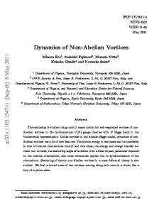
”out-of-plane” or ”non-planar” vortices which exhibit a localized structure of the Sz components around the vortex center. This structure falls off exponentially with a characteristic length, the vortex core radius [10] r 1 1−δ rv = , (1.2) 2 δ in units of the lattice constant a. The core radius increases with diminishing δ, allowing a continuous crossover to the isotropic Heisenberg model (δ = 0) where the topological excitations are merons and instantons [12], rather than vortices. Compared to the vortices in classical fluids [13] and superfluids [14], there is an important difference: The vortices of the easy-plane Heisenberg model carry two topological charges, instead of one: (1) The vorticity q = ±1, ±2, . . . which is defined in the usual way: The sum of changes of the azimuthal angle φ = arctan(Sy /Sx ) on an arbitrary closed contour around the vortex center yields 2πq; if the center is not inside the contour the sum is zero. In the following only the cases q = +1 (vortex) and q = −1 (antivortex) will be considered, the cases |q| > 1 would be relevant only for high temperatures. (2) The polarization or polarity p: For the non-planar vortices p = ±1 indicates to which side of the XY -plane the out-of-plane structure points, while p = 0 for the planar vortices (Fig. 1).

(a)

(b)

12 10 8 6 4 2 0 0

2

4

6

8

10

12

FIGURE 1. (a) In-plane structure of a static planar vortex (q = +1). (b) Out-of-plane structure of a static non-planar vortex with polarization p = +1.

Both topological charges 1 are crucial for the vortex dynamics, which is governed by two different forces: (1) 2D Coulomb-type forces F, which are 1

From the viewpoint of homotopy groups, q and Q = − 21 qp are π1 - and π2 topological charges, respectively; see Ref. [15].

4


proportional to the product of the vorticities of two vortices and inversely proportional to their distance (assuming that the distance is larger than 2rv , such that the out-of-plane structures do not overlap), (2) a ”gyrocoupling” force [16, 17] ˙ ×G FG = X (1.3) ˙ is the vortex velocity, and X(t) is the trajectory of the vortex where X center. The force (1.3) is formally equivalent to the Magnus force in fluid dynamics and to the Lorentz force on an electric charge. The gyrocoupling vector [18] G = 2πqp ez , (1.4) where ez is the unit vector in z-direction, does not represent an external field but is an intrinsic quantity, namely a kind of self-induced magnetic field which is produced by the localized Sz -structure and carried along by the vortex. For antiferromagnets G vanishes. Since the gyrovector (1.4) contains the product of both topological charges, the dynamics of the two kinds of vortices is completely different: (1) For planar vortices G = 0, therefore they have a Newtonian dynamics ¨ = F, MX

(1.5)

where the vortex mass M will be defined in section 2.2. However, in the simulations the trajectories are not smooth due to strong discreteness effects [19]. (2) Non-planar vortices have smooth trajectories if the diameter 2rv of the out-of-plane structure is considerably larger than the lattice constant [19]; i. e., if δ is not close to δc . For steady state motion, the dynamics is described by the Thiele equation [16, 17] ˙ × G = F, X

(1.6)

which was derived from the Landau-Lifshitz equation (section 2) for the spin vector Sm (t). This equation is identical to Hamilton’s equations with Hamiltonian (1.1). However, for arbitrary motion the Thiele equation (1.5) is only an approximation because a rigid vortex shape was assumed in the derivation. If a velocity dependence of the shape is allowed [20, 21], an inertial term ¨ appears on the l. h. s. of Eq. (1.6). However, this 2nd -order equation MX could not be confirmed by computer simulations [23, 24]. The reason will be discussed in section 2; in fact, a collective variable theory reveals that the dynamics of non-planar vortices can only be described by odd-order equations of motion. Therefore the dynamics is non-Newtonian. Another interesting topic is the dynamics under the influence of thermal fluctuations (section 3). Here white noise and damping are implemented in the Landau-Lifshitz equation. The same type of collective variable theory


5

as in section 2 then yields stochastic equations of motion for the vortices. The stochastic forces on the vortices can be calculated and the solutions of the equations of motion are compared with Langevin dynamics simulations. In this way, the diffusive vortex motion can be well understood. For somewhat higher temperatures (still below TKT ) the thermal noise can induce transitions of non-planar vortices from one polarization to the opposite one. Theoretical estimates of the transition rate are compared with Langevin dynamics simulations (section 3.3). For the temperature range above TKT , so far only a phenomenological theory exists, the vortex-gas approach (section 4). It contains only two free parameters (the density of free vortices and their r.m.s. velocity). The theory predicts ”central peaks” in the dynamic form factors for both inplane and out-of-plane spin correlations. Such peaks are observed both in computer simulations and in inelastic neutron scattering experiments, and many of the predicted features are confirmed. However, a recent direct observation of the vortex motion in Monte Carlo simulations has revealed that a basic assumption of the theory, namely a ballistic vortex motion, might not be valid. (In section 4 we confine ourselves to the ferromagnetic case, although easy-plane antiferromagnets were also investigated). The conclusion in section 5 will discuss the ingredients of a theory which can fully explain all observations above TKT .

2 Collective Variable Theories at Zero Temperature 2.1 Thiele Equation The spin dynamics is given by the Landau-Lifshitz equation, which is the classical limit of the Heisenberg equation of motion for the spin operator Sm , ∂H dSm (1.7) = −Sm × dt ∂Sm where H is the Hamiltonian, in our case that of the anisotropic Heisenberg model (1.1). The meaning of Eq. (1.7) is that the spin vector Sm pre∂H cesses in a local magnetic field B, with cartesian components Bα = − ∂S m. α In spin dynamics simulations (see below), the Landau-Lifshitz equation is integrated numerically for a large square lattice, typically with 72 × 72 lattice points. As initial condition a vortex is placed on the lattice and the trajectory X(t) of the vortex center is monitored. This trajectory is then compared with theory, i. e. with the solution of an equation of motion for the vortex. The standard procedure to obtain this equation consists in taking the continuum limit Sm (t) = S(r, t) where r is a vector in the XY plane, and in developing a collective variable theory.

6


The simplest version makes the travelling wave ansatz [16, 17] S(r, t) = S(r − X(t)) ,

(1.8)

where the functions Sα on the r. h. s. describe the vortex shape. (Strictly speaking, these functions should bear an index to distinguish them from the functions on the l. h. s.) As the equation of motion is expected to contain a force, the following operations are performed with Eq. (1.7) which yield force densities δH ∂S ∂S ∂S dS δH ∂H S = −S = −S 2 × × S× = −S 2 ∂Xi dt ∂Xi δS δS ∂Xi ∂Xi (1.9) with i = 1, 2 and Hamiltonian density H. According to the ansatz (1.8), dS ∂S ˙ Xj = dt ∂Xj

(1.10)

is inserted, with summation over repeated indices. Integration over r then yields the equation of motion ˙ = F, GX with the force Fi = −

Z

d2 r

(1.11)

∂H , ∂Xi

and the gyrocoupling tensor Z Z ∂S ∂S ∂φ ∂ψ ∂φ ∂ψ 2 2 Gij = d r S . × = d r − ∂Xi ∂Xj ∂Xi ∂Xj ∂Xj ∂Xi

(1.12)

(1.13)

The expression on the right was obtained by introducing the two canonical fields φ = arctan(Sy /Sx ), ψ = Sz (1.14) instead of the three spin components Sα with the constraint S = 1. The static vortex structure is [10] φ0 ψ0 ψ0

=

x′ q arctan ′2 x1 "

=

p 1−

=

r

pa2

a21

(1.15) r′ rv

2 #

rv −r′ /rv e r′

for r′ ≪ rv

for r′ ≫ rv

(1.16) (1.17)

where the constants a1 and a2 can be used for a matching, and r′ = r − X .

(1.18)


7

The integral then yields Gij = Gǫij , G = 2πqp

(1.19)

where ǫij is the antisymmetric tensor. Interestingly, only the value p of the Sz component at the vortex center enters the final result [18], i. e., the out-of-plane vortex structure needs not to be explicitly known here. As G is antisymmetric, Eq. (1.11) is identical to the Thiele equation (1.6) with gyrovector G = Gez . Since p = 0 and thus G = 0 for planar vortices, the Thiele equation is incomplete in this case. Obviously there must be a non-vanishing term on the l. h. s., this will be an inertial term (section 2.2). Moreover, the ansatz (1.8), and thus the Thiele equation, is only valid for steady-state motion when the vortex shape is rigid (in the moving frame). This includes not only translational motion with constant velocity V0 but also rotational motion with constant angular velocity ω0 . Both types of motion can be obtained by considering two non-planar vortices at a distance 2R0 which drive each other by their Coulomb force F = 2πq1 q2 /(2R0 ). For a certain velocity this force is compensated by the gyrocoupling force (1.3). In fact, since each vortex carries two charges, there are four physically different scenarios which represent stationary solutions of the Thiele equation. They fall into two classes: If the gyrovectors of the two vortices are parallel (i. e., q1 p1 = q2 p2 ), a vortex-vortex or vortex-antivortex pair rotates with ω0 on a circle with radius R0 around each other, where ω0 R02 =

1 q1 1 q2 = . 2 p1 2 p2

(1.20)

If the gyrovectors are antiparallel, the pair performs a parallel translational motion with velocity V0 and distance 2R0 , where V0 R0 = q2 /(2p1 ) = −q1 /(2p2 ). Both kinds of scenarios also appear for vortices in (super)fluids [13, 14]. However, in these contexts there are only two physically different situations: vortex-vortex rotation and vortex-antivortex translation.

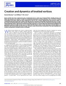
2.2 Vortex Mass The above scenarios for magnetic vortices were not tested by computer simulations until 1994, and the results were very surprising [22, 23]: Using a square or circular system with free boundary conditions, two of the four scenarios (vortex-vortex rotation and vortex-antivortex translation) were confirmed, but not the two other ones: For vortex-antivortex rotation and vortex-vortex translation the observed trajectories showed pronounced oscillations around the trajectories predicted by the Thiele equation (1.6) or (1.11), see Fig. 2. In fact, such oscillations had already been predicted [20, 21] by assuming that the vortex shape in the travelling wave ansatz (1.8) depends explicitely

8


20

0

−20 −20

0

20

FIGURE 2. Vortex-antivortex rotation on a circular system with radius L = 36 and free boundary conditions. Only the trajectory of the vortex center is plotted, the center of the antivortex is always opposite. The mean trajectory is a circle with radius R0 = 15.74.

˙ This leads to an additional term on the velocity X. and thus to an inertial term in the Thiele equation

∂S ˙j ∂X

¨ j in Eq. (1.10) X

¨ + GX ˙ = F, MX where M is the mass tensor ) ( Z Z ∂S ∂φ ∂ψ ∂φ ∂ψ ∂S 2 2 . × = d r − Mij = d r S ∂Xi ∂ X˙ j ∂Xi ∂ X˙ j ∂ X˙ j ∂Xi

(1.21)

(1.22)

This integral can be easily evaluated if the vortex is placed at the center of a circular system with radius L and free boundary conditions. The dominant contribution stems from the outer region ac ≤ r ≤ L, with ac ≃ 3rv , where the velocity dependent parts of the vortex structure are [10, 24] q (1.23) ψ1 = (x2 X˙ 1 − x1 X˙ 2 ) . 4δr2 (1.24) φ1 = p(x1 X˙ 1 + x2 X˙ 2 ) Together with the static parts φ0 from Eq. (1.15) and ψ0 , which falls off exponentially outside the core (1.2), the rest mass M is obtained Mij = M δij ,

M=

πq 2 L + CM . ln 4δ ac

(1.25)


9

The constant CM stems from the inner region 0 ≤ r ≤ ac , where the vortex structure is not well known due to the discreteness, but CM is not important for discussion. There is also a velocity dependent contribution to the mass which is negligible because the vortex velocities in the simulations are always much smaller than the spin wave velocity, which is the only characteristic velocity of the system. The above vortex mass is consistent with other results in the literature: Generalizing the momentum of solitons in 1D magnets [25], the vortex momentum Z P = − d2 r ψ∇φ (1.26)

is defined and can be shown to be a generator of translations [21]. Then ˙ results, but P is not a canonical momentum because the Poisson P = MX ˙ 2 /2 is bracket {P1 , P2 } = G does not vanish. For the kinetic energy M X obtained [10], therefore this energy and the rest energy E = π ln(L/ac )+CE both show the same logarithmic dependence on the system size L. For a continuum model of a 2D ferromagnet with uniaxial symmetry and a magnetostatic field, a slightly different vortex momentum was defined [26], namely Z PP T =

d2 r r × g ,

(1.27)

where g = ∇φ × ∇ψ represents the gyrovector density, cf. Eq. (1.13) which is related to the gyrovector as described below Eq. (1.19). The definition (1.27) depends on the choice of origin of the system and is not a generator of translations. Nevertheless, if the time derivative of PP T is set equal to the force F on the vortex, the generalized Thiele equation (1.21) is again obtained [21]. Therefore the vortex dynamics is qualitatively the same, as will be discussed now. Eq. (1.21) has the same form as that for an electric charge e in a plane with a perpendicular magnetic field B and an in-plane electric field E. I. e., the vortex motion is completely analogous to the Hall effect: The trajectory is a cycloid with frequency G ωc = , (1.28) M cf. the cyclotron frequency eB/(M c), where c is the speed of light. It is possible to transform to a frame where the force F vanishes and the vortex rotates (i. e., guiding center coordinates [27, 26, 21]). The cycloidal trajectories can explain qualitatively the oscillations observed in the simulations (Fig. 2). Moreover, the fact that oscillations are observed only for two of the four scenarios for two vortices (see above) can also be explained: A generalization of the ansatz (1.8) to the case of two vortices yields two coupled equations of motion with a 2-vortex mass tensor [28, 23]. In the case of vortex-vortex rotation and vortex-antivortex translation there are cancellations in this mass tensor which prevent oscillations, in agreement with the simulations.

10


However, a quantitative comparison of Eq. (1.21) and the simulations reveals two severe discrepancies [23, 24]: (1) The mass M = G/ωc which is obtained from Eq. (1.28) by inserting the observed frequency, turns out to be much larger than predicted by Eq. (1.25). Moreover, the dependence on the system size L is linear, while Eq. (1.25) predicts a logarithmic dependence. (2) Instead of the one frequency ωc of Eq. (1.28), two frequencies ω1,2 are observed in the spectrum of the oscillations (Fig. 3). As ω1 and ω2 are close to each other, a pronounced beat is observed in the trajectories (Fig. 2): The cycloidal frequency is (ω1 +ω2 )/2, but the shape of the cycloids changes slowly with (ω2 − ω1 )/2. 0.40 0.30 0.20 0.10 0.00 0.00

0.05

ω

0.10

0.15

0.10

0.15

0.030 0.025 0.020 0.015 0.010 0.005 0.000 0.00

0.05

ω

FIGURE 3. Upper panel: Fourier spectrum of the radial displacements r(t) = R(t) − R0 of the vortex in Fig. 2 from the mean trajectory; the integration time is 20000 in units (JS)−1 . Lower panel: Spectrum of the azimuthal displacements ϕ(t) = φ(t)−ω0 t from the mean trajectory, where ω0 is the angular velocity.

Both discrepancies have nothing to do with 2-vortex effects, because they also occur in 1-vortex simulations [24]. Here the vortex is driven by image


11

forces, in analogy to electrostatics. The most convenient geometry is a circular system with radius L and free boundaries. In this case there is only one image vortex which has opposite vorticity, but the same polarization [22, 29]. The radial coordinate of the image is L2 /R, where R is the vortex coordinate. The vortex trajectory can be fitted very well to a superposition of two cycloids. This observation will be explained in the next section.

2.3 Hierarchy of equations of motion Recently a very general collective variable theory was developed for nonlinear coherent excitations in classical systems with arbitrary Hamiltonians [24]. In this theory the dynamics of a single excitation is governed by a hierarchy of equations of motion for the excitation center X(t). The type of the excitation determines on which levels the hierarchy can be truncated consistently: ”Gyrotropic” excitations are governed by odd-order equations and thus do not have Newtonian dynamics, e. g. Galileo’s law is not valid. ”Non-gyrotropic” excitations are so-to-speak the normal case, because they are described by even-order equations, i. e. by Newton’s equation in the first approximation. Examples of the latter class are kinks in 1D models like the nonlinear Klein-Gordon family and the planar vortices of the 2D anisotropic Heisenberg model (1.1). The non-planar vortices of this model represent the simplest gyrotropic example. 3D models have not been considered so far. The basis fo the above collective variable theory is a ”generalized travelling wave ansatz” for the canonical fields in the Hamiltonian. For a spin system, as considered in this review, this ansatz reads ˙ X, ¨ . . . , X(n) ) . S(r, t) = S(r − X, X,

(1.29)

This generalization of the standard travelling wave ansatz (1.8) yields an (n + 1)th -order equation of motion for X(t), because Eq. (1.10) is replaced by dS ∂S ¨ ∂S ˙ ∂S (n+1) Xj + = . (1.30) X Xj + · · · + (n) j ˙ dt ∂Xj ∂ Xj ∂X j

The same procedure as described below Eq. (1.10) then yields the (n+1)th order equation. The case n = 1 corresponds to the 2nd -order equation (1.21). In one dimension the antisymmetric tensor G from Eq. (1.13) vanishes and (1.21) reduces to a Newtonian equation. The same is true for the 2D planar vortices where Gij = 0 because p = 0 in Eq. (1.19). The case n = 2 yields the 3rd -order equation ... ¨ + GX ˙ = F(X) AX + MX

(1.31)

12


with the 3rd -order gyrotensor Aij =

Z

∂S ∂S d rS × = ¨j ∂Xi ∂ X 2

Z

2

d r

(

∂φ ∂ψ ∂φ ∂ψ − ¨ ¨ j ∂Xi ∂Xi ∂ Xj ∂X

)

.

(1.32)

For the above 1D models and the 2D planar vortices nothing changes because Aij turns out to be zero (below). But the 2D non-planar vortices are the first gyrotropic example. For the calculation of the integral (1.32) the acceleration dependence of the outer region of the vortex is needed [24] ψ2 =

p ¨2) ¨ 1 + x2 X (x1 X 4δ

q ¨ 2 ) ln r . ¨ 1 − x1 X (x2 X 8δ eL Together with the static parts φ0 and ψ0 this yields φ2 =

Aij = Aǫij ,

A=

G L2 − a2c + CA , 16δ

(1.33) (1.34)

(1.35)

where the constant CA stems from the inner region. In the simulations the dynamic in-plane structures φ1 and φ2 cannot be clearly observed because it is difficult to subtract the static structure φ0 which varies drastically with the vortex position. However, the dynamic out-of-plane structures ψ1 and ψ2 can be observed and distinguished by looking at specific points of the trajectory: E. g., at the turning points in Fig. 4 the acceleration is maximal while the velocity is small. Figs. 5, 6 confirm the structure of ψ2 in the outer region, they also show that this structure oscillates as a whole, with frequency (ω1 + ω2 )/2. An alternative interpretation of this oscillating structure in terms of certain ”quasilocal” spinwaves will be given in section 2.4. ¨ j and as Aij contains derivatives with As ψ2 and φ2 depend linearly on X ¨ j , the leading contribution to Aij is independent of velocity and respect to X acceleration. There are higher-order terms which are negligible, though; cf. the discussion of the mass. For these reasons the l. h. s. of the equation of motion (1.31) is linear. The radial Coulomb force F on the r. h. s. can be linerarized by expanding in the small radial displacement r(t) = R(t) − R0 from the mean trajectory which is a circle of radius R0 F (R) = F (R0 ) + F ′ (R0 )r .

(1.36)

The 3rd -order equation of motion (1.31) then has the following solutions [24]: A stationary solution and a superposition of two cycloids r(t)

=

R0 ϕ(t) =

a1 cos ω1 t + a2 cos ω2 t b1 sin ω1 t + b2 sin ω2 t

(1.37)


13

12.4

R

12.2

12.0

11.8

0

5

10

R0φ

15

20

25

FIGURE 4. First part of the trajectory of a vortex with q = p = 1 on a circular system with radius L = 36 and free boundary conditions. The small diamonds (⋄) mark the position of the vortex in time intervals of 10(JS)−1 .

where ϕ = φ − ωo t is the azimuthal displacement. The results for ω1,2 can be considerably simplified for R0 ≪ L, which is the case in the simulations. The frequencies ω1,2 form a weakly-split doublet. The mean frequency depends on A, but not on M : p √ ω ¯ = ω1 ω2 = G/A ∼ 1/L (1.38) for large L. Contrary to this, the splitting of the doublet ∆ω = ω2 − ω1 = M/A ∼

ln L L2

(1.39)

is proportional to the mass. As G = 2πqp is known from Eq. (1.19), the last two equations are sufficient to determine M and A by using the frequencies ω1,2 observed in the simulations. In Ref. [24] the data for lattice sizes L = 24 . . . 72 were extrapolated for R0 → 0 by using several runs for small R0 /L, because the theoretical predictions (1.25) and (1.35) were made for R0 = 0. For the

14


FIGURE 5. Out-of-plane structure of the vortex at the 7th turning point of the trajectory in Fig. 4. Here the acceleration has a maximum and points in the radial direction, while the velocity is small and points in the azimuthal direction.

anisotropy δ = 0.1 the data for A are well represented by A = CLα + A0 with α = 2.002, C = 4.67 and A0 = 40. This agrees rather well with the L2 -term in (1.35), the constant CA cannot be tested. However, M ≈ 15 is nearly independent of L, in contrast to the logarithmic dependence in Eq. (1.25). This can be connected to the observation that the velocity dependent part ψ1 seems to approach an L-independent constant at the boundary, in contrast to the predicted 1/r-decay in Eq. (1.23). A very interesting point is the discussion of the size dependence of the different terms in the equation of motion (1.31). As every time derivative of Xi contributes a factor of ω1,2 = O(1/L), the orders of the terms are ... ¨ i = O(ln L/L2) and GX˙ i = O(1/L). Therefore the A X i = O(1/L), M X rd strong 3 -order term cannot be neglected when the weak 2nd -order term is retained. This is the reason for the two severe discrepancies between the simulations and the predictions of the 2nd -order equation (1.21), which were discussed in section 2.2. However, the neglection of both the 2nd - and 3rd -order terms represents a consistent first approximation, namely, the Thiele equation (1.11). The next consistent approximation in the hierarchy is the 3rd -order equation (1.31), as discussed above. An investigation of even higher-order terms in Ref. [24] confirms the conjecture that only the odd-order equations of the hierarchy represent valid approximations for gyrotropic excitations (For


15

FIGURE 6. Same as in Fig. 5, but at the 8th turning point, where the accelaration points in the negative radial direction.

non-gyrotropic ones all members of the hierarchy are even). The odd higher-order equations predict additional frequency doublets ω3,4 , ω5,6 etc. These frequencies normally vanish in the background of the spectrum. However, they become visible if the simulations are specially designed: For a vortex in the center of a quadratic system with antiperiodic boundary conditions, all image forces cancel exactly and only the small pinning forces remain. For this configuration two additional doublets with strongly decaying amplitudes were indeed observed [24]. Finally we mention that cycloidal vortex trajectories have been found not only in field-theoretic models for magnets [26, 30], but also for (1) neutral and (2) charged superfluids: (1) In the Ginzburg-Landau theory, which describes vortex motion in thin, neutral, superfluid films, the usual assumption of incompressibility was dropped [31]. A moving vortex then exhibits a density profile in the region outside the vortex core. This profile is similar to the velocity dependent outof-plane structure (1.23) of the magnetic vortices, and the consequences are also similar: There are small-amplitude cycloids [32] superimposed on the trajectories in both 2-vortex scenarios (vortex-vortex rotation and vortexantivortex translation, see end of section 2.1). (2) For the dynamics of vortices in a charged superfluid the same kind of superimposed cycloids was found, again for both 2-vortex scenarios [33]. Here a field-theoretic model was used, where a charged scalar field is min-

16


imally coupled to an electromagnetic field and a φ4 -potential is included; this is proposed as a phenomenological model for a superconductor. However, compared to the dynamics of magnetic vortices as reviewed in this article, there is an important difference: For all the models discussed above, there is only one cycloidal frequency; correspondingly the vortex dynamics is governed by 2nd -order equations of motion. It will be interesting to study many other physical contexts in which topological vortex structures appear (e. g., dislocations in solids and flux lattices, vortex filaments in compressable fluids and complex GinzburgLandau models). We expect that the details of the vortex dynamics differ, depending on the order of the equations of motion, for instance (see beginning of this section).

2.4 An alternative approach: Coupling to magnons The spirit of the generalized travelling wave ansatz (1.29) differs considerably from the well-known standard ansatz, which reads for a spin system S(r, t) = S0 (r − X(t)) + χ(r, t) .

(1.40)

Here S0 represents the static structure of a single nonlinear coherent excitation (a vortex in our case) and χ represents a magnon field (or meson field for other kinds of systems). Since S0 is static, but the shape of the excitation usually depends on the velocity, a part of the dynamics obviously must be taken over by the spin waves. Based on earlier work, this concept has very recently been carried through [40]. First, the magnon modes in the presence of a single static vortex were obtained by a numerical diagonalization for relatively small, discrete systems with fixed (Dirichlet) boundary conditions (BC) [34, 35, 36]. Analytical investigations were done for planar vortices in antiferromagnets [37, 39] and ferromagnets [38, 39]. These articles demonstrated nontrivial properties of the eigenmodes, e. g., the presence of quasi-local (resonance type) [34, 35] or truly local [36] modes. Moreover, the relevance of these modes for the vortex dynamics was shown, in particular the transition between planar and non-planar vortices was investigated [34, 35]. However, for non-planar vortices all this was based on numerical diagonalization. But very recently, a general theory of vortex-magnon coupling was developed for arbitrarily large systems with circular symmetry and general BC [40]. The S-matrix for vortex-magnon scattering was calculated and expressed by Bessel and Neumann functions. Using the S-matrix, general formulas for the eigenfrequencies were obtained, as a function of the parameters and size of the system, and for different BC, namely for Dirichlet (fixed) and von Neumann (free) BC. There is a very good agreement between the frequencies of the two lowest quasi-local modes and the frequencies ω1,2 , which were observed for the


17

vortex trajectories in spin dynamics simulations for the discrete system √ (section (2.2). The error is only 0.8 % for the mean frequency ω ¯ = ω1 ω2 and 4 % for the splitting ∆ω = ω2 − ω1 . This demonstrates very clearly that the cycloidal vortex motion is accompanied by certain magnon modes, namely by quasi-local modes. These modes are both extended (like the other magnon modes) and local, because they exhibit a localized structure around the vortex center (Fig. 7). The structure of these modes is qualitatively similar to the dynamic vortex structure, which oscillates with the rythm of the cycloidal motion (Figs. 5, 6). However, only the out-of-plane part ψ of this structure can be clearly observed, and only in the outer region (see section 2.3).

FIGURE 7. One of the two low-lying quasi-local spin wave modes in a complex representation, obtained by a numerical diagonalization for a circular system with a vortex in its center, from [29] (In this reference m corresponds to our ψ).

As the frequencies ω1,2 in the cycloidal vortex motion are the same as the frequencies of the lowest quasi-local modes, and as the latter ones were

18


calculated analytically, the parameters A and M in the 3rd -order equation of motion (1.31) can also be calculated analytically [40]. The results can be expressed by the first root x1 of the equation aJ1 (x) + bxJ1′ (x)rv /L = 0, where J1 is a Bessel function. The values for a and b define the boundary conditions: a = 0, b = 1 for free BC and vice versa for fixed BC. The general result π L2 (1.41) A= 2δx21 in the limit of large L specializes to A = 4.634L2 for δ = 0.1 and free BC, which agrees perfectly with the result 4.67L2.002 from the simulations (section 2.3). For fixed BC A = 1.07L2 is about four times smaller. The general result for the vortex mass M is much more complicated than Eq. (1.41) and can be found in Ref. [40]. The numerical value M = 14.74 for δ = 0.1 and free BC agrees well with the value 15 from the simulations (section 2.3). However, both results are independent of the system size L, in contrast to the logarithmic L-dependence (1.25) predicted by the integral (1.22) in the collective variable theory, cf. the discussion in section 2.3. For fixed BC, M = 7.661 is obtained, about half of the above value for free BC. The fact that both the mass M and the factor A in the 3rd -order gyrocoupling term depend strongly on the boundary conditions appears very natural because the vortices are not localized excitations like solitons in 1D; the in-plane vortex structure falls off with 1/r. It is important to note that the higher-lying quasi-local modes could be calculated by the same methods, and are expected to agree with the higherorder doublets ω3,4 , ω5,6 , . . . appearing in the spectrum of the trajectories. Each additional doublet corresponds to taking into account two additional orders in the generalized travelling wave ansatz (1.29), as discussed in section 2.3. Finally, we mention the recent development of a very general collective variable theory for an arbitrary Hamiltonian H[φ, ψ] supporting nonlinear coherent excitations, without making any approximations [29, 41]. This theory starts with the standard ansatz for φ(r, t) and ψ(r, t), cf. Eq. (1.40), but imposes constraints between the meson fields and the functions φ0 (r; X1 , . . . , Xm ) and ψ0 (r; X1 , . . . , Xm ), which describe the shape of the excitation. Here the Xi (t) are m collective variables for the position and the internal modes of the excitation (if there are any). There are then 2m constraints in order to preserve the correct number of degrees of freedom. Consequently, the mathematical formalism is based on the classical limit of Dirac’s quantum mechanics for constraint systems. The equations of motion for the collective variables are a generalization of Thiele’s equation (1.11). The rank of the gyrocoupling matrix G is used to classify the excitations: In the case of vanishing G the excitations have an effective mass and exhibit Newtonian dynamics; in the case of regular G, the excitations behave like charged, massless particles in an external magnetic field, similar to the gyrotropic excitations defined in section 2.3. The above


19

theory is a generalization of earlier work of Tomboulis [42], Boesch et al. [43], and Willis et al. [44], which applies only to “standard” Hamiltonians (i. e., consisting of the sum of kinetic and potential energy terms). This generalization is necessary, e. g., in the case of magnetic systems which cannot be modelled by standard Hamiltonians.

3 Effects of thermal noise on vortex dynamics 3.1 Equilibrium and non-equilibrium situations As already mentioned in the introduction, below TKT vortex-antivortex pairs appear and vanish spontaneously due to thermal fluctuations. But these pairs do not move and therefore give no contribution to the dynamic correlation functions. Above TKT , some of the pairs unbind and the free vortices can move. In section 4, this situation will be investigated by a phenomenological theory, namely the vortex gas approach. On the other hand, the effect of thermal fluctuations on single vortices can be studied by putting a vortex in a thermal bath. This is a non-equilibrium situation, in fact it takes a long time until equilibrium is reached: The vortex very slowly approaches the boundary where it annihilates together with an image antivortex; during this process spin waves are radiated which are eventually thermalized. The vortex motion with thermal noise is a random walk process, where a vortex diffusion constant can be defined. This offers the possibility to develop an ab-initio theory for the dynamic form factors. This can be compared with the phenomenological vortex gas approach, which assumes, however, a ballistic motion (section 4).

3.2 Collective variable theory and Langevin dynamics simulations In principle, the generalization of a collective variable theory to finite temperatures is a straightforward procedure consisting of 4 steps: (1) Thermal noise and damping (because of the fluctuation-dissipation theorem) are introduced into the microscopic equations. (2) A travelling wave ansatz for a nonlinear coherent excitation is made which yields equations of motion with stochastic forces acting on the excitation. (3) The solutions of these stochastic o. d. e.’s are used to calculate the variances of the trajectory, which contain as a factor an effective diffusion constant for this excitation. The dependences of this constant on the temperature and other parameters can be discussed. (4) The predicted variances and the effective diffusion constant are com-

20


pared with the same quantities as observed in Langevin dynamics simulations. Step 1: Introduction of thermal noise This step is very problematical, although there are many papers in which the problems are either not appreciated or hidden. There are basically two major problems: (a) The microscopic equations can often be written in different ways which are equivalent. In the case of spin systems, the Landau-Lifshitz equation for the spin S is equivalent to the Hamilton equations for φ and ψ. However, if noise is implemented, e. g., by an additive term, the results may be qualitatively different (see below). (b) Typically, either additive or multiplicative noise can be used, but many papers do not give a reason why one of the two types was chosen. However, the results are usually qualitatively different for the two types of noise. In the case of the vortex dynamics, both major problems have been investigated in a preprint [45]: Additive noise in the Hamilton equations yields a vortex diffusion constant DV which depends logarithmically on the system size, while in the multiplicative case DV is independent of the system size. Additive noise in the Landau-Lifshitz equation [46, 47] yields a diffusion constant with the same logarithmic term as in the case of additive noise in the Hamilton equations, but the small constants that appear in addition to the logarithmic term differ for the two cases because the vortex core gives different contributions. Unfortunately, the additive noise in the Landau-Lifshitz equation has an unphysical feature, namely the spin length is not conserved. In the collective variable theory this problem is overcome by a constraint, while in the simulations a renormalization of the spin length is necessary after every time step2 . However, taking additive noise and using these little tricks is not really necessary, because there is a better noise term which eventually leads to the same results, but which is well motivated on physical grounds and which conserves the spin length [45, 48]: In the Landau-Lifshitz equation (1.7) each spin Sm precesses in a local magnetic field B which is the gradient of the energy with respect to the spin compononts. This local field is the only way through which the spin Sm can feel any changes in its environment. Adding a thermal noise term to the local field thus accounts for the interaction of the spin with magnons, phonons and any other thermally generated excitations. The stochastic Landau-Lifshitz equation then reads

2

Technically, this is achieved by adding a Lagrange parameter multiplying the constraint [46]. This means that a multiplicative noise term appears besides the additive one.


dSm dSm ∂H m m m + h (t) − ǫS × = −S × . dt ∂Sm dt

21

(1.42)

Because of the cross product with Sm this noise is multiplicative. In Ref. [45] Gaussian white noise is used:

=

0

(1.43)

> =

Dδ mn δαβ δ(t − t′ ) ,

(1.44)

where D = 2ǫkB T is the diffusion constant and α, β denote cartesian components. Following Refs. [16, 17, 18], a Gilbert damping with damping parameter ǫ was chosen in Eq. (1.42), chiefly because it is isotropic, in contrast to the Landau-Lifshitz damping [49]. Strictly speaking, the three equations (1.42) do not really represent Langevin equations, because all the components of dSm /dt appear in each equation due to the cross product. To properly introduce the noise, one first has to group all the time derivatives on the l. h. s. of the equation, and only then one can introduce independent white noise terms for each spin component. But this procedure eventually produces only a renormalization of the damping parameter ǫ in the order of ǫ2 . In the simulations values of ǫ in the order of 10−3 were used, and therefore the correction factor can even be neglected. Another, even more important issue is the interpretation of the stochastic differential equation (1.42). As the noise is multiplicative, Ito and Stratonovi˘c interpretations do not coincide, in contrast to the additive noise case [50, 51]. In principle, when thinking of thermal excitations interacting with the spins, there would be a finite correlation time which would lead to a colored noise term. Taking white noise means taking the limit of zero correlation time, and therefore the stochastic Landau-Lifshitz equation (1.42) must be interpreted in the Stratonovi˘c sense. As noted in the beginning of this subsection, the remaining three steps of the stated procedure are straightforward. Therefore we present here only the results for the case of non-planar vortices. Step 2: Stochastic equation of motion The generalized travelling wave ansatz (1.29) up to order n = 2 yields the 3rd -order stochastic o. d. e. ... ¨ + GX ˙ = F(X) + Fmult (t) (1.45) AX + MX The tensors A, M and G are the same as in Eqs. (1.19), (1.25) and (1.35), except that all the vanishing components in these three expressions are now replaced by damping terms proportional to ǫ. Thus the damping appears at every order in Eq. (1.45). Without Fmult , the solution is obtained in complete analogy to section 2.3: Two cycloids are superimposed on an

22


outward spiral on a circle (Fig. 8). In the simulations the purpose of the damping is to dissipate the energy which is supplied to the system by the kicks of the noise. Therefore the range of ǫ (for a given system size L) must be determined in which the cycloidal frequencies ω1,2 in the trajectories are not influenced by the damping [46]. The result is the condition ǫL ≪ 6.

FIGURE 8. Schematic sketch of the vortex motion as governed by the Landau-Lifshitz equation with Gilbert damping. The plot is approximate and does not correspond to an actual simulation.

The stochastic force in (1.45) Fimult (t) =

1 S2

Z

d2 r

∂S h(r, t) , ∂Xi

(1.46)

which stems from the multiplicative noise in Eq. (1.42), has zero mean and the correlation function [45] Z ∂S ∂S < Fimult (t)Fjmult (t′ ) >= Dδij δ(t − t′ ) d2 r . (1.47) ∂Xi ∂Xj Putting the vortex on the center of a circular system of radius L with free BC, the leading contribution to the variance is obtained [47] by using the static vortex structure (1.15) to (1.17) (1.48) Var Fist = DV δ(t − t′ ) with the vortex diffusion constant

L DV = Dπ ln +C , ac

(1.49)


23

here C stems from the inner vortex region 0 ≤ r ≤ ac and is obtained by numerical integration [47]. The variance (1.48) is a remarkable result for two reasons: (a) The stochastic forces acting on the vortex represent additive white noise with an effective diffusion constant. The point is that this was shown by going from the microscopic level, where multiplicative white noise was implemented, to the level of the collective variables. This approach is much more satisfying than assuming ad hoc a noise term on the collective variable level. (b) The mean and variance of the stochastic force (1.46) turn out to be the same as those of the stochastic force Z 1 ∂S add 2 Fi = 2 d r S × η(r, t) , (1.50) S ∂Xi which resulted from starting with additive white noise η(r, t) in the LandauLifshitz equation; this noise has already been discussed in step 1. This equivalence of the two forces means that in the case of the vortices additive noise and the multiplicative noise in Eq. (1.42) have the same effect on the vortex dynamics. This is a nontrivial result, because normally a qualitative difference is expected (cf. the discussion in step 1). Qualitatively, this result can be understood by noting that the renormalization of the spin length in the case of additive noise introduces effectively a multiplicative noise term, in addition to the additive one (cf. footnote in step 1). Step 3: Variances of the vortex trajectory The inhomogeneous stochastic 3rd -order o. d. e. (1.45) can be solved [47] by a standard Green’s function formalism, because the l. h. s. is linear and the deterministic force F(X) on the r. h. s. can be linearized by expanding in the displacement x(t) = X(t)− X0 (t) from the mean trajectory X0 (t) on which the vortex is driven by F, cf. Eq. (1.36). Knowing x(t), the variance matrix 2 σij (t) = hxi xj i − hxi ihxj i. (1.51) can be calculated; here i, j denote polar coordinates R and φ. Each element of the matrix (1.51) turns out to consist of 36 terms. In order to facilitate the discussion several simplifications can be made which give the following results [47]: 1 2 −βt 1 −2βt DV −2βt 2 t+ (1 − e )− e sin ω ¯t + e sin 2¯ ωt σRR (t) = (2π)2 4β ω ¯ 4¯ ω (1.52) √ with ω ¯ = ω1 ω2 and β ≃ ǫ/5 is the damping constant for the vortex motion. For large times, t ≫ 1/β, only the first term remains and the variance is linear in time, the standard random walk result. Interestingly, this result is identical to the one which is obtained by omitting the 2nd - and 3rd -order

24


terms in the stochastic equation of motion (1.45). This obviously means that these two terms have the following effects: (a) They produce the oscillatory parts in Eq. (1.52), which are naturally connected to the cycloidal oscillations in the vortex trajectories, 2 (b) for small times, t ≫ 1/β, the slope of σRR , averaged over the oscillations, is larger by a factor of 3/2 compared to late times. However, the first effect cannot be observed in the simulations because the oscillations are hidden in strong discreteness effects (see next step). For this reason we discuss only the long-time behavior of the other elements of the variance matrix 2 σRφ (t)

=

2 σφφ (t)

=

1 DV kF0′ 2 t 2 (2π)2 2π " 2 # DV 1 kF0′ t+ t3 (2π)2 3 2π

(1.53) (1.54)

with k = 1 − F0 /(F0′ R0 ) and F0 = F (R0 ), F0′ = F ′ (R0 ). The quadratic and cubic time dependences are non-standard results which appear in addition to the standard linear dependence because the deterministic force field F (R) = F0 + F0′ (R − R0 ) is inhomogeneous. F is a radial force which drives the vortex in the azimuthal direction, due do the gyrocoupling force (1.3). 2 Therefore, only the φ-components of σ 2 are affected: σRφ acquires a factor ′ 2 kF0 /(2π) · t, while σφφ acquires it twice. Step 4: Langevin dynamics simulations The stochastic Landau-Lifshitz equation (1.42) was solved numerically for a large circular lattice with free BC and one vortex driven by a radial image force [45, 46, 47]. The mean trajectory is an outward spiral. Therefore a small damping parameter ǫ was chosen in order to allow long integration times. There are several qualitatively distinct temperature regimes. For 0 ≤ T < T3 ≈ 0.05 (in dimensionless units, where TKT ≈ 0.70 for the XY-model [52, 53]), two frequencies are observed in the oscillations around the mean trajectory which can be identified with the cycloidal frequencies ω1,2 in section 2.3. As these frequencies are constant in the whole regime, the 3rd order equation of motion (1.45) with temperature independent parameters can in fact describe the vortex dynamics. For T3 < T < T1 ≈ 0.3 the above two frequencies cannot be observed any longer due to large fluctuations , thus the 1st -order equation of motion is sufficient here. However, in some of the runs the vortex suddenly changed its direction of motion; this will be explained in the next subsection. Finally, for T > T1 , a single vortex theory is no longer adequate because here the probability for the spontaneous appearance of vortex-antivortex pairs in the neighborhood of the single vortex becomes too large.


25

DV

1.00

0.10

0.01

0.001

0.010 T

FIGURE 9. Vortex diffusion constant DV as a function of temperature, for ǫ = 0.002 and L = 24. Solid line: Theoretical results from Eq. (1.49); dashed line: Adjusted DV from fitting the theoretical curves for σ 2 (t) to the simulation data.

The linear, quadratic, and cubic time dependences in Eqs. (1.52) - (1.54) are well confirmed by the simulations. Therefore the factor DV can be fitted and turns out to differ from the predicted vortex diffusion constant (1.49) only by a nearly temperature independent factor of about 1.8, see Fig. 9 (The constant C in (1.49) was obtained by a numerical integration over the vortex core [46]). This agreement is amazingly good, taking into account that the simulations were performed for a discrete lattice while the theory works in the continuum limit and uses additional approximations, like the expansion (1.36) of the Coulomb force.

0.012 0.010

σ2RR

0.008 0.006 0.004 0.002 0.000 -0.002 0

200

400

600

800

1000

t

FIGURE 10. Variance of the radial vortex coordinate averaged over 2000 realizations, for T = 0.003, ǫ = 0.002, and L = 24. The dashed vertical lines indicate the times at which the vortex center moves over ridges of the Peierls-Nabarro periodic potential.

26


Although discreteness effects are hardly visible in the trajectories of nonplanar vortices at zero temperature [19], see also Fig. 2, these effects are very important at finite temperatures: Fig. 10 clearly demonstrates that the variance of the trajectory shows a pronounced peak whenever the vortex center moves over a ridge of the Peierls-Nabarro potential. Due to this effect, the predicted cycloidal oscillations (1.52) in the variance cannot be observed.

3.3 Noise-induced transitions between opposite polarizations As already mentioned above, a vortex in a thermal bath can suddenly change its direction of motion on its outward spiral. A closer inspection shows that this occurs because, opposite to the vorticity q, the polarization p is not a constant of motion for a discrete system: The out-of-plane vortex structure can flip to the other side of the lattice plane due to the stochastic forces acting on the core spins. Then the direction of the gyrovector (1.4) is reversed and according to the Thiele equation (1.6) the direction of motion is reversed as well (The same holds for the 3rd -order equation (1.31) because A ∼ G in Eq. (1.35)). In a preprint [54] the cores of both planar and non-planar vortices are described by a discrete Hamiltonian, similar to the one which was used for the study of the instability at δ = δc [34, 11]. Using the stochastic Landau-Lifshitz equation (1.42) the Fokker-Planck equation is derived. Its stationary solution exhibits two maxima for the two possible polarizations of the non-planar vortex and a saddle point for the planar vortex, if the anisotropy parameter δ lies in a certain temperature dependent range. The rate κ for the transition from one polarization to the opposite one is calculated in analogy to Langer’s instanton theory [55, 56], using the fact that for δ → δc there is a soft mode among the normal modes which were obtained numerically for a system with one vortex [35]. Taking into account only the four innermost spins of the core, a very simple result is obtained κ=

1 p − ∆E (1 − δ)2 − (1 − δc )2 e kB T 2π

(1.55)

where ∆E is the energy difference between the planar and the non-planar vortex. For δ = 0.1, the average transition times τ = κ−1 are 100440, 4837, and 1060 for T = 0.1, 0.15, and 0.2 respectively. Despite of the crude model for the vortex core, these values agree rather well with the transition times from Langevin dynamics simulations: τ = 92516, 4016, and 825 for the above temperatures, with statistical errors of 22%, 6%, and 10%, respectively.

This is page 27 Printer: Opaque this

4 Dynamics above the Kosterlitz-Thouless transition 4.1 Vortex-gas approach This is a phenomenological theory which is based on the following assumptions: Above TKT , the free vortices form a dilute gas and move either diffusively [57, 58, 18] or ballistically [59]. In the former case, only spin autocorrelation functions were calculated which lead to dynamic form factors without wavevector dependence. Therefore we review only the latter case [59]: The density nv and the r. m. s. velocity v are the only free parameters. According to Kosterlitz and Thouless [6] nv ≈

1 , (2ξ)2

(1.56)

where ξ is the static spin correlation length which diverges with an essential singularity for T → TKT from above. Therefore the vortex gas is in fact dilute if T is close enough to TKT . The vortex density is homogeneous only on the average, locally the distribution is expected to be random. Therefore the net force is zero on the average and the distribution around zero is Gaussian, which yields a Maxwellian velocity distribution. This also holds for the non-planar vortices because the velocity is proportional to the cross product of the net force and the gyrovector, due to the Thiele equation (1.6). However, the assumption of a ballistic vortex motion is problematic (section 4.3). Under this assumption the dynamic spin-spin correlation functions Sαα (r, t) = hSα (r, t)Sα (0, 0)i , α = x, y, z , (1.57) and their space-time Fourier transforms, namely the dynamic form factors Sαα (q, ω), can be calculated analytically [59]. There is an important difference between in-plane correlations (α = x, y) and out-of-plane ones (α = z): As the in-plane vortex structure is not localized (it has no spatial Fourier transform), Sxx = Syy are only globally sensitive to the presence of the vortices and the characteristic length scale is their average distance 2ξ. The dynamic form factor exhibits a “central peak”, i. e. a peak around ω = 0, with the (squared) Lorentzian form Sxx (q, ω) =

1 γ 3ξ2 , 2π 2 ω 2 + γ 2 [1 + (ξq)2 ]2

(1.58)

√ where γ = πv/(2ξ). Here the core structure did not enter the result, because the theory was worked out on a length scale much larger than the core radius rv . The integrated intensity Ix (q) of (1.58) is inversely

28


proportional to the density nv , therefore the motion of the vortices actually destroys correlations. For the out-of-plane correlations Szz the situation is completely different: The non-planar vortices have statically the localized Sz structure (1.16), (1.17) which has a spatial Fourier transform, namely the static form factor f (q). Therefore Szz is locally sensitive to the vortices, i. e., to their size and shape. Consequently nv |f (q)|2 ω2 Szz (q, ω) = (1.59) exp − (vq)2 4π 5/2 v q contains f (q) and is proportional to the density. This Gaussian central peak simply reflects the Maxwellian velocity distribution. For the planar vortices the situation is more complicated because they do not have a static Sz structure but only a dynamic one, namely Eqs. (1.23), (1.24). Therefore the form factor is velocity dependent which yields a more complicated result for Szz [10], containing the same Gausssian as in Eq. (1.59). However, the intensity of this peak is much smaller than that of the peak (1.59), because the dynamic Sz components are about two orders of magnitude smaller than the static ones [24].

4.2 Comparison with simulations and experiments In combined Monte-Carlo (MC) and Spin Dynamics (SD) simulations many features of the predicted dynamic form factors (1.58) and (1.59) were confirmed: (1) In-plane correlations: Both for the XY-model (δ = 1) [59] and for the weakly anisotropic case (δ < δc ) [60], the observed Sxx (q, ω) exhibits a central peak for T > TKT (but not for T < TKT , as expected). The statistical errors were too large to decide about the shape. However, the width Γx (q) and the integrated intensity Ix (q) of the Lorentzian (1.58) can be fitted to the data, in this way the free parameters ξ and v are determined. ξ(T ) agrees rather well with the static correlation length [6]. v(T ) increases with T and then saturates; except of a factor of about 2, this agrees with a result of Huber [58, 18] who assumed a diffusive vortex motion and calculated the velocity autocorrelation function. Central peaks were also observed in inelastic neutron scattering experiments: For BaCo2 (AsO4 )2 [61] and Rb2 CrCl4 [62] the measurement was performed for only a few q-values. The reported widths of the peaks differ from the predicted Γx (q) by factors of about 7 and 2.5, resp.. However, in this comparison one has to take into account that the theory has neglected many features of the real quasi-2D materials: E. g., the lattice structure, a pronounced in-plane anisotropy in the case of BaCo2 (AsO4 )2 , and quantum effects. For CoCl2 graphite intercalation compounds the q-dependence of the


29

central peak width was measured [2] and agrees qualitatively with Γx (q) from the peak (1.58). (2) Out-of-plane correlations: In MC-SD simulations, Szz (q, ω) exhibits a central peak only together with a spin wave peak which sits on its shoulder (in contrast to Sxx where the spin waves are strongly softened for small q). For the XY-model (δ = 1), which bears planar vortices, the intensity of the central peak is expected to be small (see end of section 4.1). Early simulations with large statistical errors [10] had difficulties to substract the spin wave peak and reported only upper bounds for the width Γz (q) and the intensity Iz (q) of the central peak. Recent simulations with much better statistics investigated the range δc < δ ≤ 1. Some papers did not find a central peak [63, 53] others did [64]. However, for the weakly anisotropic case (δ < δc ) with non-planar vortices a central peak was indeed found [63]. Experimentally, Szz (q, ω) was first not accessible because of intensity problems. Only the use of spinpolarized neutron beams made it possible to observe a central peak in Rb2 CrCl4 and to distinguish it from the spin wave peak and from other contributions [65]. The measured width is practically equal to the width of the Gaussian (1.59). However, such a good agreement seems to be accidental because this material exhibits a breaking of the rotational symmetry in the XY-plane which is described by a more complicated Hamiltonian [66]. For the same reason it is not clear whether this material actually belongs to the case δ < δc .

4.3 Vortex motion in Monte Carlo simulations The vortex gas approach assumes for single free vortices a diffusive [57, 58] or ballistic [59] motion. Very recently this was tested in MC-simulations by monitoring the position of each vortex in the system (free or bound in a pair) as a function of time [67, 68, 69]. The surprising result is that a single vortex very seldom moves freely over a larger distance. Normally the vortex travels only one or a few lattice spacings until it annihilates with the antivortex of a pair which meanwhile appeared spontaneously in the neighborhood. Another possibility is that the single vortex docks on a pair or a cluster of pairs and after a while one of the vortices leaves the cluster. These results confirm suggestions that vortices cannot move freely for more than a few lattice spacings, which were made by computing the vortex density-density correlation function [70, 67]. However, the interpretation of these results is not clear at all. One possibility is that the vortex gas approach is not valid [67, 68], but then the striking qualitative agreement with the central peaks in the simulations and experiments is not understood. We favour another possibility: Probably only the effective vortex motion is important for the dynamic correlation function Sxx (r, t) (1.57). This would mean that it does not matter if a vortex is annihilated with the antivortex of a pair in the considered time

30


interval [0, t], because the vortex of that pair continues the travel instead of the original vortex. Only effective lifetimes are seriously affected. This picture is strongly supported by the mechanism [59] which yields the central peak Sxx (q, ω) in Eq. (1.58): Looking at the orientation of one particular spin in the XY-plane, one sees that its direction is reversed after the vortex center has gone over this spin or its neighborhood. Thus Sx and Sy have changed their signs after the vortex is gone, and therefore Sxx (r, t) ∼ h(−1)N (r,t) i .

(1.60)

Here N (r, t) is the number of vortices which pass an arbitrary nonintersecting contour connecting (0, 0) and (r, t). Obviously, it does not matter if those vortices are replaced by other vortices during their travel (except maybe if the replacement happens just when the contour is passed). The evaluation of Eq. (1.60) leads to the central peak (1.58) [59].

5 Conclusion The vortex dynamics at zero temperature can be well understood by a collective variable theory: A generalized travelling wave ansatz which allows for deformations of the vortex shape due to velocity, acceleration etc., leads to equations of motion. In the case of non-planar vortices, the trajectories exhibit a superposition of cycloids which is fully confirmed by spin dynamics simulations. This collective variable theory can be generalized to finite temperatures which yields stochastic equations of motion. The vortex motion is diffusive and agrees well with Langevin Dynamics simulations. Moreover, the rate of noise-induced transitions between vortex states with opposite polarization is calculated and agrees with the simulations. However, above the Kosterlitz-Thouless transition temperature there is so far no theory which can fully explain the central peaks which were observed both in inelastic neutron scattering experiments and in combined Monte-Carlo and spin dynamics simulations. A qualitative agreement is achieved by a phenomenological vortex gas theory, but one of its assumptions, namely ballistic vortex motion, is questionable. Probably, both the diffusive character of the vortex motion and annihilation and creation processes must be incorporated into a theory which can fully explain the above facts. It is likely that the situation is similar for all Kosterlitz-Thouless (and many other) phase transitions. Acknowledgments: Many thanks for a very fruitful collaboration go to (in historical order): Gary Wysin (Kansas State University, USA), Elizabeth Gouvêa (Belo Horizonte, Brazil), Armin V¨ olkel (Xerox, Palo Alto, USA), Hans-J¨ urgen Schnitzer (Aachen, Germany), Angel S´ anchez, Fran-


31

cisco Dom´ınguez-Adame, Esteban Moro (Madrid, Spain), Niels GrønbechJensen (Los Alamos, USA), Boris Ivanov, Yuri Gaididei (Kiev, Ukraine), Alex Kovalev (Kharkov, Ukraine) and Till Kamppeter (Bayreuth, Germany). We are grateful to Frank Göhmann (Stony Brook, USA), Dimitre Dimitrov, Grant Lythe, and Roman Sasik (Los Alamos, USA) for critical readings of the manuscript and constructive comments.

6 References [1] K. Hirakawa, H. Yoshizawa, J. D. Axe, and G. Shirane, Suppl. J. Phys. Soc. Jpn. 52, 19 (1983); L. P. Regnault, J. P. Boucher, J. RossatMignod, J. Bouillot, R. Pynn, J. Y. Henry, and J. P. Renard, Physica B+C 136B, 329 (1986); M. T. Hutchings, P. Day, E. Janke, and R. Pynn, J. Magn. Magn. Mater. 54-57, 673 (1986); S. T. Bramwell, M. T. Hutchings J. Norman, R. Pynn, and P. Day, J. de Phys. 49, C81435 (1988); L. P. Regnault, C. Lartigue, J. F. Legrand, B. Farago, J. Rossat-Mignod, and J. Y. Henry, Physica B 156-7, 298 (1989) [2] D. G. Wiesler, H. Zabel, and S. M. Shapiro, Physica B 156-7, 292 (1989); D. G. Wiesler, H. Zabel, and S. M. Shapiro, Z. Physik B 93, 277 (1994) [3] M. Pomerantz, Surf. Sci. 142, 556 (1984); D. I. Head, B. H. Blott, and D. Melville, J. Phys. C 8, 1649 (1988) [4] M. Steiner and A. R. Bishop, in Solitons, eds. S. E. Trullinger, V. E. Zakharov, and V. L. Pokrovsky, North Holland, Amsterdam (1986) [5] V. L. Berezinskii, Sov. Phys.-JETP 34, 610 (1971) [6] J. M. Kosterlitz and D. J. Thouless, J. Phys. C 6, 1181 (1973); J. M. Kosterlitz, ibid 7, 1046 (1974) [7] N. D. Mermin and H. Wagner, Phys. Rev. Lett. 17, 1133 (1966) [8] S. Hikami and T. Tsuneto, Prog. Theor. Phys. 63, 387 (1980) [9] C. Kawabata and A. R. Bishop, Solid State Commun. 60, 169 (1986) [10] M. E. Gouvêa, G. M. Wysin, A. R. Bishop, and F. G. Mertens, Phys. Rev. B 39, 11840 (1989) [11] G. M. Wysin, Phys. Lett. A 240, 95 (1998) [12] A. A. Belavin and A. M. Polyakov, Pis’ma Zh. Eksp. Teor. Fiz. 22, 503 (1975) [JETP Lett.. 22, 245 (1975)] [13] G. K. Batchelor, An introduction to fluid dynamics, Cambridge University Press, Cambridge (1967)

32


[14] R. J. Donnely, Quantized Vortices in Helium II, Cambridge University Press, Cambridge (1991) [15] B. A. Ivanov and A. K. Kolezhuk, Low Temp. Phys. 21, 275 (1995) [16] A. A. Thiele, Phys. Rev. Lett. 30, 230 (1973) [17] A. A. Thiele, J. Appl. Phys. 45, 377 (1974) [18] D. L. Huber, Phys. Rev. B 26, 3758 (1982) [19] A. R. V¨ olkel, F. G. Mertens, A. R. Bishop, and G. M. Wysin, Phys. Rev. B 43, 5992 (1991) [20] G. M. Wysin and F. G. Mertens, in Nonlinear Coherent Structures in Physics and Biology, Lecture Notes in Physics, Vol. 393, eds. M. Remoissenet and M. Peyrard, Springer, Berlin (1991) [21] G. M. Wysin, F. G. Mertens, A. R. V¨ olkel, and A. R. Bishop in Nonlinear Coherent Structures in Physics and Biology, eds. K. H. Spatschek and F. G. Mertens, Plenum, New York (1994) [22] F. G. Mertens, G. M. Wysin, A. R. V¨ olkel and A. R. Bishop, in Nonlinear coherent structures in physics and biology, ed. by K. H. Spatschek and F. G. Mertens (1994) [23] A. R. V¨ olkel, G. M. Wysin, F. G. Mertens, A. R. Bishop, and H. J. Schnitzer, Phys. Rev. B 50, 12711 (1994) [24] F. G. Mertens, H. J. Schnitzer, and A. R. Bishop, Phys. Rev. B 56, 2510 (1997) [25] J. Tjon and J. Wright, Phys. Rev. B 15, 3470 (1977) [26] N. Papanicolaou and T. N. Tomaras, Nucl. Phys. B 360, 425 (1991) [27] J. D Jackson, Classical Electrodynamics, Wiley, New York (1975) [28] A. R. V¨ olkel, F. G. Mertens, G. M. Wysin, A. R. Bishop, and H. J. Schnitzer in Nonlinear Coherent Structures in Physics and Biology, eds. K. H. Spatschek and F. G. Mertens, Plenum, New York (1994) [29] H.-J. Schnitzer, Zur Dynamik kollektiver Anregungen in Hamiltonschen Systemen, Ph.D. thesis, University of Bayreuth (1996) [30] N. Papanicolaou and W. J. Zakrzewski, Physica D 80, 225 (1995) [31] J. M. Duan, Phys. Rev. B 49, 12381 (1994) [32] L. K. Myklebust, Cand. Scient. thesis, Univ. of Oslo (1996), preprint (1998)


33

[33] G. N. Stratopoulos, T. N. Tomaras, Physica D 89, 136 (1995), Phys. Rev. B 54, 12493 (1996) [34] G. M. Wysin, Phys. Rev. B 49, 8780 (1994) [35] G. M. Wysin and A. R. V¨ olkel, Phys. Rev. B 52, 7412 (1995); B 54, 12921 (1996) [36] B. A. Ivanov, A. K. Kolezhuk, and G. M. Wysin, Phys. Rev. Lett. 76, 511 (1996) [37] B. V. Costa, M. E. Gouvêa, A. S. T. Pires, Phys. Lett. A 156, 179 (1992) [38] A. R. Pereira, M. E. Gouvêa, A. S. T. Pires, Phys. Rev. B 54, 6084 (1996) [39] G. M. Wysin, M. E. Gouvêa, and A. S. T. Pires, Phys. Rev. B. 57, 8274 (1998) [40] B. A. Ivanov, H. J. Schnitzer, G. M. Wysin, and F. G. Mertens, Phys. Rev. B 58, 8468 (1998) [41] H. J. Schnitzer, F. G. Mertens, A. R. Bishop, preprint (1998) [42] E. Tomboulis, Phys. Rev. D 12, 1678 (1975) [43] R. Boesch, P. Stancioff, and C. R. Willis, Phys. Rev. B 38, 6713 (1988) [44] C. R. Willis and R. Boesch, Phys. Rev. B 41, 4570 (1990) [45] T. Kamppeter, F. G. Mertens, E. Moro, A. S´ anchez, and A. R. Bishop, preprint (August 1998) [46] T. Kamppeter, F. G. Mertens, A. S´ anchez, N. Grønbech-Jensen, and A. R. Bishop, in Theory of Spin Lattices and Lattice Gauge Models, eds. J. W. Clark and M. L. Ristig, Lecture Notes in Physics, Springer (1997) [47] T. Kamppeter, F. G. Mertens, A. S´ anchez, A. R. Bishop, F. Dom´ı nguez-Adame, and N. Grønbech-Jensen, Eur. Phys. J., in press (1998) [48] D. A. Garanin, Phys. Rev. B 55, 3050 (1997) [49] S. Iida, J. Phys. Chem. Solids 24, 625 (1963) [50] N. van Kampen, Stochastic processes in physics and chemistry, North Holland, Amsterdam (1980) [51] C. W. Gardiner, Handbook of stochastic methods, Springer, BerlinHeidelberg (1990)

34


[52] A. Cuccoli, V. Tognetti, and R. Vaia, Phys. Rev. B 52, 10221 (1995) [53] H. G. Evertz and D. P. Landau, Phys. Rev. B 54, 12302 (1996) [54] Y. Gaididei, T. Kamppeter, F. G. Mertens, and A. R. Bishop, submitted (August 1998) [55] J. S. Langer, Ann. Phys. N. Y., 54, 258 (1969). [56] P. H¨ anggi, P. Talkner, and M. Borkovec, Rev. Mod. Phys. 62, 251 (1990). [57] D. L. Huber, Phys. Lett. 68A, 125 (1978) [58] D. L. Huber, Phys. Lett. 76A, 406 (1980) [59] F. G. Mertens, A. R. Bishop, G. M. Wysin, C. Kawabata, Phys. Rev. Lett. 59, 117 (1987); Phys. Rev. B 39, 591 (1989) [60] A. R. V¨ olkel, A. R. Bishop, F. G. Mertens, and G. M. Wysin, J. Phys. Cond. Matter 4, 9411 (1992) [61] L. P. Regnault, J. P. Boucher, J. Rossat-Mignod, J. Bouillot, R. Pynn, J. Y. Henry, J. P. Renard, Physica B+C 136B, 329 (1986); L. P. Regnault and J. Rossat-Mignod, in Magnetic Properties of Layered Transition Metal Compounds, ed. by L. J. de Jongh and R. D. Willet, Kluwer Academic (1990) [62] M. T. Hutchings, P. Day, E. Janke, and R. Pynn, J. Magn. Magn. Mater., 54-57, 673, (1986) [63] J. E. R. Costa and B. V. Costa, Phys. Rev. B 54, 994 (1996) [64] M. E. Gouvêa and G. M. Wysin, Phys. Rev. B 56, 14192 (1997) [65] S. T. Bramwell, M. T. Hutchings J. Norman, R. Pynn, and P. Day, J. de Phys. 49, C8-1435 (1988) [66] M. T. Hutchings, J. Als-Nielson, P. A. Lindgard, and P. J. Walker, J. Phys. C: Solid State Phys. 14, 5327 (1981) [67] D. A. Dimitrov and G. M. Wysin, Phys. Rev. B 53, 8539 (1996) [68] J. E. R. Costa, B. V. Costa, and D. P. Landau, Phys. Rev. B 57, 11510 (1998) [69] D. A. Dimitrov and G. M. Wysin, J. Phys. C 10, 7453 (1998) [70] B. V. Costa, D. P. Landau, J. E. R. Costa, and K. Chen in Computer Simulation Studies in Condensed Matter Physics VIII, ed. by D. P. Landau, K. K. Mon, and H. B. Schuettler, Springer Verlag, Berlin (1995)