May 6, 2014 - Srinivasa Gopalakrishnan Ganga Prasath, Stéphan Fauve and Marc Brachet. Laboratoire de Physique Statistique, Ecole Normale Supérieure, ...
Home
Search
Collections
Journals
About
Contact us
My IOPscience
Dynamo action by turbulence in absolute equilibrium
This content has been downloaded from IOPscience. Please scroll down to see the full text. 2014 EPL 106 29002 (http://iopscience.iop.org/0295-5075/106/2/29002) View the table of contents for this issue, or go to the journal homepage for more
Download details: IP Address: 129.199.121.169 This content was downloaded on 09/05/2014 at 16:38
Please note that terms and conditions apply.
April 2014 EPL, 106 (2014) 29002 doi: 10.1209/0295-5075/106/29002
www.epljournal.org
Dynamo action by turbulence in absolute equilibrium Srinivasa Gopalakrishnan Ganga Prasath, St´ ephan Fauve and Marc Brachet Laboratoire de Physique Statistique, Ecole Normale Sup´erieure, CNRS, Universit´e P. et M. Curie, Universit´e Paris Diderot - Paris, France received 17 January 2014; accepted in final form 11 April 2014 published online 6 May 2014 PACS PACS
91.25.Cw – Origins and models of the magnetic field; dynamo theories 47.65.-d – Magnetohydrodynamics and electrohydrodynamics
Abstract – We consider the generation of a large-scale magnetic field by a turbulent flow driven by a small-scale helical forcing in a low magnetic Prandtl number fluid. We provide an estimate of the dynamo threshold that takes into account the presence of large-scale turbulent fluctuations by considering that the scales of the flow that mostly contribute to the dynamo process are roughly in absolute equilibrium. We show that turbulent flows in absolute equilibrium do generate dynamos and we compare their growth rates to their laminar counterparts. Finally, we show that the back reaction of the growing magnetic field modifies the statistical properties of turbulent flow by suppressing its kinetic helicity at large magnetic Reynolds number. c EPLA, 2014 Copyright �
Introduction. – Magnetic fields of planets and stars are believed to be generated by a dynamo process, an instability that results from electromagnetic induction by the flow of an electrically conducting fluid [1]. Small perturbations of a magnetic field are amplified provided I , is large enough. the magnetic Reynolds number, Rm I Rm = μ0 σV l, where μ0 is the magnetic permeability of vacuum, σ is the electrical conductivity, V is the order of magnitude of the velocity and l is the characteristic (integral) length scale of the flow. An important property of liquid metals as well as of stellar plasmas is the extremely small value of their magnetic Prandtl number, Pm = μ0 σν < 10−5 , where ν is the kinematic viscosity. Thus, the kinetic Reynolds number of the flow, I I /Pm becomes huge when Rm is increased to ReI = Rm reach a dynamo regime and the flow displays strong turbulent fluctuations. The effect of these fluctuations on the efficiency of the amplification mechanism of the magnetic field as well as on its saturation by the Lorentz force above the dynamo threshold is to a large extent an open problem. Direct numerical simulations are not possible in the parameter range of experiments in liquid metal but they have displayed the following trend for larger values of Pm : for a flow forcing with a given geometry, the dynamo threshold first increases and then saturates when the magnetic Prandtl number is decreased. This has been observed with the Taylor-Green flow [2], with a vonKarman–type forcing [3] and with the Arnold-BeltramiChildress (ABC) flow [4]. For low Pm , i.e. small kinematic viscosity compared to magnetic diffusivity, the forced flow
undergoes hydrodynamic instabilities before reaching the dynamo threshold, thus the increase in dynamo threshold has been often related to the inhibition of dynamo mechanisms by turbulent fluctuations. Note, however, that a similar increase of threshold when Pm is decreased has been observed when the flow is generated by a random forcing [5]. All the deterministic forcings quoted above have been simulated in the absence of scale separation, i.e. the magnetic field cannot grow at a scale larger than the integral scale of the flow. A more recent study has been performed with a moderate scale separation using an ABC forcing at a scale smaller than the one of the first Fourier mode of the simulation. It has been reported that the increase in dynamo threshold, between the one of the laminar flow at large Pm and its saturation value when Pm is small enough, is smaller than for simulations that do not involve scale separation [6]. Slightly above the dynamo threshold, ABC flows or more generally flows with strong kinetic helicity, are expected to generate a magnetic field at large scales through the alpha effect [1]. It is not known whether the dynamo threshold dependence on Pm becomes weaker and weaker for these flows when the scale separation is increased. Indeed, direct numerical simulations cannot both handle a wide scale separation between the large-scale magnetic field and the spatial periodicity of the flow, and resolve the turbulent cascade above the forcing scale when Pm is small. We report here a new approach that can provide a way to study a dynamo generated by a helical flow with scale separation in the small Pm limit. The idea is to model the flow using the
29002-p1
Srinivasa Gopalakrishnan Ganga Prasath et al.
Governing equations. – The equations of magnetohydrodynamics (MHD) governing an incompressible velocity field u of a fluid with unit density and magnetic induction b (in units of Alfv`en velocity) read ∂t u + (u · ∇)u = −∇p + j × b + νΔu + f , ∂t b = ∇ × (u × b) + ηΔb,
(1) (2)
where j is the current density, j = ∇ × b, and ∇ · u = 0 = ∇·b. p is the pressure, f is the mechanical forcing, ν is the kinematic viscosity and η = 1/μ0 σ is the magnetic diffusivity. They are solved numerically in a periodic domain of length 2π using the pseudo-spectral code GHOST [9]. This parallel solver uses a Runge-Kutta time-stepping method and FFTW. Dealiasing is done by the 2/3 rule [10], so that runs at resolution N 3 have maximum wave number kmax = N/3. The so-called ABC velocity field (k )
0 (x, y, z) = [B cos(k0 y) + C sin(k0 z)]ˆ x u ABC y +[C cos(k0 z) + A sin(k0 x)]ˆ
+[A cos(k0 x) + B sin(k0 y)]ˆ z
(3)
1
2
10
10
a)
b)
0
10
1
10
−1
10
H(k)/E(k)
Eu(k)
truncated Euler equation. This is motivated by the observation that velocity fluctuations at scales larger than the forcing are in statistical equilibrium [7] when Re is large (equivalently Pm is small). A second crucial assumption is that the velocity field at scales smaller than the one of the forcing does not contribute to the generation of the large-scale magnetic field and thus can be discarded in the flow model. This relies on an observation provided by the Karlsruhe experiment [8] for which it has been shown that the correct value of the dynamo threshold is predicted when the small-scale turbulent fluctuations are not taken into account. Note that with our procedure only small-scale fluctuations are discarded, whereas large-scale fluctuations are taken into account. This paper is organized as follows: in the next section, we recall the governing equations and the numerical method. We consider the dynamo generated by an ABC forcing at two different wave numbers in the third section. We show that the velocity field displays a large-scale spectrum roughly similar to the one of absolute equilibrium (AE). Despite these large-scale fluctuations, the dynamo c ∼ 10. After recalling the conthreshold remains low, Rm cept of AE in the fourth section, we show that these flows display dynamo action at low threshold provided they are helical enough and we compare their dynamo efficiency to that of the single-mode ABC dynamo at large Pm (fifth section). These results are analyzed using simple arguments in the sixth section. The Lorentz force back reaction effect on the flow is discussed in the seventh section. Finally, we conclude by proposing a new configuration of a dynamo experiment in which we can take advantage of helical forcing and scale separation in order to reach the dynamo threshold at reasonable values of Rm despite the presence of AE large-scale turbulent fluctuations.
−2
10
0
10 −3
10
−4
10
−1
0
10
1
10 k
2
10
10
0
10
1
10 k
2
10
Fig. 1: (Colour on-line) (a) Kinetic energy Eu (k) and (b) relative kinetic helicity H(k)/Eu (k) spectra for ABC flow forced at k0 = 20 and 21 with finite viscosity (Re = 200) and resolution 1283 . The dashed line represents k2 indicating an AE-like behavior at large scales.
is a stationary solution to the Euler equation (1), with vanishing viscosity, forcing term and magnetic field. This field will be used below to build both initial conditions and (k0 ) needed to maintain the the forcing term f = −νk02 u ABC velocity field (for the ABC runs). Dynamo action is studied by using a small amplitude random magnetic initial data (that involves the smallest available wave numbers k = kbox = 1) and monitoring the magnetic growth rates. The standard ABC with A = B = C = 1 will be utilized in all simulations and its total kinetic energy is 2 �kmax Eu (k) = 3/2. Eu (k) denotes given by Eu = �u2 � = k=0 the kinetic energy spectrum. Similarly Eb (k) denotes the magnetic energy spectrum and H(k) the kinetic helicity spectrum. The large-scale kinetic and magnetic √ Reynolds 2Eu /kbox ν numbers are defined, respectively, as Re = √ and Rm = 2Eu /kbox η. ABC forcing at 2 different wave numbers. – (k0 ) When Pm is large enough, the laminar flow uABC driven by an ABC forcing remains stable up to the dynamo threshold. In order to get a first hint about the effect of velocity fluctuations on the dynamo threshold in a configuration that involves both an ABC-type forcing and scale separation at moderate Prandtl number, we consider a forcing term that is the sum of 2 ABC flows at k0 = 20 and k0 = 21. The viscosity in this special case is adjusted to produce the desired Re, and not a kinetic energy Eu = 3/2. Figure 1(a) demonstrates that this forcing generates velocity fluctuations. In addition, despite the moderate value of Re (Re = 200) their spectrum shows statistical equilibration at large scales. Indeed, at small wave numbers k < 20 the kinetic spectrum displays a range which roughly approximates energy equipartition E(k) ∼ k 2 . Although the data are rather scattered at low k, the behavior of the relative kinetic helicity shown in fig. 1(b) confirms that the large scales are in absolute equilibrium (see below eq. (4)). This type of equilibrium range is well known, in the non-helical case, to be fed by beating-type interactions between eddies in the energycontaining range, this being balanced by an eddy viscosity also coming mostly from the energy containing range [7].
29002-p2
Dynamo action by turbulence in absolute equilibrium Table 1: Critical Rm corresponding to ABC forcing at two wave numbers (both at Re = 200), AE velocity field and single-mode ABC velocity field.
Type Forced: k0 = 20, 21 Forced: k0 = 10, 11 AE AE ABC ABC ABC ABC ABC ABC ABC ABC
Resolution 128 64 64 32 64 64 64 64 128 128 128 128
ζ – – 1 1 0.35 0.50 0.75 1 0.24 0.47 0.71 0.86
Critical Rm 10.16 7.908 10.35 8.36 6.93 7.69 8.75 9.51 7.82 10.04 11.92 12.71
The critical Rm for dynamo dynamo action in this forced flow at two different resolutions is shown in table 1 c ∼ 10). These results were obtained at a moderate (Rm kinetic Reynolds number (Re = 200 and thus Pm ∼ .05). First, they show that it can be realistic to model the scales of the flow larger than the forcing scale as if they were in absolute equilibrium. Indeed, compare the critical Rm of forced and AE computations with k0 = kmax = N/3. Second, velocity fluctuations do not increase much the dynamo threshold provided that the forcing is helical and that a wide scale separation is allowed. Indeed, compare the critical Rm of the two forced runs with the single-mode ABC runs (described below) with k0 = ζkmax = ζN/3.
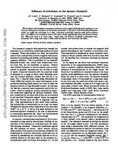
Fig. 2: (Colour on-line) Absolute equilibrium kinetic-energy spectrum and magnetic energy spectrum during the linear regime of dynamo growth (obtained with a small random initial magnetic seed) with k0 = 40 and Rm = 20 and resolution 1283 (corresponding to ζ = 0.86 in fig. 3(a)). Eu (k) still remains in absolute equilibrium as in the initial state, while Eb (k) has developed a tail and a dominant large-scale mode at k = 1. The dashed line in (a) represents the fit using eqs. (4) with α = 1.75 × 10⁶ and β = 4.15 × 10⁴ .
truncated Euler equation is known to reach at large times an absolute equilibrium that is a statistically stationary Gaussian exact solution of the associated Liouville equation [12]. When the flow has a non-vanishing helicity, the absolute equilibria of the kinetic energy and helicity were obtained by Kraichnan [13] and explicitly read
8π k4 β α2 1 − β 2 k 2 /α2 (4) with α and β determined by the initial kinetic energy and helicity. Note that if one intends to directly study the dynamo problem in the Pm → 0 limit, it amounts to setting ν = 0 Absolute equilibrium. – In the experimental context and f = 0 in eq. (1). In this limit, the velocity initial data of liquid metals, a more “realistic” computation would realone controls the flow on which the dynamo stability is quire to further decrease the magnetic Prandtl number. investigated. However, a huge resolution would then be needed to perAE dynamo with scale separation at Pm = 0 vs. form a DNS. Indeed, when Re is increased, modes with wave numbers beyond the scale separation range (kbox –k0 ) single-mode ABC dynamos at large Pm . – We now become populated by the turbulent cascade that takes turn to the study of the ABC kinematic dynamo problem place from forcing wave number k0 down to dissipative with zero forcing and zero viscosity. The initial ABC flow wave number kd ∼ k0 Re3/4 . is at k = k0 with small magnetic seed at k = kbox . As the Note that the turbulent dynamo problem is already a ABC flow is an exact but unstable solution of the Euler very difficult one, even without a scale separation range. equation, the roundoff error grows rapidly and the flow setIt was proposed to circumvent the difficulty of resolving tles into an absolute equilibrium as displayed in fig. 2(a). the large range of scales by combining direct numerical The steep rise of Eu (k) at high k is related to the denomsimulations with Lagrangian-averaged model and large- inator of eqs. (4). Dynamos are clearly present in helical absolute equilibria with growing large-scale magnetic field eddy simulations [2]. In the present work we propose to focus instead on the as shown in fig. 2(b). Figure 3(a) shows the computed growth rate of Eb for problem with a large scale separation and to make use of the special structure of the energy spectrum in the scale various Rm at resolution of 323 , 643 and 1283 with various separation range, that can be represented as a so-called values of ζ = k0 /kmax , where k0 is the wave number of the absolute equilibrium. Indeed, as noted above when dis- ABC initial data used to generate the absolute equilibrium cussing fig. 1(b), H(k)/E(k) vs. k 2 is almost linear up to of the Euler equation. (Beside scale separation, ζ also controls the helicity H = �u · ∇ × u � = 2k0 Eu .) k = 20 which is expected for AE (see eqs. (4) below). Figure 3(b) shows the critical Rm at which the inception Since the pioneering study of Lee (1952) [11] on the behavior of conservative systems with Fourier truncation of dynamo action takes place. The increase in ζ is seen at k = kmax , the dynamics of the unforced spectrally to result in a decrease in critical Rm . By inspection of Eu (k) =
29002-p3
4π k2 , α 1 − β 2 k 2 /α2
H(k) =
Srinivasa Gopalakrishnan Ganga Prasath et al. 40
a)
Critical Rm
Growth rate
0.5
0 ζ = 0.24
−0.5
ζ = 0.47 ζ = 0.71
b)
AE 128 Th 128 AE 64 Th 64 AE 32 Th 32
30 20 10
ζ = 0.86
−1 0
Rm
20
30
0.2
0.4
0.6 ζ
1
15
0 ζ = 0.24
−1
ζ = 0.47
10 Crit Rm(64)
5
Crit Rm(Th)
ζ = 0.71
−2 0
0.8
d)
c)
1 Critical Rm
Growth rate
2
10
Crit R (128) m
ζ = 0.86
10
Rm
20
Crit Rm(Th)
0 30
0
0.5
ζ
1
Fig. 3: (Colour on-line) Comparison of growth rates of magnetic energy Eb : (a) absolute equilibrium velocity field at resolution 1283 . (b) Critical Rm (determined by interpolation) together with theoretical scaling analysis at resolutions 323 , 643 and 1283 . (c) Same as (a) but for single-mode ABC flow. (d) Same as (b) but for single-mode ABC flow and resolutions 643 and 1283 .
the magnetic energy spectrum, the wave number kB of the growing dominant mode is found to be kbox = 1 (see fig. 2(b)). Note that maximal-helicity (ζ = 1) absolute equilibrium has critical Rm that is comparable with that of the forced ABC case (see table 1). Furthermore, 3D visualizations of the growing magnetic mode and the kinetic energy obtained for absolute equilibrium (fig. 4(a)) are very similar to those corresponding to the forced case (fig. 4(b)). It is apparent in fig. 2(a) that some of the AE kineticenergy spectra are rather well peaked at maximum wave number (as can be expected from eqs. (4)). This naturally leads us to study the problem of a single-mode ABC dynamo with scale separation. Note that the forcing will generate a single ABC mode at k = k0 in the limit Re → 0 or large Pm : the opposite limit to that studied with AE flows. The scale separation dependence of the single-mode large Pm number ABC kinematic dynamo is presented in fig. 3. Figure 3(c) shows the computed growth rate of Eb for various Rm at resolution of 1283 and at various values of ζ = k0 /kmax . Contrary to the case of the AE flow, the single-mode ABC initial condition displays an opposite bifurcation trend. An increase in ζ corresponds to an increase in critical Rm .
Fig. 4: (Colour on-line) Visualization of the growing magnetic field represented by arrows at a resolution of 1283 . (a) AE velocity, (b) forced ABC velocity. The 3D volume rendering corresponds to the kinetic energy of absolute equilibrium at maximum intensity. (k )
0 small scale u = u ABC , the magnetic field can be written � as b = B 0 + b , where B 0 is a large scale and b � a small scale. At first order in the small-scale magnetic Reynolds number b � = −(ηΔ)−1 ∇ × (u × B 0 ) and one finds that the average emf can be written as
αB 0 = �u × b � � = −
u2 B 0. ηk0
(5)
The resulting so-called α-effect evolution equation for B 0 is ∂t B 0 = α∇ × B 0 + ηΔB 0 (6) and implies criticality for ηc = |α|/kB , where kB is the wave number corresponding to B 0 . Thus, the critical Rm is given by � √ 2Eu k0 c = . (7) Rm = kB ηc kB
Note that this theoretical result is valid at first order in the small-scale Reynolds number in the limit of large scale Dependence of critical Rm on scale separation. – separation k0 /kB . With the moderate scale separation values used in the present work the scaling exponent of c Scaling of single-mode ABC dynamo. The scaling of Rm becomes apparent but the prefactor needs a correcthe critical Rm with scale separation k0 /kB can be under- tion. The large-scale computations, with resolution larger stood by the following argument. The growth of a large- than 10243, that are needed to check the convergence of scale magnetic field is governed by the electromotive force the prefactor to 1 are left for a future study. Figure 3(d) (emf) term u × b in the induction equation (2). With a shows the comparison of this scaling with the calculated 29002-p4
Dynamo action by turbulence in absolute equilibrium 2
�
k 2 H(k , ω) dk dω, ω2 + η2 k4
(8)
where H(k , ω) denotes the Fourier transform of the spatiotemporal helicity fluctuations. On dimensional √ grounds, the effective viscosity related to AE is given by Eu /k √ max and the velocity correlation time is given by kmax / Eu k 2 . Thus, the effective integration to values smaller √ √ range for ω in eq. (8) is limited than Eu k 2 /kmax . As ω/ηk 2 ∼ Eu /ηkmax � 1 at the dynamo threshold (in the limit of large scale separation) the integral over ω yields � H(k) 1 dk. (9) α∼ η k2 2 2
2
Equations (4) show that, for moderate values of β k /α , the absolute equilibrium helicity spectrum roughly scales as H(k) ∼ γk 4 and moreover the total helicity H = � kmax H(k)dk has a value H ≈ k0 Eu . This results in an 0 5 . approximate expression for γ given by γ ∼ 5k0 Eu /kmax Thus, the magnitude of α for absolute equilibrium veloc2 ity field is approximately given by αAE ∼ 5k0 Eu /3ηkmax . Similar to the case of ABC dynamo, the expression for the most unstable mode can be written as, kB = 2 η 2 which results in the expression for criti5k0 Eu /3kmax cal magnetic Rm given by � √ 2 2E 6kmax u c = ≈ . (10) Rm kB ηc 5kB k0
25
b)
20
R =10 m
1
−15
H(t)/2E(t)
−10
10
E (t) b
10
1.5
R =30
15
m
R =60 m
10
R =100
5
Rm=500
m
10 0.5
Scaling of the AE dynamo. Using first-order smoothing approximation, it has been shown [14] that η α=− 3
0
10
a)
−5
Eu(t)
critical Rm from numerical computations (at three different resolutions of 323 , 643 , 1283) with an additional factor of 2.25. The square-root behavior is clearly visible and is due to the α-effect where the scale separation is more discernible in the case of large k0 .
0
R =1000 m
0 50
100
150
t
200
250
−5 0
10
20
30
40
50
t
Fig. 5: (Colour on-line) (a) Evolution of kinetic and magnetic energy with time indicating saturation when k0 = 20 at resolution 643 . (b) Ratio of helicity to kinetic energy vs. time during the saturation and the decay of the magnetic field.
behavior of the dynamo generation due to both ABC flow and AE initial condition with maximum possible helicity at a given resolution. Figures 3(b) and (d) show that the critical Rm for both the scenarios are close to each other at high k0 where ABC flow and AE behave equivalently in generating a dynamo. Strikingly, in eqs. (7) and (10), the corresponding analytical expressions for critical Rm , have similar proportional behavior only when kmax = k0 with equivalent α-effect as well. Nonlinear saturation of the magnetic field for the AE dynamo. – The exponential growth of a magnetic field above the dynamo threshold first saturates because of the Lorentz-force back reaction on the flow. In a second stage, the magnetic field is observed to decay to zero exponentially in time (fig. 5(a)). This results from the absence of flow forcing (only a given initial amount of kinetic energy is present in the initial data). Although there is no viscous dissipation, the magnetic diffusivity alone is able to significantly dissipate the total energy (when the magnetic field has grown enough). Non-trivial effects are however found to take place in this framework. Both H and Eu decrease in time and saturate to constant values in the long time limit. Figure 5(b) shows that the long-time saturation value of H/Eu strongly depends on Rm . For small supercriticality (Rm ≤ 30) H/Eu is almost unchanged, whereas its saturation value decreases monotonously towards zero at larger Rm . The large Rm decrease of the saturation value is readily explained as follows. In the limit Rm → ∞ there is no dissipation and magnetic absolute equilibrium can take place. There are 3 invariants: total energy, magnetic helicity and cross-helicity, that completely define the magnetic equilibrium [15]. As the initial values of magnetic helicity and cross-helicity are very small, it is easy to show (see eq. (25) in reference [15]) that such equilibration will destroy the kinetic helicity. It is remarkable that the saturation value of the relative kinetic helicity H/Eu behaves monotonously with respect to the distance to the dynamo c (see fig. 5(b)). threshold Rm − Rm
Figure 3(b) shows the comparison of this scaling (with an additional prefactor of 2.25) with our AE numerical computations. It is visible that the trend persists up to a 1283 resolution. The beating mechanism explained above for ABC flow with a single mode acts on a wider scale for the AE spectrum since it possesses energy at varying length of the eddies. Thus, the interaction of high-energy small eddies in velocity results in the formation of tail-like feature in Eb (k) as seen in fig. 2(b). It is also the interaction of these small scales that results in the growth of a large-scale magnetic field. Now, in order to bring out the similarity between singlemode ABC and AE flow, we consider specific scenarios in Conclusion. – Using the results of our study we can both cases. From eqs. (4) it is visible that the spectrum becomes more pointed towards kmax for high initial helicity. conclude by proposing a new configuration for a future This spectrum is in some sense similar to the single-mode dynamo experiment. The idea is to drive a sodium flow ABC flow with k0 close to kmax . To wit, we compare the in a cubic meter of liquid sodium using a Roberts flow 29002-p5
Srinivasa Gopalakrishnan Ganga Prasath et al. forcing as in the Karlsruhe experiment but without constraining the flow in a periodic array of pipes. A Roberts flow forcing can be achieved using a square array of counterrotating vertical spindles, each of them fitted with several propellers. Both vertical and azimuthal flows are driven around each spindle, in a manner similar to a screw spindle pump. Both the vertical and azimuthal velocities change sign from one spindle to its neighbours. In contrast to the Karlsruhe experiment, a large-scale flow up to the size of the container, involving turbulent fluctuations, can develop in this device. From the hydrodynamic viewpoint, it will be of fundamental interest to characterize these hydrodynamic fluctuations and to check that their spectrum at wave numbers below the forcing scale do correspond to statistical equilibrium. To the best of our knowledge, the experimental study of turbulent spectra in this range has never been performed. The present study has shown that this type of flow involving both helical forcing and scale separation can provide an efficient way to reach a dynamo regime generated by a turbulent flow without geometrical constraints. This configuration can be an alternative to dynamo experiments using turbulent flows without scale separation [16–18] that have not displayed the dynamo effect so far, except when ferromagnetic impellers are used [19]. REFERENCES [1] Moffatt H. K., Magnetic Field Generation in Electrically Conducting Fluids (Cambridge University Press) 1978. [2] Ponty Y., Mininni P. D., Montgomery D. C., Pinton J.-F., Politano H. and Pouquet A., Phys. Rev. Lett., 94 (2005) 164502. [3] Gissinger C., Dormy E. and Fauve S., Phys. Rev. Lett., 101 (2008) 144502.
[4] Mininni P. D. and Montgomery D. C., Phys. Rev. E, 72 (2005) 056320. [5] Iskakov A. B., Schekochihin A. A., Cowley S. C., McWilliams J. C. and Proctor M. R. E., Phys. Rev. Lett., 98 (2007) 208501. [6] Mininni P. D., Phys. Rev. E, 76 (2007) 026316. [7] Frisch U., Fully developed turbulence and intermittency, in Proceedings of Turbulence and Predictability in Geophysical Fluid Dynamics and Climate Dynamics, edited by Gil M., Benzi R. and Parisi G. (Elsevier, Amsterdam; North-Holland) 1985, pp. 71–88. ¨ ller U., Phys. Fluids, 13 (2001) [8] Stieglitz R. and Mu 561. [9] Mininni P. D., Rosenberg D., Reddy R. and Pouquet A., Parallel Comput., 37 (2011) 316. [10] Gottlieb D. and Orszag S. A., Numerical Analysis of Spectral Methods (SIAM, Philadelphia) 1977. [11] Lee T., Q. Appl. Math., 10 (1952) 69. [12] Orszag S., J. Fluid Mech., 41 (1970). [13] Kraichnan R., J. Fluid Mech., 59 (1973) 745. [14] Moffatt H. and Proctor M., Geophys. Astrophys. Fluid Dyn., 21 (1982) 265. [15] Frisch U., Pouquet A., L´ eorat J. and Mazure A., J. Fluid Mech., 68 (1975) 769. [16] Peffley N. L., Cawthorne A. B. and Lathrop D. P., Phys. Rev. E, 61 (2000) 5287. [17] Spence E. J., Nornberg M. D., Jacobson C. M., Parada C. A., Taylor N. Z., Kendrick R. D. and Forest C. B., Phys. Rev. Lett., 98 (2007) 164503. [18] Colgate S. A., Beckley H., Si J., Martinic J., Westpfahl D., Slutz J., Westrom C., Klein B., Schendel P., Scharle C., McKinney T., Ginanni R., Bentley I., Mickey T., Ferrel R., Li H., Pariev V. and Finn J., Phys. Rev. Lett., 106 (2011) 175003. [19] Monchaux R., Berhanu M., Bourgoin M., Moulin M., Odier P., Pinton J.-F., Volk R., Fauve S., Mordant N., P´ etr´ elis F., Chiffaudel A., Daviaud F., Dubrulle B., Gasquet C., Mari´ e L. and Ravelet F., Phys. Rev. Lett., 98 (2007) 044502.
29002-p6