11, 13, 15 propose an approach di erent from the one ad- dressed above. ... Experimental results close the paper section 5 . 2 Basic de .... 1 g be the function which maps v 2 f0 1gp to the index j of the class K k j to which it ..... E2 = f010 011 111g. E1 is marked by .... Continued example: E1 is represented by the robdd bdd. 1.
Preprint from Proceedings of IFIP Workshop on Logic and Architecture Synthesis, pp.61-70, Grenoble, France, December 1994
E�cient ROBDD based computation of common decomposition functions of multi-output boolean functions Christoph Scholl
Paul Molitor
Department of Computer Science Universit�at des Saarlandes D 66041 Saarbr�ucken, FRG
Department of Computer Science Martin-Luther Universit�at Halle D-06099 Halle Saale�, FRG
Abstract
One of the crucial problems multi-level logic synthesis techniques for multi-output boolean functions f = �f1 � : : : � fm � : f0� 1gn ! f0� 1gm have to deal with is �nding sublogic which can be shared by di�erent outputs, i.e., �nding boolean functions � = ��1 � : : : � �h � : f0� 1gp ! f0� 1gh which can be used as common sublogic of good realizations of f1 � : : : � fm . In this paper we present an e�cient robdd based implementation of this Common Decomposition Functions Problem �cdf . The key concept of our method is the exploitation of equivalences of the functions f1 � : : : � fm which considerably reduces the running time of the tool. Formally, cdf is de�ned as follows: Given m boolean functions f1 � : : : � fm : f0� 1gn ! f0� 1g , and two natural numbers p and h, �nd h boolean functions �1� : : : � �h : f0� 1gp ! f0� 1g such that 81 � k � m there is a decomposition of fk of the form
fk �x1 � : : : � xn � = g�k� ��1�x1 � : : : � xp �� : : : � �h �x1 � : : : � xp �� ��hk+1� �x1 � : : : � xp�� : : : � ��rkk��x1 � : : : � xp �� xp+1 � : : : � xn � using a minimal number rk of single-output boolean decomposition functions.
1 Introduction
The long term goal for logic synthesis is the automatic transformation from a behavioral description of a boolean function to near-optimal netlists, whether the goal is minimum delay, minimum area, or some combination. Most of the approaches attacking the multi-level logic synthesis problem use gate count as optimization criterion. A survey can be found in 4 . Alternatively, some recent papers 10, 11, 13, 15 propose an approach di�erent from the one addressed above. This approach to multi-level logic synthesis which originates from Ashenhurst 1 , Curtis 8 , Hotz
9 , and Karp 12 is based on minimizing communication complexity. The methods used to reduce communication complexity employ functional decomposition, i.e., given a This work was supported in part by DFG grant SFB 124 and the Graduiertenkolleg of the Universit� at des Saarlandes
boolean function f : f0� 1gn ! f0� 1g they are looking for �multi-output� boolean functions �, � , and g, such that f �x1 � : : : � xn � = g���x1 � : : : � xp�� � �xp+1 � : : : � xn �� holds for all �x1 � : : : � xn � 2 f0� 1gn �see Figure 1�. If one
Figure 1: Decomposition 0� 1 n 0� 1
f g !f g
of a boolean function f :
wants to apply functional decomposition recursively to the decomposition functions � and � , a generalization to multi-output boolean functions is required. Of course, the approaches of the papers above can also be applied to multi-output boolean functions f = �f1 � : : : � fm� : f0� 1gn ! f0� 1gm either by considering multi-output boolean functions as single-output multi-value functions f 0 m: f0� 1gn ! f0� : : : � 2m � 1g de�ned by f 0 �x1 � : : : � xn � = i�1 i=1 fi �x1 � : : : � xn � � 2 or by decomposing each singleoutput boolean function fi independently of the other single-output functions fj �j 6= i� and only then testing whether they use some identical decomposition functions by chance. The �rst method has the drawback that it decomposes each single-output function fi with respect to the same input partition which can result in poor realizations. It does not take into consideration that there possibly exist single-output boolean functions fi and fj such that there does not exist one input partition good for both, fi and fj . Furthermore, even in case that there is an input partition good for every single-output function of f , it is unlikely
P
that there is a decomposition where function g has much less inputs than f �if m is large enough�, i.e., g is not much easier to synthesize than f . The drawback of the second method is clear. In the �nal analysis, it does not use the potential of reusing subcircuits for di�erent outputs of f . In �14� the authors presented a multi-level synthesis method for multi-output boolean functions based on communication complexity which avoids both drawbacks. The method can be divided into two steps. In the �rst step, output partitioning is performed, i.e., ff1 � : : : � fm g is partitioned into disjoint sets Y1 � : : : � Yu . Single-output functions fi and fj of the same set Yk will be decomposed with respect to the same input partition. The partitioning is executed such that for every Yk there is an input partition which is 'near-optimal' for every fi 2 Yk . In the second step, the decomposition functions of the singleoutput functions of each class Yk are constructed giving special attention to generate these functions in such a way that many of them can be used in the decomposition of di�erent elements of Yk . Benchmarking results of circuits taken from 1991 MCNC benchmark set have shown the technique to be e�ective with respect to layout size and signal delay. The paper in hand presents a much more e�cient version of our algorithms from �14�. During the computation of common decomposition functions we e�ciently make use of Reduced Ordered Binary Decision Diagrams �robdd�, which are compact representations for many of the boolean functions encountered in typical applications �6�. In this paper we show that it is possible to carry out all necessary steps based on robdd's. In particular we show that the computation of common decomposition functions for the decomposition of several single-output functions, which is the basis of step 2 of the technique above �14�, can be performed e�ciently based on robdd's. �The crucial point of this method is the exploitation of �equivalences� of the functions f1 � : : : � fm which results in the computation of connected components �in the graph-theoretical sense��. Benchmarking results show the new method to be e�cient with respect to layout size, signal delay and running time. We start by giving some basic de�nitions �section 2� and summarize the algorithm for computing common decomposition functions �section 3�. In section 4 we demonstrate how to apply robdds to implement this algorithm. Experimental results close the paper �section 5�.
2
Basic de�nitions A multi-output boolean function � with n inputs is represented as a set f�1 � : : : � �m g of boolean-valued output functions. We denote the set of completely de�ned boolean functions with n inputs and m outputs by Bn�m . Let Bn be an abbreviation for Bn�1 . �i�:::�j �i � j � denotes the tuple ��i � : : : � �j �.
De�nition 1 A decomposition of a multi-output boolean function f 2 Bn�m with respect to the input partition fX1 � X2 g �X1 = fx1 � : : : � xp g,X2 = fxp+1 � : : : � xp+q g, p+q = n� is a representation of f of the form
fk �x1 � : : : � xn � = g�k� ���1k� �X1 �� : : : � ��rkk��X1 �� �1�k� �X2�� : : : � �s�kk��X2 �� 0
0
�8k 2 f1� : : : � mg�, where ��ik� 2 Bp �8i�, �j�k� 2 Bq �8j �, and g�k� 2 Brk +sk . ��ik� and �j�k� are called decomposition functions of fk . g�k� is called composition function of fk .3 0
0
With respect to a given input partition fX1 � X2 g, a single-output function fk can be represented as a 2p � 2q matrix M �fk �, the decomposition matrix of fk or the chart of fk with respect to fX1 � X2 g. �For illustration see Figure 2.� Each row and column of M �fk � is associated with a distinct assignment of values to the inputs in X1 and X2 , respectively, such that fk �X1 � X2 � = M �fk ��X1 � X2 � where M �fk ��X1� X2 � represents the element of M �fk � which lies in the row associated with X1 and the column associated with X2 . Note that ���1k�� : : : � ��rk�� of de�nition 1 encodes the k rows of chart M �fk �. Of course, the following property has to hold. Encoding Property If the row pattern of row �v1 � : : : � vp � 2 f0� 1gp di�ers from the row pattern of row �v1 � : : : � vp � 2 f0� 1gp , then ���1k� � : : : � ��rkk� � has to assign di�erent codes to �v1 � : : : � vp � and �v1 � : : : � vp�. 3 The minimum number of communication wires required between the subcircuit which encodes the rows of M �fk � and the composition function g�k� is dlog p�1k� e where p�1k� is the number of distinct row patterns in M �fk �. rk will denote value dlog p1�k� e in the following. De�nition 2 A decomposition of fk : f0� 1gn ! f0� 1g is optimal �for X1 with respect to a given input partition A = fX1 � X2 g� if it uses only rk �= dlog p�1k� e� decomposition functions ��1k� � : : : � �r�kk� with domain X1 . 3 0
0
0
0
0
0
�
To compute decomposition functions �with domain X1 � of a multi-output function f which are used by di�erent single-output functions fk , we have to consider the following problem which will be denoted by cdf. �cdf can be posed for X2 in an analogous manner.� Given: Let f = ff1 � : : : � fm g2 Bn�m be a multi-output boolean function, A = fX1 � X2g with X1 = fx1 � : : : � xp g and X2 = fxp+1 � : : : � xn g be an input partition, and h be a natural number with h � rk �= dlog p�1k� e� �8k�. Find: h single-output boolean functions �1 � : : : � �h 2 Bp , which can be used as decomposition functions of every Likewise, the minimum number sk of interconnections between � �k� and g�k� is dlog p�2k�e where p�2k� is the number of distinct column patterns in M �fk �. �
f1
x4 00 x5 00
1 1
xn 01
1
x 1x 2x 3 0 0 0 0 1 1 1 1
0 0 1 1 0 0 1 1
0 1 0 1 0 1 0 1
f2
x 4 00 x 5 00
1 1
x n 01
1
��k� : f0� 1gp ! f1� : : : � p�1k� g be the function which maps v 2 f0� 1gp to the index j of the class Kj�k� to which it �
x 1x 2 x 3 row pattern 1 row pattern 1 row pattern 2 row pattern 2 row pattern 3 row pattern 3 row pattern 3 row pattern 2
0 0 0 0 1 1 1 1
0 0 1 1 0 0 1 1
0 1 0 1 0 1 0 1
belongs. Continued example: �see Figure 2� f0� 1g3 = 1 consists of 3 elements, namely K1�1� = f000� 001g, K2�1� = f010� 011� 111g, and K3�1� = f100� 101� 110g. It follows that ��1� �000� = ��1� �001� = 1, ��1� �010� = ��1� �011� = ��1� �111� = 2, and ��1� �100� = ��1� �101� = ��1� �110� = 3. f0� 1g3 = 2 consists of 4 classes, namely K1�2� = f000� 110g, K2�2� = f001� 100� 101g, K3�2� = f010g, and K4�2� = f011� 111g. 3 h Furthermore, for given �1�:::�h and all a 2 f0� 1g , let Sa�k� be the set f��k� �v�� �1�:::�h �v� = ag of those classes which contain a row mapped to a by �1�:::�h . ��1�:::�h is not able to tell these rows apart �see the Encoding Property�.� Note that Sa�k� and Sa�k� need not to be disjoint for a 6= a , and that the number j Sa�k� j of elements of Sa�k� equals the number of distinct row patterns of M �fk � mapped to a by �1�:::�h . Thus, maxfj Sa�k� j� a 2 f0� 1gh g denotes the 'inability to distinguish' of �1�:::�h with respect to fk . itd�A� fk � �1�:::�h � will denote value maxfj Sa�k� j� a 2 f0� 1gh g in the following. Continued example: Let h be equal 2. Assume that 8�v1 � v2� v3� 2 f0� 1g3 �1 �v1 � v2 � v3 � = v2 and �2 �v1 � v2 � v3 � = v3 . It follows that S00�1� = f1� 3g holds because �1�2 �000� = �1�2 �100� = 00 and ��1� �000� = 1, ��1� �100� = 3. Furthermore the following equalities hold: S01�1� = f1� 3g, S10�1� = f2� 3g, and S11�1� = f2g. Thus the inability to distinguish itd�A�f1 � �1�2 � of �1�2 with respect to f1 is equal to 2. 3
row pattern 1 row pattern 2 row pattern 3 row pattern 4 row pattern 2 row pattern 2 row pattern 1 row pattern 4
�
y
Figure 2: Charts M �f1 � and M �f2 � of the multi-output boolean function ff1 � f2 g which will be used to illustrate the ideas of the paper. The input partition A is given by �fx1 � x2 � x3 g� fx4 � : : : � xn g�. Each chart obviously consists of 8 rows. A row pattern is associated to each row. There are three �four� di�erent row patterns in M �f1 � �M �f2 �� denoted by the numbers 1, 2, and 3 �1 to 4�. Thus, r1 = r2 = 2 holds. single-output function fk for k = 1� : : : � m such that there is an optimal decomposition of fk of the form fk �x1 � : : : � xn � = g�k� ��1 �X1 �� : : : � �h �X1 �� ��hk+1� �X1 �� : : : � ��rkk� �X1 �� X2 �:
3
Of course, such h boolean functions need not to exist. We have proven the problem whether such functions �1 � : : : � �h exist to be NP-complete. Nevertheless, we have to solve cdf. An algorithm which is applicable from the practical point of view �as shown by the benchmarking results� is presented in the next two sections.
3 An algorithm for CDF
In the following, let f = ff1 � : : : � fm g2 Bn�m be a multioutput boolean function. Each single-output function fk has to be decomposed with respect to the same given input partition A = fX1 � X2 g �computed during output partitioning �see �14��� which will be �xed in the following.
3.1 Theoretical background
We start with a theoretical result working towards a solution to cdf. It gives a condition necessary and suf�cient that h single-output functions �1 � : : : � �h 2 Bp are common decomposition functions of f1 � : : : � fm. It is a generalization of a lemma shown by Karp �12�. For this, we need the following notations. The rows of chart M �fk � induce a partition of f0� 1gp into equivalence classes K1�k�� : : : � Kp�kk�� such that v� v 2 f0� 1gp belong to the 1 same class Kj�k� if and only if the two corresponding row patterns of M �fk � are identical. We denote the corresponding equivalence relation by �k and the set of the equivalence classes fK1�k�� : : : � Kp�kk�� g by f0� 1gp = k . Let 0
�
1
0
0
Lemma 1 �1 � : : : � �h 2 Bp are common decomposition
functions of f1 � : : : � fm with respect to A such that there is an optimal decomposition of fk of the form fk �x1 � : : : � xn � = g�k� ��1 �X1 �� : : : � �h �X1 �� ��hk+1� �X1 �� : : : � ��rkk��X1 �� X2 � �8k 2 f1� : : : � mg� if and only if the inability to distinguish itd�A� fk � �1�:::�h � of �1�:::�h with respect to fk is � 2rk h �8k�. 3 Proof: Since ��1�:::�h � ��hk+1� �:::�rk � has to assign di�erent values to rows of chart M �fk � with di�erent row patterns � �see the Encoding Property�, ��hk+1 �:::�rk has to assign different values �to those rows which cannot be told apart by �1�:::�h . As �hk+1� �:::�rk can produce at most 2rk h di�erent values, the statement of the lemma follows. �
�
3.2 The basic algorithm
cdf can be solved by computing �1�:::�h by a �simpli�ed� branch and bound algorithm. The sets Sa�k� , which determine the inability to distinguish itd�A� fk � �1�:::�h � with respect to fk , are constructed step by step. In the initialization phase, �1�:::�h �v � is set to undef for all v 2 f0� 1gp , 0
y
0
Remember that 1�:::�h denotes the tuple � 1 � : : : � h �.
and Sak� is set to the empty set for all a and k. Each time we enter the main loop �step 4 of the algorithm� see Figure 3� there is a v 2 f0� 1gp and a vector a 2 f0� 1gh such that �1�:::�h �v � is de ned for all v with int�v � � int�v�, and there is no extension of the present function table with �1�:::�h �v� = a and int�a � � int�a� which does not violate the condition of lemma 1. In this step we test whether the condition of lemma 1 is violated if �1�:::�h �v� is set to a. If the condition is violated, we have to backtrack if int�a� = 2h � 1, i.e., a = �1� : : : � 1�. If int�a� � 2h � 1, we enter the loop once again with a incremented by 1. The sets Sak� are updated in each step. �Thus, the numbers itd�A� fk � �1�:::�h � of lemma 1 are implicitely updated, too.� For detailed information of the algorithm see the pseudo code shown in Figure 3. Continued example: Assume h = 1, and remember that r1 = r2 = 2 holds. The cdf algorithm above computes �1 : f0� 1g3 ! f0� 1g de ned by �1 �v� = 1 �� v 2 f010� 011� 111g as common decomposition function of f1 and f2 . The inability to distinguish with respect to fk �k = 1� 2� is equal to 2 as S01� = f1� 3g, S11� = f2g, and S02� = f1� 2g, S12� = f3� 4g: 3 0
0
0
0
0
0
z
0
x
1. Let Sak� = � �81 � k � m� a 2 f0� 1gh �, �1�:::�h �v � = undef �8v 2f0� 1gp �, v = �0� : : : � 0� 2f0� 1gp , and a = �0� : : : � 0� 2f0� 1gh . 2. Let �1�:::�h �v� = a, =* �1�:::�h �0� : : : � 0� = �0� : : : � 0� *= Sak� = f� k� �v�g �8k�. 3. Increment v. 4. Let �1�:::�h �v� = a. If �8k� j Sak� f� k� �v�gj� 2r h =* test whether the condition of lemma 1 is not violated *= then let Sak� = Sak� f� k� �v�g �8k�. Increment v. Let a = �0� : : : � 0� 2f0� 1gh . else while �1�:::�h �v� == �1� : : : � 1� do let �1�:::�h �v� = undef . Decrement v� "S�k1� v� = S�k1� v� n f� k� �v�g" 8k. 0
4.1 Some observations
The rst observation, already made in �7, 13�, is that for all �v1 � : : : � vp � 2 f0� 1gp the row pattern belonging to row �v1 � : : : � vp � of M �fk � equals the function table of the cofactor �fk �x11 ::: x �with x0i = xi and x1i = xi �. Thus the problem of determining the number p1k� of di�erent row patterns of M �fk � is equivalent to the problem of computing the number of di�erent cofactors �fk �x11 ::: x . The robdd of the cofactor �fk �x11 ::: x is given by the sub-bdd of bddk whose root is reached by starting at the root of bddk and then following the path corresponding to �v1 � : : : � vp �. The roots of these cofactors are called linking nodes �the shaded nodes in Figure 4�. Since fk is given by a robdd, the number of di�erent linking nodes of bddk obviously equals the number of di�erent cofactors. The computational complexity of determining the number of di�erent linking nodes is at most linear in the size of bddk since it can be determined by traversing bddk in a depth
rst search manner. v
�
vp
� p
v
v
�
�
vp
� p
vp � p
int y� denotes the natural number represented by the boolean vector y Because of itd A�fk � �1 � = 2, there obviously exists a decomposition function �2k� : f0� 1g3 ! f0� 1g such that 8v�v 2 f0� 1g3 �1 v���2k� v�� 6= �1 v ���2k� v �� if the row patterns of chart M fk � coresponding to v and v are di erent k = 1� 2�. z
x
0
0
0
0
0
k�
�:::�h
od
�:::�h
a = �1�:::�h �v�. Increment a. Let �1�:::�h �v� = undef .
4 A ROBDD based implementation
Assume the function f = ff1 � : : : � fm g 2 Bn�m we want to decompose is given by m robdds bdd1 � : : : � bddm and that the ordering of the variables is given by �x1 � : : : � xn � �for illustration see Figure 4�. Then, the following observations result in an e�cient implementation.
0
0
� 5. If �8v 2f0� 1gp � �1�:::�h �v� 6= undef then return �1 � : : : � �h . else if v = �0� : : : � 0� then return "There is no solution" else goto 4 � � Figure 3: Pseudo code of the algorithm solving cdf. In
step 2 of the algorithm, we can set �1�:::�h �0� : : : � 0� = �0� : : : � 0� without loss of generality because if there exist h common decomposition functions then there also exist h common decomposition functions with �1�:::�h �0� : : : � 0� = �0� : : : � 0�. Furthermore, the operation S�k1� v� = S�k1� v� n f� k� �v�g in step 4 is somewhat more complex than common set di�erence: the index � k� �v� is only removed from S�k1� v� if there is no v 6= v with int�v � � int�v�, �1�:::�h �v � = �1�:::�h �v�, and � k� �v � = � k� �v�. �:::�h
�:::�h
0
0
�:::�h
0
0
The second observation is that encoding the linking nodes of bddk with a code of length rk �which is the logarithm of the number of linking nodes of bddk � results in an optimal decomposition of fk . �Of course this simple approach does not lead to common decomposition functions.� For 1 � i � rk the corresponding decomposition function �ik� is given by substituting the linking nodes of bddk by the ith bits of the codewords belonging to the linking nodes. The composition function g k� is given by
corresponding row patterns in M �f1 � or M �f2 � are identical, i.e., if v �1 v or v �2 v . �Edges resulting from f1 are drawn in bold.� This results in a graph whose connected components determine the equivalence classes Ei . There are two classes, namely E1 = f000� 001� 100� 101� 110g and E2 = f010� 011� 111g. E1 is marked by shaded nodes. 3 0
bdd 1
bdd 2 x1
x1 x2
x2
x2
x2 x3
x3
x3
x33
x4
x5
x4
x5
x4
x4
x4
1
3
2
1
2
3
4
0
000 111
001
The robdds of f1 and f2 . The left �right� outgoing edge of node xi corresponds to the case xi = 0 �xi = 1�.
Figure 4: Continued example:
substituting the part of bddk , which corresponds to the variables x1 � : : : � xp , by the corresponding code-tree. For illustration see Figure 5. A decomposition constructed in this way leads to decomposition functions ��jk� of fk which assign the same value to all those �v1 � : : : � vp � 2 f0� 1gp for which the corresponding row patterns of M �fk � are identical. �Note that till now the decomposition functions ��1k� � : : : � ��rkk� of a single-output function fk are allowed to assign di�erent values to rows with identical row patterns in the case that the total number of di�erent row patterns is less than 2rk .� In order to use this simple method of constructing the decomposition functions and composition functions, the branch and bound algorithm above is modi ed so that only equivalence preserving decomposition functions are considered. We will name the modi ed algorithm �robdd based branch and bound algorithm�. De�nition 3 A decomposition function �i 2 Bp of a boolean function fk 2 Bn is said to preserve equivalences if �i �v� = �i �v0 � holds for every v� v0 2f0� 1gp with v �k v0 .3
Thus, common equivalence preserving decomposition functions �1 � : : : � �h of f1 � : : : � fm have to assign the same value to v and v 2 f0� 1gp whenever there is a k 2 f1� : : : � mg such that the rows of M �fk � corresponding to v and v have identical row patterns. More formally, let 0
0
def �91 � k � m� v �k v � v � v �� 0
0
then the corresponding equivalence relation partitions the rows, i.e. f0� 1gp , into equivalence classes E1 � : : : � El such that common equivalence preserving decomposition functions have to assign the same value to each v 2 Ei . We will denote the set of these equivalence classes by f0� 1gp = . Continued example: Figure 6 illustrates the de nition of this equivalence relation. Consider a graph whose vertices are the 8 rows 000� : : : � 111. �Note that this graph will not be constructed by the algorithm presented in subsection 4.2.2.� There is an edge between two rows v and v if the �
0
010
110
101
011 100
Figure 6: Continued example:
Illustration of the de nition of the equivalence classes Ei . Thus, the robdd based branch and bound algorithm assigns values to the subsets E1 � : : : � El . Because l mostly is much smaller than 2p , this approach considerably reduces the running time compared to the original branch and bound algorithm �see subsection 3.2�. �The benchmarking results will also show that this reduction of the running time can be achieved without reducing the quality of the circuits constructed.� During the robdd based branch and bound algorithm, every time a value a 2f0� 1gh is assigned to an equivalence class Ei by �1�:::�h , the sets Sa�k� �8k�, which contain the di�erent row patterns of M �fk � mapped to a by �1�:::�h , have to be updated by Sa�k� = Sa�k� SETi�k� . SETi�k� denotes the set fj � Kj�k� Ei g, i.e., the set which consists of the indices �with respect to ��k� � of the di�erent row patterns of M �fk � belonging to Ei . Note that the sets SETi�k� and SETj�k� are disjoint if i 6= j . Continued example: SET1�1� = f1� 3g, SET2�1� = f2g, SET1�2� = f1� 2g, and SET2�2� = f3� 4g. 3 Of course, the robdd based branch and bound algorithm requires a preprocessing and postprocessing phase described in the following. 4.2 Preprocessing steps In the rst preprocessing step we have to e�ciently determine the minimum number rk of decomposition functions required for a decomposition of fk �8k�. In the second preprocessing step we construct robdds representing the equivalence classes Kj�k� 2 f0� 1gp = k . Then, we determine the robdds of the equivalence classes f0� 1gp = corresponding to ff1 � : : : � fm g and thus also the corresponding sets SETi�k� the algorithm requires. �
�
α(12)
x2
x2 x3
0
α(2) 2
x1
x3
0
x3
1
0
y1 x2
x2 x3
1
g(2) x1
x3
1
y2
y2 x3
x3
0
1
x5
x4
x4
x4
1
2
3
4
Figure 5: Continued example:
Optimal decomposition of f2 by encoding the �rst linking node by 00, the second by 01, the third by 10 and the fourth by 11. �To make things clear the obdds shown are not reduced.� Note that all these computation steps have to be done without constructing the charts M �fk �. Since we have already explained in section 4.1 how to e�ciently determine the minimum number rk of decomposition functions required for a decomposition of a function fk , it remains to show how to e�ciently compute the equivalence classes.
4.2.1 Computation of the equivalence classes with respect to k As already mentioned, identical row patterns of M �fk � correspond to the same linking node of bddk . Thus every equivalence class Kj�k� is associated to exactly one linking node n�jk� and vice versa. Kj�k� is given by the set of the paths from the root of bddk to linking node n�jk� . Thus, substituting the sub-bdd of bddk with root n�jk� by constant 1 and connecting every edge which leaves the cone of n�jk� to constant 0 results in a robdd, whose ON-set is given by �k � �k � �k � Kj . We call this robdd bddj . The cone of node nj is de�ned to be the set of those nodes x of bddk such that there is a path from x to n�jk� . For illustration see Figure 7.
4.2.2 Computation of the equivalence classes with respect to � We implicitely construct a graph G = �V� E � where the set of vertices is given by the robdds bdd�jk� representing the equivalence classes Kj�k�. At the end, there is an undirected edge fbdd�jk11 � � bdd�jk22 � g if and only if bdd�jk11 � ^ bdd�jk22 � 6= �, i.e., i� their ON-sets are not disjoint �see Figure 8�. Obviously, there is a one-to-one relation between the set of the connected components �in the graph-theoretical sense� of G and the set of the equivalence classes f0� 1gp = . For every class Ei , there is a connected component C Ci of G such that the logical-or of the robdds bdd�jk� �for any �xed k � corresponding to vertices of C Ci results in a representation of Ei and vice versa. V
Continued example: E1 is represented by the robdd �1� �2� �2� _ bdd�1� 3 which is the same robdd as bdd1 _ bdd2 . �1� E2 is represented by bdd2 which is the same robdd as �2� bdd3 _ bdd�2� . 3 4 bdd1
bdd
(2) 1
(1) 1
bdd
(2)
bdd2 (1) 2
bdd
(2) 3
bdd (1) 3
bdd
(2) 4
bdd
Figure 8: Continued example: Computation of the equivalence classes f0� 1gp = . The connected components of
graph G represent the classes Ei .
Note that the algorithm described below does not have to test each pair of robdds bdd�jk11 � , bdd�jk22 � whether their ON-sets are disjoint. Virtually, it performs depth �rst search on graph G. In each step we compute a connected component which contains a node bdd�1� not yet touched z by calling procedure search�bdd�1� z � 1�. This procedure recursively constructs robdds cc�1�� : : : � cc�m�. At each moment cc�k� equals the robdd representing the logical-or of all the nodes bdd�jk� of the present connected component which have already been touched. At the end of procedure call search�bdd�1� z � 1�, the equation cc�1� = : : : = cc�m� holds, and cc�1� represents the connected component computed. The exact implementation of search is shown in Figure 9. Note that, if the robdd notcovered is non-
(1)
bdd (1) 3
bdd (1) 2
bdd 1
x1
x1
x1 x2
x2
x2
x2 x3
1
OBDDs
(1) bdd j specifying
(2)
bdd 2
x1 x2
x3 1
0
x1 x2
x2
x2
x3
0
0
bdd 4 x1
x2
x2 x33
x3
0
(2)
bdd 3
x1 x2
1
the rows with identical row patterns in M(f1 )
(2)
(2)
bdd 1
1
1
0
0
x3
x33
x3
1
0
1
(2)
OBDDs bdd j specifying the rows with identical row patterns in M(f2 )
Figure 7: Continued example: Illustration the obdds shown still have to be reduced.� procedure
search
�bdd
b,
int
of how to e�ciently compute the equivalence classes f0 1gp = k . �Note that
k�
b as touched� cc � = cc � _ b =* logical-or of two robdds *= for j = 1 to m do if j 6= k then notcovered = b ^ cc � =* logical-and *= while notcovered 6= � do let v be element of ON �notcovered�. � let bdd be the robdd � with v 2 ON �bdd �. � call search�bdd j � notcovered = b ^ cc � =* logical-and *= mark k
k
j
j u
j u
j u
j
od� fi�
od�
Figure 9: Pseudo code of the algorithm computing the equivalence classes f0 1gp =�
empty during a step, there is a row v belonging to the present connected component which is not in the ON-set of cc j� yet, so that the robdd bdduj� which describes the set of the rows which have identical row patterns as v in M �fj � has to be joined to cc j� . Procedure search is called exactly once for every node of G. During the execution of the body of procedure search�b k� �without the recursive calls� there are one ap-
ply operation �see 2, 6�� performing the logical-or of two robdds and at most m � 1 + degree�b� apply operations performing logical-and of two robdds, where degree�b� denotes the degree of vertex b with respect to G. This results in a number of apply operations which is linear in the size of G as m � 1 � degree�b� holds. The running time of the remaining operations is linear in the size of the relevant robdd. 4.3 Postprocessing steps After the execution of the preprocessing steps, the robdd based branch and bound algorithm encodes the equivalence classes as already described.
4.3.1 Computation of the ROBDDs of the decomposition functions
Assume that a single-output function �i has been found by the robdd based algorithm which can be used as decomposition function of fk . Note that the algorithm does not explicitly assign values to every v 2 f0 1gp but only to the equivalence classes f0 1gp =� . As the robdd of these equivalence classes are known, we only have to connect by logical-or those robdds whose corresponding equivalence classes are mapped to value 1 by �i in order to obtain the robdd representing �i . Continued example: Assume h = 1. The robdd based branch and bound algorithm constructs �1 : f0 1g3 ! f0 1g de�ned by �1 �E1 � = 0 and �1 �E2 � = 1 as common decomposition function of f1 and f2 . Thus the robdd of �1 is 2�given by the robdd specifying E2 , and equals function �1 of Figure 5. 3
4.3.2 Computation of the ROBDDs of the composition functions Once that rk boolean valued functions �1k� � : : : � �rkk� which can be used to decompose function fk are determined, we have to compute the robdd of the corresponding composition function g k� . This is done as �informally� described in section 4.1 �second observation�. For illustration see Figure 5 once again. The robdd of g k� can be constructed using the linking nodes njk� and combining these cofactors through the codetree with if-then-else-operations of the robdd-package 2 .
5 Benchmarking results
We have synthesized several examples of the 1991 MCNC multi-level logic benchmark set in order to compare factor, factorII 10, 11 , which are communication based multi-level synthesis tools developed at PennState University, and misII 5 , sis 1.1 16 to our tool which uses the cdf algorithm described above as basis. We will call the robdd based implementation of our tool mulopII. The former implementation working on charts will be called mulop. As running time considerations motivate this paper, we compared the running times of our robdd based implementation mulopII to those of our former version mulop. Table 1 shows gate countsy and running times for some of the MCNC multi-level logic benchmark circuits. The running times are measured on a SPARCstation 10�30 �64 MByte RAM�. The experiments show that the robdd based implementation is much faster than the former version. For these examples mulop has running times up to about 50 CPU minutes while the running time of mulopII is at most a few seconds. In particular, these experiments prove our synthesis tool to be applicable in terms of running time. Although the running times of mulopII are much smaller than those of our former version mulop, in almost all cases the numbers of gates of the computed circuits are not larger. We compared mulopII to factor, factorII. We ran the experiments with the technology mapping used in 11 . Since the quality of the layouts synthesized by factorII approximately equals the quality of the layouts synthesized by factor �see 11 �, Table 2 only reports the results of the comparison of mulopII and factorII. �The results concerning factorII are those which are published in 11 .� Compared to factorII, our approach generates realizations with a smaller �or equal� number of gates for almost all circuits. As layout considerations motivate the approach of minimizing communication complexity, we compared layout sizes in the following. A comparison to factorII with respect to layout size was not possible because factorII and The �maximal� value of parameter h of cdf is determined by logarithmic search. More details of how the cdf algorithm is integrated in the tool can be found in �14�. y The library consists of the 2-input gates from stdcell2 2.genlib available in octtools.
Number of No. of gates Circuit inputs outputs factorII mulopII ratio 9symm1 9 1 75 52 1.44 cm138a 6 8 21 21 1.00 cm151a 12 2 37 40 0.93 14 5 80 41 1.95 cm162a cm163a 16 5 47 36 1.31 5 3 18 14 1.29 cm82a cmb 16 4 33 34 0.97 decod 5 16 31 32 0.97 8 8 107 54 1.98 f51m x2 10 7 65 51 1.27 z4m1 7 4 25 21 1.19 Table 2: Comparison between our tool mulopII and factorII with respect to the number of gates used. The technology �le used is taken from the paper of Hwang et al. Note that it is di�erent from the technology �le in the other comparisons. the layout tool used in the paper of Hwang et al. was not at our disposal. We used the standard cell place and route package wolfe which is integrated in octtools. Table 3 shows the comparison between mulopII, misII and sis 1.1 with respect to layout size. The technology library used consists of the set of the 2-input gates.z For almost two thirds of the benchmark set, our approach dominates �or is as good as� that of misII and sis with respect to layout size. The signal delays of our realizations for more than two thirds of the circuits considered are better �or equal� than those of the realizations synthesized by misII and sis. However, on the other hand the results con�rm the observation already made in �10, 11� that some circuits, e.g., cm151a, are not suited for being decomposed with respect to disjoint input partitions. The most dramatic improvement has been obtained for circuit 9symm1 which is a symmetric function. This con�rms the approach of searching equivalence preserving decomposition functions. x
6
Conclusion
We have presented a robdd based technique of computing common decomposition functions of multi-output boolean functions. This algorithm has been integrated in our multi-level synthesis tool which has been presented in �14� where more details of how the cdf algorithm is integrated can be found. The benchmarking results show that most of the circuits constructed by our synthesis tool are very e�cient. They also prove it to be applicable in terms of running time. z For the technology le itself see available 22 in octtools. x Let : f0 1gm ! f0 1gn be a boolean function which is symmetric in some variables. Then, each equivalence preserving decompositionfunction of is symmetricin these variables, too. stdcell
f
�
�
f
:genlib
No. of gates Running time Circuit mulop mulopII ratio mulop mulopII ratio 9symm1 40 45 0.89 1.40 sec 1.23 sec 1.14 C17 6 7 0.86 0.32 sec 0.15 sec 2.13 cm138a 20 18 1.11 1.01 sec 0.18 sec 5.61 cm151a 48 41 1.17 4.16 sec 1.09 sec 3.82 cm152a 34 27 1.26 2.15 sec 0.50 sec 4.30 cm162a 46 44 1.05 350.65 sec 3.32 sec 105.62 cm163a 38 34 1.12 2923.31 sec 2.35 sec 1243.96 cm82a 13 13 1.00 0.38 sec 0.21 sec 1.81 cm85a 42 42 1.00 7.46 sec 3.73 sec 2.00 cmb 24 29 0.83 1836.13 sec 2.52 sec 728.62 decod 31 28 1.11 26.15 sec 2.56 sec 10.21 f51m 64 56 1.14 3.14 sec 1.83 sec 1.71 majority 9 9 1.00 0.44 sec 0.08 sec 5.50 parity 15 15 1.00 111.06 sec 1.37 sec 81.07 z4m1 20 20 1.00 0.66 sec 0.76 sec 0.87 Table 1: Comparison between the �prototype� robdd based implementation of our synthesis tool mulopII and the former version mulop working on decomposition charts. The technology �le consists of the 2-input gates from stdcell2 2.genlib available in octtools.
Layout size ratio Signal delay ratio misII sis mulopII misII sis misII sis mulopII misII sis 917928 1194336 201400 4.56 5.93 26.0 27.6 13.6 1.91 2.03 28800 28800 31744 0.91 0.91 4.2 4.2 4.2 1.00 1.00 101528 103896 87480 1.16 1.19 5.8 5.8 6.8 0.85 0.85 102528 95312 177712 0.58 0.54 12.6 12.6 16.4 0.77 0.77 90360 85536 106704 0.85 0.80 10.0 10.0 13.2 0.76 0.76 149736 131976 192000 0.78 0.69 13.8 12.0 13.2 1.05 0.91 153272 144008 164416 0.93 0.88 11.0 13.0 10.4 1.06 1.25 83104 74784 61600 1.35 1.21 8.2 7.2 7.0 1.17 1.03 171584 165456 180000 0.95 0.92 10.2 10.2 11.0 0.93 0.93 198616 204792 123496 1.61 1.66 14.8 9.4 6.8 2.18 1.38 133496 140448 119496 1.12 1.18 6.2 6.2 5.0 1.24 1.24 536016 561184 251392 2.13 2.23 51.0 51.0 18.4 2.77 2.77 42200 42200 39168 1.08 1.00 7.8 7.8 6.6 1.18 1.18 96976 99408 96976 1.00 1.03 6.2 5.0 5.0 1.24 1.00 176160 156288 103896 1.70 1.50 18.0 16.2 9.8 1.74 1.65 2982K 3228K 1937K 1.54 1.67 205.8 198.2 147.4 1.40 1.34 Table 3: Comparison between mulopII, misII, and sis1.1 with respect to layout size, and signal delay. Circuit 9symm1 C17 cm138a cm151a cm152a cm162a cm163a cm82a cm85a cmb decod f51m majority parity z4m1
P
References
1� R.L. Ashenhurst. The decomposition of switching functions. In Proceedings on an International Symposium on the Theory of Switching held at Comp. Lab. of Harvard University, pages 74�116, 1959. 2� K. Brace, R. Rudell, and R. Bryant. E cient implementation of a BDD package. In IEEE�ACM Design Automation Conference DAC90, pages 40�45, 1990. 3� R.K. Brayton, C.T. McMullen G.D. Hachtel, and A.L. Sangiovanni-Vincentelli. Logic Minimization Algorithms for VLSI Synthesis. The Kluwer International Series in Engineering and Computer Science. Kluwer Academic Publishers, 1984. 4� R.K. Brayton, G.D. Hachtel, and A. L. SangiovanniVincentelli. Multilevel logic synthesis. Proceedings of the IEEE, 78�2�:264�300, February 1990. 5� R.K. Brayton, R. Rudell, A. L. SangiovanniVincentelli, and A.R. Wang. MIS: A multiple-level logic optimization system. IEEE Trans. on CAD, CAD-6�11�, November 1987. 6� R.E. Bryant. Graph-based algorithms for boolean function manipulation. IEEE Trans. on Computers, C-35�8�:677�691, August 1986. 7� S. Chang and M. Marek-Sadowska. BDD representation of incompletely speci�ed functions. In Notes of the International Workshop on Logic Synthesis held in Tahoe City, California, May 1993. 8� H.A. Curtis. A generalized tree circuit. J. Assoc. Comput. Mach., 8:484�496, 1961. 9� G. Hotz. Zur Reduktionstheorie der booleschen Algebra. In Colloquium �uber Schaltkreis- und SchaltwerkTheorie, 1960. 10� T. Hwang, R.M. Owens, and M.J. Irwin. Exploiting communicaton complexity for multilevel logic synthesis. IEEE Trans. on CAD, CAD-9�10�:1017�1027, October 1990. 11� T. Hwang, R.M. Owens, and M.J. Irwin. E cient computing communication complexity for multilevel logic synthesis. IEEE Trans. on CAD, CAD11�5�:545�554, May 1992. 12� R.M. Karp. Functional decomposition and switching circuit design. Journal of Society of Industrial Applied Mathematics, 11�2�:291�335, June 1963. 13� Y. Lai, M. Pedram, and S. Vrudhula. BDD based decomposition of logic functions with application to FPGA synthesis. In IEEE�ACM Design Automation Conference DAC93, pages 642�647, 1993. 14� P. Molitor, C. Scholl. Communication based multilevel synthesis for multioutput boolean functions. In Proceedings of the 4th Great Lakes Symposium on VLSI, Notre Dame, Indiana, March 1994.
15� U. Schlichtmann. Boolean Matching and Disjoint Decomposition for FPGA Technology Mapping. In Proceedings of the IFIP Workshop on Logic and Architecture Synthesis, pages 83�102, 1993. 16� E. Sentovich et al. SIS: a system for sequential circuit synthesis. Department of EE and CS, UC Berkeley, May 1992.