e-mail classification using deep networks - Journal of Theoretical and ...

Journal of Theoretical and Applied Information Technology st

31 March 2012. Vol. 37 No.2 © 2005 - 2012 JATIT & LLS. All rights reserved.

ISSN: 1992-8645

www.jatit.org

E-ISSN: 1817-3195

E-MAIL CLASSIFICATION USING DEEP NETWORKS 1

1

AHMAD A. AL SALLAB, 2MOHSEN A. RASHWAN Department of Electronics and Communications Engineering

2

Prof., Department of Electronics and Communications Engineering E-mail: [email protected], [email protected]

ABSTRACT Email has become an essential communication tool in modern life, creating the need to manage the huge information generated. Email classification is a desirable feature in an email client to manage the email messages and categorize them into semantic groups. Statistical artificial intelligence and machine learning is a typical approach to solve such problem, driven by the success of such methods in other areas of knowledge management. Many classification methods exist, of which some have been already applied to email classification task, like Naïve Bayes Classifiers and SVM. Deep architectures of pattern classifiers represent a wide category of classifiers. Recently, Deep Belief Networks have demonstrated good performance in literature, driven by the fast learning algorithm using Restricted Boltzmann Machine model by Hinton et al, and the improvement in computing power which enables learning deep neural networks in reasonable time. Many datasets and corpus exist for email classification, with the most famous one is Enron dataset, made public by FERC, annotated and processed by many entities like SRI and MIT. In this paper, a machine learning approach using Deep Belief Networks is applied to email classification task, using the Enron dataset to train and test the proposed model. Keywords: Deep Belief Networks (DBN), Restricted Boltzmann Machine (RBM), Knowledge Management, Email Classification, Enron Email Dataset

1.

INTRODUCTION

With the huge amount of digital information in our life, Knowledge Management (KM) of such information has become essential. For example, to google a topic, the search engine needs to apply some sort of information retrieval based on the subject of the topic. Machine learning has been the choice for such KM tasks. Email usage has become an essential component of everyday life. With the increasing dependency on emails as a communication tool, the size of information generated also increases, which creates a real need to manage such huge amount of data. The most widely spread tool of email management are spam classifiers, which is a common ingredient in nearly all email clients. Spam classification is a two class pattern recognition problem. Naïve Bayes has been a success in that area giving fairly good results [1]. Average number of received emails per day varies between ten to hundreds and could be thousands for some categories of people. Subjects of daily emails

are sparse. For someone in business, categories of emails vary from business, family, fun, ads…etc. Even within each category, many sub-categories also exist. A normal behavior is to cluster those emails into semantic groups, and decide their importance to process them. Modern email clients may perform important/not important categorization based on some key words. Again this is a two class machine learning problem. Some more advanced clients could extract relevant information of the email, like appointments and meetings, based on date and time keywords. To save time and effort, a generic classification tool is needed to categorize emails in whatever categories the used desire. This is now a multi-class machine learning problem. To approach the solution of such problem, many classifiers exist, like SVM, ANN, and Naïve Bayes…etc. In all the aforementioned approaches, a features vector representing the email should be developed to model the emails. A common form of features vector is the bag-of-words, where a vocabulary of the most common words encountered in the emails is gathered to build the dimension of the vector length. Then each word is marked in this vector to

241

Journal of Theoretical and Applied Information Technology st

31 March 2012. Vol. 37 No.2 © 2005 - 2012 JATIT & LLS. All rights reserved.

ISSN: 1992-8645

www.jatit.org

E-ISSN: 1817-3195

exist or not in any given email. Another variant of such binary marking is the word count model, in which the word frequency is stored in the features vector.

then concluded with the main results, contributions and future works.

Following to composing the features vector, a training phase is required to train the model using statistical methods. After the model is trained, testing or evaluation phase should start, on completely different and independently formed set of examples.

Email classification into Spam/Non-spam has been a rich area of research for many years. Example of previous works on anti-spam filters can be found in [1][2] and [3].

For email classification task in particular, the corpus or dataset that is used for testing and training form a bottleneck. Two options exist, either build own dataset or use some publicly available corpus. Locally designed datasets require a huge manual effort for annotation and processing. On the other hand, there is no much publicly available sets, due to privacy and legitimacy issues for the private nature of email messages. Following the bankruptcy of Enron Corp., the Federal Energy Regulatory Commission (FERC) has made their email corpus public for research after their investigations. SRI, MIT and other entities have made efforts to process and annotate the dataset. Many variants exist, like with/without attachments, irrelevant categories removed…etc. Recent work by Hinton et al [6][11] and [12] on learning deep ANN architectures using Deep Belief Networks (DBN) model has showed good results, specially on high dimensional data, and document retrieval tasks [12]. The algorithm makes use of high dimensional data for pre-training, which is a nice feature for an email classifier that can be used for adaptation based on actual emails when the tool is in operation. In this paper, DBN Classifier is proposed as a solution for the multi-class email classification problem, in addition to a proposed approach to adapt the classifier in an unsupervised fashion based on real world emails. In the following sections, previous works are demonstrated, followed by review of the DBN classifier and its fast learning algorithm. The next section presents the pre-processing details of the Enron dataset to prepare it for usage with the DBN classifier. The proposed DBN classifier is then presented, with the details of pre-training and classification. Finally, the system evaluation results are presented. Results of the new approach are compared to previous works on Enron datasets in literature. The paper is

2.

PREVIOUS WORK ON EMAIL CLASSIFICATION

Email categorization into generic multi-classes has been studied in literature using SVM, Maximum Entropy, Winnow, K-NN and Naïve Bayes classifiers. The datasets used are usually variants of Enron dataset. Some other research in literature has been done on locally made datasets, other than Enron. Work in [6] suggests a co-training algorithm using SVN and Naïve Bayes, done on local dataset, with 2-class classification problem. The experiment done in [6] is simplified in terms of number of classes (only 2) and dataset size (only 1500 total training and test sets size). Results show maximum accuracy of 83% on Naïve Bayes and 87% on SVM. Work in [7] tries TF-IDF method also on local dataset. Research in [4] marks the start of using Enron as a corpus of e-mail classification tasks. In addition to presenting the Enron dataset itself, SVM classifier performance on Enron dataset is also presented in [4]. Bekkerman et al [5] have worked on email classification on Enron dataset for the SVM, Naïve Bayes, Winnow and Maximum Entropy classifiers. In [9] K-NN classifier was tested on E-mail categorization using Enron dataset, introducing a new algorithm called the Gaussian balanced K-NN. 3.

REVIEW OF DEEP BELIEF NETWORKS CLASSIFICATION

Artificial Neural Networks (ANN) have been used for decades for classification tasks. It has grabbed the attention of researchers due to the similarity between its architecture and the human brains. The ANN is formed of several stacked D layers, each of width

N i neurons. The weights relating each W(i )(i 1)

consecutive layer i and i+1 is

242

matrix of

Journal of Theoretical and Applied Information Technology st

31 March 2012. Vol. 37 No.2 © 2005 - 2012 JATIT & LLS. All rights reserved.

ISSN: 1992-8645

www.jatit.org

N i  N i 1 . The width of input layer is N denoted by 0 and the last layer by M.

dimension

The main focus of research in ANN is on training the network, i.e. to find the right weights that can be used to correctly classify the input examples. The most successful algorithm in that area is the famous back propagation algorithm. The problem with back propagation is the following; ANN represents a non-linear mapping f(X,W), where X is the input vector and W is the weight matrix of the whole network, as the number of layers increases, the function f gets more complicated, such that it contains multiple local minima. The back propagation algorithm converges to a certain minimum based on the initialization of weights W. Sometimes it gets stuck to a poor performance local minimum and not the global one. For some AI tasks, those local minima are fine, but not accepted for other cases. Also, back propagation training time is not scalable with the depth of the network. As the number of layers increases, training time gets much higher. This could not be a big problem with the increasing power of computer nowadays.

E-ISSN: 1817-3195

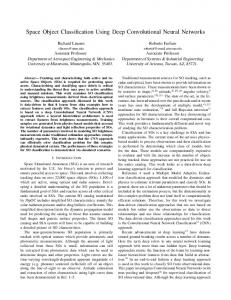
3.1. DEEP BELIEF NETWORK MODEL The algorithm is based on modifying the ANN model from discriminative to generative model. The discriminative model is the one which models the classification performance of the network. The objective function to be minimized is the error between the required classification targets and the obtained ones. On the other hand, the generative model is the one that models the generation of original data capability of the network. The objective is to minimize the error between the model-generated data and the original one. The generative model must be able to re-generate the original data given the hidden units states, this represents its belief of the real world data. This kind of model is called Deep Belief Network (DBN). The DBN model enables the network to generate visible activations based on its hidden units’ states, this represents the network belief. The problem now is how to get the hidden units states corresponding to the visible data. A Restricted Boltzmann Machine is proposed between each two consecutive layers of the network. The difference between ANN, DBN and RBM is shown in Figure 2.

Another disadvantage of back propagation is that it requires high supply of labeled data, which could not be available for many AI tasks requiring classification. For the aforementioned problems, Hinton et al. have introduced a fast learning algorithm based on Deep Belief Networks (DBN) and Restricted Boltzmann Machine (RBM) to train a deep ANN

Figure 2 (a) ANN (b) DBN (c) RBM 3.2. PRE-TRAINING PHASE To optimize a given configuration of visible and hidden units, the model energy is to be minimized.

E ( v , h )    v j h j w ij

N D 1  M

i, j

w  w  w

ND2

w   N1

E (v , h )  v j h j  learning _ signal  w ij

N0

Our objective for a generative model is to maximize the probability of visible units’ activations p(v). To get p(v) we have to marginalize the p(v,h) probability for the whole configuration. Figure 1 Deep Artificial Neural Network

243

Journal of Theoretical and Applied Information Technology st

31 March 2012. Vol. 37 No.2 © 2005 - 2012 JATIT & LLS. All rights reserved.

ISSN: 1992-8645

p ( v, h ) 

www.jatit.org

e  E (v,h )  allpossibleconfigurations

e  E ( v ,h )  e  E (v,h )

and Organizes). It contains data from about 150 users, mostly senior management of Enron, organized into folders. This data was originally made public, and posted to the web, by the Federal Energy Regulatory Commission during its investigation. The email dataset was later purchased MIT, and turned out to have a number of integrity problems. The dataset was further processed by SRI [2] [14].

v ,h 

e

 E (v,h )

 partitionfunction  PF

v ,h 

e  p (v )   p ( v , h )  e

E-ISSN: 1817-3195

 E (v,h )

h

 E ( v ,h )

h

v ,h 

For mathematical convenience, let’s maximize the log p(v) instead of p(v) itself. Moreover, to maximize the data generation with respect to model belief, we adjust the weights such that model belief is decremented while the real data is incremented as follows:

w(

logp(v) logp(v) Realdata  Model) wij wij

( vihj Realdata  vihj Model) Finally the pre-training algorithm is simply to apply the data on the input layer of the 2-layer RBM to get the hidden activations, and then re-generate the model visible activations, and finally generate the model hidden activations. In this way the RBM weights can be updated for the given input data. Having the current layer trained, its weights are frozen, and the hidden layer activations are used as the next layer visible inputs, and the same training algorithm is applied. The obtained Deep network weights are used to initialize a fine tuning phase.

Figure 3 shows the directory structure of the dataset. Each user has a folder, which contains folder by category, which could further split into sub-folder representing sub-categories. Some of these folders are irrelevant for classification task, like “sent”, “inbox”, “deleted”…etc… Preprocessing is needed to extract useful categories. Also, preprocessing is needed to extract useful vocabulary, build features vectors…etc. Training and test sets are built by randomly splitting the processed dataset into training and testing examples. This random splitting guarantees independence between test and training sets. More information about the processed dataset will be discussed in 6.1.

Enron Email Directory

arnold-j

3.3. FINE-TUNING PHASE

shapiro-r

inbox

computers

tax

Figure 3 Enron email directory structure

The fine tuning phase is simply the ordinary back propagation algorithm. For classification tasks, a layer of width equals the number of targets or classes, is added on top of the network. Each neuron of this layer is activated for each class label while the others are deactivated. The back propagation starts from the weights obtained in pretraining phase. The top layer activations are obtained for each training set example, or batch of examples, is obtained in the forward path, and then the error signal between the obtained activations and required targets is back propagated in the network for weights adjustment. 4.

beck-s

The dataset is organized as shown in Figure 3. Each user represents a sub-directory. Each sub-directory contains another level of sub-directories representing the categories of received messages. Further division of categories into sub-categories is possible for some cases. The message structure is composed of two parts; the first one is the message header, containing some data of the message information, like the To/From/CC/BCC fields, the date, the subject, attachments…etc. The second part is the mail body itself in text format.

ENRON DATASET PREPROCESSING

Enron dataset was collected and prepared by the CALO Project (A Cognitive Assistant that Learns 244

Journal of Theoretical and Applied Information Technology st

31 March 2012. Vol. 37 No.2 © 2005 - 2012 JATIT & LLS. All rights reserved.

ISSN: 1992-8645

www.jatit.org

Message-ID: Date: Tue, 17 Apr 2001 12:39:10 -0700 (PDT) From: [email protected] To: [email protected] Subject: RE: EEX bid Mime-Version: 1.0 Content-Type: text/plain; charset=us-ascii Content-Transfer-Encoding: 7bit X-From: Gottlob, Edward X-To: Farmer, Daren J. X-cc: X-bcc: X-Origin: FARMER-D X-FileName: darren farmer 6-26-02.pst

Jill is not representing the pipeline anymore Brian Riley should be handling this for EEX

E-ISSN: 1817-3195

To build this vocabulary vector, the whole corpus of each user is parsed, and the words are ordered discerningly in terms of the frequency they are encountered in the dataset, and then the most L frequently encountered words are selected as the members of V . The parameter L is chosen based on experimental results, where L is chosen to give the best accuracy.

Message header information

During vocabulary building, irrelevant words are ignored (“he”, “she”, “when”…etc). Also, e-mail header is excluded, which contains the actual class label. Message body

4.3. CATEGORIES BUILDING Categories of e-mail messages are simply the different class targets of the classification problem at hand. Each user has own set of categories as discussed in 4.1. Number of categories is denoted by N _ t arg ets , which is the dimension of class

Figure 4 Email format in Enron dataset

(i )

of the ith example.

4.1. USERS SELECTION

labels y

E-mails of the Enron employees are really diverse, so that not limited number of common categories can be easily identified among all users. For example for a user, the corpus is divided into: “eol”, “ces”, “entex”, “industial”…etc. While for another user his mails are categorized into: “duke”, “ecogas”, “bastos”…etc. This creates a difficulty assigning labels to each e-mail based on its category, since categories are different between users.

Selection of categories per each user directory is done first by counting the number of e-mails in each category. This counting is done recursively, i.e. if the category contains sub-categories, then messages in the sub-folders are also counted. Then the categories are ordered discerningly, and the highest score ones are selected as the targets labels N _ t arg ets .

To overcome this problem, users are ordered discerningly in terms of the number of e-mails in their directories, and then the top users with largest number of e-mails were selected as the input datasets, so that, each user directory represents a separate dataset. This ensures coherency between each category e-mail examples.

Each target of N _ t arg ets is assigned a binary code of N _ t arg ets bits, with only one bit set to 1 and the others set to 0. Each category is assigned an integer number from 0 to N _ t arg ets  1 which is denoted by label. The target label y

(i )

of the ith e-mail is a binary

4.2. VOCABULARY BUILDING

vector of length N _ t arg ets , with only 1 set at

E-mail classification is based on categorizing a

2 label position. N _ t arg ets is chosen based on

(i )

th

features vector x of the i example into one of N _ t arg ets categories. The features themselves are just indicators of the existence of certain, mostencountered words in the dataset, called the vocabulary of the corpus, or the bag-of-words. The (i )

size L of x is the number of vocabulary words. Since, each user is considered a separate dataset, hence, each user is assigned a separate vocabulary vector V .

experimental results so as to give the best accuracy. During the aforementioned process, the irrelevant categories are dropped, since they have no relevance to the classification problem, like “inbox”, “sent”, “deleted”…etc. 4.4. FEATURES EXTRACTION (i )

The features vector representing the ith e-mail x could be one of two cases; either binary or word-

245

Journal of Theoretical and Applied Information Technology st

31 March 2012. Vol. 37 No.2 © 2005 - 2012 JATIT & LLS. All rights reserved.

ISSN: 1992-8645

www.jatit.org

count. For both cases, the vocabulary of the bag-ofwords V is considered, and vector.

x

(i )

is an L size

For the binary case, the features vector N _ t arg ets is just a vector of 1’s or 0’s. The 1 indicates the existence of the corresponding vocabulary word in the e-mail, while 0 marks its absence. For the wordcount case, values in x (i ) are integers, marking the frequency of word repetition within the given email. In the proposed classifier, binary features were tested to give the good results, while wordcounts give poor results, and hence binary features shall be considered.

PROPOSED DBN CLASSIFIER

The e-mail classifier proposed is based on Deep Neural Network, trained using the algorithm described in 3. The Enron dataset is used as the email corpus used in both training and testing, split in the way described in 4. Features are extracted in the same way described in 4.4. The algorithm is composed of two stages; the first one is training a stack of RBM’s with the unlabeled training set examples, and the second phase is to fine tune a deep ANN using back propagation, starting from the weights obtained in pre-training. The next sections describe the two stages in details. 5.1. RBM TRAINING

4.5. TRAINING AND TEST SETS SELECTION For each user, the features and labels are extracted as described in the above sections. Now, to split the processed dataset into training and testing sets, a complete random approach was followed, such that training and testing e-mails were selected randomly from the final dataset. This ensures independence between training and testing datasets.

(x(0) , y(1) )   (1) (1)  ( , ) x y   .    .   .    ( N1) ( N1) (x  ,y ) 

5.

E-ISSN: 1817-3195

 ( X 0 ( 0 ) )   (1)  ( X 0 )   .    .   1) (N ( X 0 batch )   Batch ( i )    ( X 1( 0 ) )   (1) ( X )   1  .    .  ( N batch 1)  ( X )  Batch ( i )  1  

 ( X D2( 0) )   (1)  ( X D2 )  .    .  ( Nbatch 1)  ( X D 2 )   Batch(i ) 

In the pre-training phase, the model is composed of several layers of RBM’s; each takes the form of Figure 2(c).

  ( X 1( 0 ) )   (1)  ( X 1 )  .    .  ( N batch 1)  ( X1 )   Batch ( i ) 

[W ] N 0  N1

[W ] N1  N 2

[W]ND2ND1

Figure 5 Pre-training dataflow graph 246

 ( X 2 ( 0 ) )   (1) ( X )   2  .    .  ( N batch 1)  ( X )  Batch ( i )  2  

 ( X D1( 0) )   (1)  ( X D1 )  .    .  ( Nbatch 1)  ( X D1 )   Batch(i ) 

Journal of Theoretical and Applied Information Technology st

31 March 2012. Vol. 37 No.2 © 2005 - 2012 JATIT & LLS. All rights reserved.

ISSN: 1992-8645

www.jatit.org

Figure 5 shows the general dataflow graph of the training algorithm. The dataset is first sub-divided into N batches, each of size N batch . The pretraining is completely unsupervised, so the dataset vectors labels must be removed. The labeled dataset

, y ( i ) ) , where x (i ) is the feature (i ) vector of example i, while y is the example’s (i ) label. Each x has size of L features, determined members are ( x

(i )

E-ISSN: 1817-3195

The activations of the visible layers are denoted by v while those of hidden layer are denoted by h . The activations of the hidden layer are used as visible data of the next layer data (i  1) . 5.2. ANN BACK PROPAGATION After the network is pre-trained as RBM-Stack model, the weights are further adjusted using back propagation.

for each user in the way described in 4.4, while (i )

each y has size of the number of categories or targets determined for each user as described in 4.3. The unlabeled examples [ X

(i )

] matrices of size

N batch are then fed to the first RBM of the stack as being the visible data. The RBM is trained by adjusting the weights so as to maximize the original data weight and reduce the model believed data weight as described in 3.2. Once an RBM of a given layer is trained, the weights of that layer are fixed, and the hidden activations of such layer are used as visible data of the next one. The algorithm continues till all layers are trained.

Fine tuning stage is fully supervised, i.e. the categories labels adjustment.

y (i ) are kept for weight

The whole dataset is divided into N , each of size N batch . The examples of each batch are denoted by X

(i )

. The corresponding class targets (i )

are denoted by Y . Those examples are fed into a Feed-forward ANN to obtain the classifier decision. The error signal between the classifier decision and (i )

is then back-propagated in the required target Y the network to adjust the weights. The whole process is repeated on all batches.

Training of each RBM is run in batch mode, i.e. weights are adjusted for each batch of examples. Sub_ routine_ pre_ train_ RBM(unlabeled_ dataset) data(1) : unlabeled_ dataset for i : 1 : N _ layers

(x(0) , y(1) )   (1) (1)  (x , y )  .    .  .    (x(N1) , y(N1) )

 ( X ( 0 ) , Y ( 0 ) )   (1) (1)  ( X , Y )  .    .  ( N Batch 1) ( N Batch 1)  ,Y ) ( X Batch ( i )

for j : 1 : N v( j)  data(i) h( j)  W T Ni Ni 1 .v( j) WNi Ni 1   (v( j)  h( j) WNi Ni 1  WNi Ni 1  WNi Ni 1 data(i  1)  h( j) end_for end _ for

Figure 7 Back propagation fine tuning

return(W ) Figure 6 RBM pre-training algorithm

Figure 6 describes the RBM pre-training algorithm. The number of layers of the network is denoted by N _ layers . The weights linking layers i and i+1

W are denoted by N i  N i1 . Each layer is fully trained using all N batches, before the next layer is trained. 247

Journal of Theoretical and Applied Information Technology st

31 March 2012. Vol. 37 No.2 © 2005 - 2012 JATIT & LLS. All rights reserved.

ISSN: 1992-8645

www.jatit.org

E-ISSN: 1817-3195

Sub _ routine _ fine _ tuning() W (1)  Sub _ routine _ pre _ train _ RBM () for i : 1 : N

6.1. PROCESSED DATASETS

class_t arg ets  Feed _ forward ( X (i ) , W (i)) 1 E (i)  (class_t arg ets  Y (i ) ) 2 2 W (i)  back _ propagation( E (i), W ) W (i)  W (i)  W (i) end _ for return (W )

Enron dataset pre-processing described in 4 results in different dataset for each user. The different parameters are: o Training set size o Testing set size o Number of categories/Class labels o Number of features Table 1 shows the details of each user’s dataset after pre-processing described in 4. User

Training set size (e-mails)

arnold-j baugmann beck-s blair-l cash-m griffith-j haedickem hayslett-r kaminski-v kean-s ruscitti-k shackletons shapiro-r steffes-j ward-k farmer-d kitchen-l lokay-m sanders-r williamsw3 campbell-l

90 952 891 1123 216 352 60

Figure 8 Fine tuning algorithm 5.3. CLASSIFICATION Now, all ANN layers weights are adjusted to achieve the minimum training error. To perform classification of a new (test) example, the features are first extracted as in 4.4, then the obtained vector is applied to the ANN. The classifier decision is obtained by feeding the feature vector forward into the ANN using the obtained W weights during training phases as in Figure 9.

E-mail

Features extraction

as text

Feed forward ANN [W]

E-mail Category

` Figure 9 Classification of a new e-mail 6.

SYSTEM EVALUATION

As described in 4.5, each user dataset is split randomly into training and testing sets, independent of each other. To evaluate the system, the ANN trained on the training set is tested on the test set, i.e. each of the e-mails in the test set is applied to the ANN classifier, and the classifier decision, obtained in 5.3, is compared to the actual class label, to obtain the classification error.

Err _ user 

 Misclassified _ mails

Total _ mails _ per _ user Accuracy _ user  (1  Err _ user )%

%

256 1791 1146 92 490 490 503 283 2589 1992 2073 711 1974 14

Test set size (emails) 10 106 100 15 23 64 31 658 55 231 79 168 118 95 95 665 864 61 281 26 14

Number of categori es 10 5 10 16 6 8 2 4 10 4 3 4 5 7 8 11 10 6 6 5 6

Number of features 100 1000 2000 1000 1000 1000 1000 2000 1000 10000 1000 1000 10000 1000 1000 1000 1000 1000 1000 1000 1000

Table 1 Users datasets details The total number of test set e-mails is 3,759 messages, while the total training set e-mails are 18,262 messages. The average number of features is around 1900 features, representing the vocabulary words. While the average number of mails categories is around 6 categories.

248

Journal of Theoretical and Applied Information Technology st

31 March 2012. Vol. 37 No.2 © 2005 - 2012 JATIT & LLS. All rights reserved.

ISSN: 1992-8645

www.jatit.org

6.2. NETWORK ARCHITECTURE The ANN architecture used for classification is 4layers architecture. The first layer has 500 neurons, the second has 500 neurons and the third layer has

E-ISSN: 1817-3195

2000 neurons. This architecture is common to all users. At the top layer, a variable width layer is added, with the number of neurons equal to the number of categories resulting from pre-processing step described in 4.3.

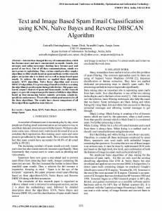
Figure 10 Network architecture 100% on many datasets: haedicke-m, ruscitti-k and shackelton-s.

6.3. RESULTS PER USER Figure 11 shows the accuracy of classification for each user dataset. Average accuracy is 87.24% overall datasets. Minimum accuracy is 51.57% on kitchen-l dataset. While Maximum accuracy is

Figure 11 Accuracy (%) results per user

249

Journal of Theoretical and Applied Information Technology st

31 March 2012. Vol. 37 No.2 © 2005 - 2012 JATIT & LLS. All rights reserved.

ISSN: 1992-8645

www.jatit.org

6.4. COMPARISON WITH OTHER CLASSIFIERS LITERATURE

E-ISSN: 1817-3195

compare to. In [9] a new algorithm, Gaussian Balanced K-NN is introduced.

IN

E-mail Classification task has been tested in many previous works as described in 2. However, only few of them, [4], [5] and [9], were found relevant to compare to, since they were conducted on Enron dataset as done in this paper.

Our results presented in Table 1 are averaged for all users to get average accuracy. The best classifier in literature is the SVM, which scores 71.53% accuracy. For the proposed DBN, the average score is improved to 87.24%.

In [4] SVM classifier was tested and averaged on all users. In [5] classifiers tested include: Naïve Bayes, SVM, Winnow and Maximum Entropy classifiers. Results are conducted per user. To be able to compare, results were averaged for all tested users. This work represents a good benchmark to

Also, in [5] and [9] results are provided per user. Experiments were conducted on the same users using the proposed DBN classifier. Results shown in Table 3 indicate the improvement of DBN classification accuracy over the classifiers tested in [5].

Table 2 Comparison with other works in [5] and [9] on Enron dataset

Average Accuracy

DBN

SVM [4]

SVM [5]

87.24%

70%

71.53%

Naïve Bayes [5] 57.5%

Maximum Entropy [5] 70.8%

Winnow [5]

K-NN [9]

68.4%

63.86%

Table 3 Comparison of classification accuracy (%) [5] and [9] on user basis DBN

beck-s farmer-d kaminski_v kitchen-l lokay-m sanders-r williamsw3

7.

SVM [5]

85.0

56.4

Naïve Bayes [5] 32.0

49.9

48.87

79.86

77.5

64.8

76.6

74.6

66.52

82.11

57.4

46.1

55.7

51.6

53.58

51.57

59.1

35.6

58.4

54.6

48.31

80.87

82.7

75.0

83.6

81.8

72.58

88.57

73.0

56.8

71.6

72.1

77.27

97.54

94.6

92.2

94.4

94.5

78.53

CONCLUSION

In this paper, a Deep ANN classifier is proposed for e-mail classification task. The training algorithm used is based on DBN and RBM training algorithm by Hinton et al. Enron e-mail corpus was used, since it is the most widely used and rich dataset in literature. A lot of pre-processing was done to prepare the dataset for classification task. First a reduced set is extracted to form smaller datasets, with the users of highest number of messages in their folders. Each user dataset is considered a separate task.

Maximum Entropy [5] 55.8

Winnow [5]

K-NN [9]

words. Also, e-mail categories are identified per user as the ones including the highest number of messages, excluding the irrelevant ones. Once the vocabulary and categories are built, the features can be extracted for each e-mail example. Training and testing sets are formed randomly from the given e-mail corpus. The DBN classifier is pre-trained using RBM model then fine-tuned using back propagation. The resulting network is used directly for classification. The used architecture is 500-500-2000 plus a top layer of number of neurons equal the number of target categories of classification.

Then, the vocabulary is built for each user for the most encountered words, excluding irrelevant 250

Journal of Theoretical and Applied Information Technology st

31 March 2012. Vol. 37 No.2 © 2005 - 2012 JATIT & LLS. All rights reserved.

ISSN: 1992-8645

www.jatit.org

Results per user are presented. Accuracies vary from 51.57% to 100% depending on the user. System evaluation is done based on comparison with previous works on e-mail classification using Enron database, to unify the base of classification to be on the same dataset. Comparison results reported indicate noticed improvement in the classification accuracy than the best reported results. The SVM classifier is reported to give average accuracy of about 71%, while DBN classifier gives 87.03% of average classification accuracy. Future work include testing some classifiers, known to give good results, like SVM, using the same dataset splitting and features, to have unified common base of comparison. Also, word-count features could results be tested and enhanced. REFERENCES : [1] Ion

[2]

[3]

[4]

[5]

[6]

Androutsopoulos, John Koutsias, Konstantinos V. Chandrinos, Constantine D. Spyropoulos T.S. Bhatti, R.C. Bansal, and D.P. Kothari, “An experimental comparison of naive Bayesian and keyword-based anti-spam filtering with personal e-mail messages”, SIGIR '00 Proceedings of the 23rd annual international ACM SIGIR conference on Research and development in information retrieval, 2000 Karl-Michael Schneider, “A comparison of event models for Naive Bayes anti-spam e-mail filtering”, EACL '03 Proceedings of the tenth conference on European chapter of the Association for Computational Linguistics, 2003 V. Cheng, C. H. Li, “Personalized Spam Filtering with Semi-supervised Classifier Ensemble”, Proceeding WI '06 Proceedings of the 2006 IEEE/WIC/ACM International Conference on Web Intelligence Bryan Klimt and Yiming Yang, “The Enron Corpus: A New Dataset for Email Classication Research”, Language Technologies Institute, Carnegie Mellon University, CEAS conference, 2004. Ron Bekkerman, Andrew Mccallum, G. Huang, “Automatic Categorization of Email into Folders: Benchmark Experiments on Enron and SRI Corpora”, Citeseer, vol 418, p 1-23 , 2004 S. Kiritchenko, S. Matwin “Email classi_cation with co-training” In Proc. of the 2001Conference of the Centre for Advanced

E-ISSN: 1817-3195

Studies on Collaborative Research, page 8, Toronto, Ontario, Canada, 2001. [7] R. B. Segal and J. O. Kephart. MailCat “An Intelligent Assistant for Organizing E-Mail”. In Proc. of the 3rd International Conference on Autonomous Agents, 1999. [8] W.A. Awad , S.M. ELseuofi “Machine learning methods for E-mail classification”, International Journal of Computer Applications (0975 – 8887), Volume 16– No.1, February 2011 [9] Pablo Bermejo, Jose A. Gamez, Jose M. Puerta, Roberto Uribe “Improving KNN-based e-mail classification into folders generating classbalanced datasets”, Proceedings of IPMU'08, pp. 529-536,June 22-27, 2008 [10] G. E. Hinton, S. Osindero, and Y. Teh, ‘‘A fast learning algorithm for deep belief nets’’ Neural Computation , vol. 18, pp. 1527---1554, 2006. [11] G. E. Hinton, ‘‘To Recognize Shapes, First Learn to Generate Images’’ Computational Neuroscience: Theoretical Insights into Brain Function, Elsevier, UTML TR 2006 --- 004, October 26, 2006 [12] Ruslan Salakhutdinov, ‘‘Learning Deep Generative Models’’ PhD thesis, Graduate Department of Computer Science, University of Toronto, 2009 [13] A. Sallab, M. Rashwan “Self Learning Machines using Deep Networks”, in Proceedings of 2011 International Conference of Soft Computing and Pattern Recognition (SoCPaR), pp. 21 – 26, 14-16 Oct. 2011 [14] http://www.cs.cmu.edu/~enron/, 1/11/2012

251