Mar 15, 2018 - Reed et al., 2014]. Our margin ... operator s : si=yk max{0,γ ..... [Boyd and Vandenberghe, 2004] Boyd, S. and Vandenberghe, L. (2004). Convex.
arXiv:1803.05598v1 [stat.ML] 15 Mar 2018
Large Margin Deep Networks for Classification Gamaleldin F. Elsayed∗
Dilip Krishnan
Hossein Mobahi
Kevin Regan
Samy Bengio
Google Research {gamaleldin,dilipkay,hmobahi,kevinregan,bengio}@google.com
Abstract We present a formulation of deep learning that aims at producing a large margin classifier. The notion of margin, minimum distance to a decision boundary, has served as the foundation of several theoretically profound and empirically successful results for both classification and regression tasks. However, most large margin algorithms are applicable only to shallow models with a preset feature representation; and conventional margin methods for neural networks only enforce margin at the output layer. Such methods are therefore not well suited for deep networks. In this work, we propose a novel loss function to impose a margin on any chosen set of layers of a deep network (including input and hidden layers). Our formulation allows choosing any lp norm (p ≥ 1) on the metric measuring the margin. We demonstrate that the decision boundary obtained by our loss has nice properties compared to standard classification loss functions. Specifically, we show improved empirical results on the MNIST, CIFAR-10 and ImageNet datasets on multiple tasks: generalization from small training sets, corrupted labels, and robustness against adversarial perturbations. The resulting loss is general and complementary to existing data augmentation (such as random/adversarial input transform) and regularization techniques (such as weight decay, dropout, and batch norm).
1
Introduction
The large margin principle has played a key role in the course of machine learning history, producing remarkable theoretical and empirical results for classification [Vapnik, 1995] and regression problems [Drucker et al., 1997]. However, exact large margin algorithms are only suitable for shallow models. In fact, for deep models, computation of the margin itself becomes intractable. This is in contrast to classic setups such as kernel SVMs, where the margin has a nice analytical form (the l2 norm of the parameters). Desirable benefits of large margin classifiers ∗ Work
done as a member of the Google AI Residency program g.co/airesidency.
1
(a)
(b)
cross entropy: test accuracy 98%
large margin: test accuracy 99%
Figure 1: Illustration of large margin. (a) The distance of each training point to the decision boundary, with the shortest one being marked as γ. While the closest point to the decision boundary does not need to be unique, the value of shortest distance (i.e. γ itself) is unique. (b) Toy example illustrating a good and a bad decision boundary obtained by optimizing a 4-layer deep network with cross-entropy loss (left), and with our proposed large margin loss (right). The two losses were trained for 10000 steps on data shown in bold dots (train accuracy is 100% for both losses). Accuracy on test data (light dots) is reported at the top of each figure. Note how the decision boundary is better shaped in the region outlined by the yellow squares. This figure is best seen in PDF. include better generalization properties and robustness to input perturbations [Cortes and Vapnik, 1995, Bousquet and Elisseeff, 2002]. To overcome the limitations of classical margin approaches, we design a novel loss function based on a first-order approximation of the margin. This loss function is applicable to any network architecture (e.g., arbitrary depth, activation function, use of convolutions), and complements existing generalpurpose regularization techniques such as weight-decay and dropout. We illustrate the basic idea of a large margin classifier within a toy setup in Figure 1. For demonstration purposes, consider a binary classification task and assume there is a model that can perfectly separate the data. Suppose the models are parameterized by vector w, where each model g(x; w) maps the input vector x to a real number, as shown in Figure 1(a); where the yellow region corresponds to positive values of g(x; w) and the blue region to negative values; the red and blue dots represent training points from the two classes. Such g is sometimes called a discriminant function. For a fixed w, g(x; w) partitions the input space into two sets of regions, depending on whether g(x; w) is positive or negative at those points. We refer to the boundary of these sets as the decision boundary, which can be characterized by {x | g(x; w) = 0} when g is a continuous function. For a fixed w, consider the distance of each training point to the decision boundary. We call the smallest such distance the margin. A large margin classifier seeks model parameters w that attain the largest margin. Figure 1(b) shows the decision boundaries attained by our new loss (right), and another solution attained by the standard cross-entropy loss (left). The yellow squares show regions where the large margin solution better captures the correct data distribution.
2
Margin may be defined based on the values of g (i.e. the output space) or on the input space. Despite similar naming, the two are very different. Margin based on output space values is the conventional definition. In fact, output margin can be computed exactly even for deep networks [Sun et al., 2015]. In contrast, the margin in the input space is computationally intractable for deep models. Despite that, the input margin is often of more practical interest. For example, a large margin in the input space implies immunity to input perturbations. Specifically, if a classifier attains margin of γ, i.e. the decision boundary is at least γ away from all the training points, then any perturbation of the input that is smaller than γ will not be able to flip the predicted label. More formally, a model with a margin of γ is robust to perturbations x + δ where sign(g(x)) = sign(g(x + δ)), when kδk< γ. It has been shown that standard deep learning methods lack such robustness [Szegedy et al., 2013]. In this work, our main contribution is to derive a new loss for obtaining a large margin classifier for deep networks, where the margin can be based on any lp -norm (p ≥ 1), and the margin may be defined on any chosen set of layers of a network. We empirically evaluate our loss function on deep networks across different applications, datasets and model architectures. Specifically, we study the performance of these models in tasks of adversarial learning, generalization from limited training data, and learning from data with noisy labels. We show that the proposed loss function consistently outperforms baseline models trained with conventional losses, e.g. for adversarial perturbation, we outperform common baselines by up to 21% on MNIST, 14% on CIFAR-10 and 11% on Imagenet.
2
Related Work
Prior work [Liu et al., 2016, Sun et al., 2015, Sokolic et al., 2016, Liang et al., 2017] has explored the benefits of encouraging large margin in the context of deep networks. [Sun et al., 2015] state that cross-entropy loss does not have marginmaximization properties, and add terms to the cross-entropy loss to encourage large margin solutions. However, these terms encourage margins only at the output layer of a deep neural network. Other recent work [Soudry et al., 2017], proved that one can attain max-margin solution by using cross-entropy loss with stochastic gradient descent (SGD) optimization. Yet this was only demonstrated for linear architecture, making it less useful for deep, nonlinear networks. [Sokolic et al., 2016] introduced a regularizer based on the Jacobian of the loss function with respect to network layers, and demonstrated that their regularizer can lead to larger margin solutions. This formulation only offers L2 distance metrics and therefore may not be robust to deviation of data based on other metrics (e.g., adversarial perturbations). In contrast, our work formulates a loss function that directly maximizes the margin at any layer, including input, hidden and output layers. Our formulation is general to margin definitions in different distance metrics (e.g. l1 , l2 , and l∞ norms). We provide empirical evidence of superior performance in generalization tasks with limited data and noisy labels, as well as robustness to adversarial perturbations.
3
In real applications, training data is often not as copious as we would like, and collected data might have noisy labels. Generalization has been extensively studied as part of the semi-supervised and few-shot learning literature, e.g. [Vinyals et al., 2016, Rasmus et al., 2015]. Specific techniques to handle noisy labels for deep networks have also been developed [Sukhbaatar et al., 2014, Reed et al., 2014]. Our margin loss provides generalization benefits and robustness to noisy labels and is complementary to these works. Deep networks are susceptible to adversarial attacks [Szegedy et al., 2013] and a number of attacks [Papernot et al., 2017, Sharif et al., 2016, Hosseini et al., 2017], and defenses [Kurakin et al., 2016, Madry et al., 2017, Guo et al., 2017, Athalye and Sutskever, 2017] have been developed. A natural benefit of large margins is robustness to adversarial attacks, as we show empirically in Sec. 4.
3
Large Margin Deep Networks
Consider a classification problem with n classes. Suppose we use a function fi : X → R, for i = 1, . . . , n that generates a prediction score for classifying the input vector x ∈ X to class i. The predicted label is decided by the class with maximal score, i.e. i∗ = arg maxi fi (x). Define the decision boundary for each class pair {i, j} as: D{i,j} , {x | fi (x) = fj (x)} .
(1)
Under this definition, the distance of a point x to the decision boundary D{i,j} is defined as the smallest displacement of the point that results in a score tie: df,x,{i,j} , minkδkp δ
s.t.
fi (x + δ) = fj (x + δ) .
(2)
Here k.kp is any lp norm (p ≥ 1). Using this distance, we can develop a large margin loss. We start with a training set consisting of pairs (xk , yk ), where the label yk ∈ {1, . . . , n}. We penalize the displacement of each xk to satisfy the margin constraint for separating class yk from class i (i 6= yk ). This implies using the following loss function: max{0, γ + df,xk ,{i,yk } sign (fi (xk ) − fyk (xk ))} ,
(3)
where the sign(.) adjusts the the polarity of the distance. The intuition is that, if xk is already correctly classified, then we only want to ensure it has distance γ from the decision boundary, and penalize proportional to the distance d it falls short (so the penalty is max{0, γ − d}). However, if it is misclassified, we also want to penalize the point for not being correctly classified. Hence, the penalty includes the distance xk needs to travel to reach the decision boundary as well as another γ distance to travel on the correct side of decision boundary to attain γ margin. Therefore, the penalty becomes max{0, γ + d}. In a multiclass setting, we aggregate individual losses arising from each i 6= yk by some aggregation operator A : Ai6=yk max{0, γ + df,xk ,{i,yk } sign (fi (xk ) − fyk (xk ))} . 4
(4)
In this paper we use two aggregation operators, namely the max operator P max and the sum operator . In order to learn fi ’s, we assume they are parameterized by a vector w and should use the notation fi (x; w); for brevity we keep using the notation fi (x). The goal is to minimize the loss w.r.t. w: w∗ , arg min
X
w
Ai6=yk max{0, γ (5)
k
+df,xk ,{i,yk } sign (fi (xk ) − fyk (xk ))}
The above formulation depends on d, whose exact computation from (2) is intractable when fi ’s are nonlinear. Instead, we present an approximation to d by linearizing fi w.r.t. δ around δ = 0. d˜f,x,{i,j} , minkδkp δ
s.t. (6)
fi (x) + hδ, ∇x fi (x)i = fj (x) + hδ, ∇x fj (x)i . This problem now has the following closed form solution (see Section 3.1 for proof): |fi (x) − fj (x)| d˜f,x,{i,j} = , (7) k∇x fi (x) − ∇x fj (x)kq where k.kq is the dual-norm of k.kp . lq is the dual norm of lp when it satisfies p q , p−1 [Boyd and Vandenberghe, 2004]. For example if distances are measured w.r.t. l1 , l2 , or l∞ norm, the norm in (7) will respectively be l∞ , l2 , or l1 norm. Using the linear approximation, the loss function becomes: ˆ , arg min w w
X
Ai6=yk max{0, γ+
k
|fi (x) − fyk (x)| sign (fi (xk )−fyk (xk ))} . k∇x fi (x) − ∇x fyk (x)kq
This further simplifies to the following problem: ˆ , arg min w w
3.1
X
Ai6=yk max{0, γ +
k
fi (x) − fyk (x) }. k∇x fi (x) − ∇x fyk (x)kq
(8)
Derivation of (7)
Consider the following optimization problem, d , minkδkp δ
s.t.
aT δ = b .
(9)
|b| We show that d has the form d = ka k∗ , where k.k∗ is the dual-norm of k.kp . For a given norm k.kp , the length of any vector u w.r.t. to the dual norm is defined as kuk∗ , maxkvkp ≤1 uT v. Since uT v is linear, the maximizer is attained at the boundary of the feasible set, i.e. kvkp = 1. Therefore, it follows that:
kuk∗ = max uT v = max uT kvkp =1
v
5
v v = max|uT |, v kvkp kvkp
(10)
In particular for u = a and v = δ: kak∗ = max|aT δ
δ |. kδkp
(11)
So far we have just used properties of the dual norm. In order to prove our result, we start from the trivial identity (assuming kδkp 6= 0 which is guaranteed T T when b 6= 0): aT δ = kδkp ( a δ ). Consequently, |aT δ|= kδkp | a δ |. Applying kδ kp kδ kp T the constraint aT δ = b, we obtain |b|= kδkp | a δ |. Thus, we can write, kδ kp kδkp =
|b| |b| =⇒ minkδkp = min T . T δ δ |a δ| |a δ| kδ kp kδ kp
(12)
We thus continue as below (using (11) in the last step): minkδkp = min δ
δ
|b| |b| |b| = = . Tδ Tδ a a kak∗ | | | maxδ | kδ kp kδ kp
It is well known from H¨ older’s inequality that k.k∗ = k.kq , where q =
3.2
(13) p p−1 .
SVM as a Special Case
In the special case of a linear classifier, our large margin formulation coincides with an SVM. Consider a binary classification task, so that fi (x) , wTi x + bi , for i = 1, 2. Let g(x) , f1 (x) − f2 (x) = wT x + b where w , w1 − w2 , b , b1 − b2 . Recall from (7) that the distance to the decision boundary in our formulation is defined as: |g(x)| |wT x + b| d˜f,x,{i,j} = = , (14) k∇x g(x)k2 kwk2 In this (linear) case, there is a scaling redundancy; if the model parameter ˜ so does (cw, cb) for any c > 0. For SVMs, we make the (w, b) yields distance d, problem well-posed by assuming |wT x + b|≥ 1 (the subset of training points that attains the equality are called support vectors). Thus, denoting the evaluation of d˜ at x = xk by d˜k , the inequality constraint implies that d˜k ≥ kw1 k2 for any training point xk . The margin is defined as the smallest such distance γ , mink d˜k = kw1 k2 . Obviously, maximizing γ is equivalent to minimizing kwk2 ; the well-known result for SVMs.
3.3
Margin for Hidden Layers
The classic notion of margin is defined based on the distance of input samples from the decision boundary; in shallow models such as SVM, input/output association is the only way to define a margin. In deep networks, however, the output is shaped from input by going through a number of transformations
6
(layers). In fact, the activations at each intermediate layer could be interpreted as some intermediate representation of the data for the following part of the network. Thus, we can define the margin based on any intermediate representation and the ultimate decision boundary. We leverage this structure to enforce that the entire representation maintain a large margin with the decision boundary. The idea then, is to simply replace the input x in the margin formulation (8) with the intermediate representation of x. More precisely, let h` denote the output of the `’th layer (h0 = x) and γ` be the margin enforced for its corresponding representation. Then the margin loss (8) can be adapted as below to incorporate intermediate margins (where the � in the denominator is used to prevent numerical problems, and is set to a small value such as 10−6 in practice):
ˆ , arg min w w
4
X
Ai6=yk max{0, γ` +
`,k
fi (x) − fyk (x) }. � + k∇h` fi (x) − ∇h` fyk (x)kq
(15)
Experiments
Here we provide empirical results using formulation (15) on a number of tasks and datasets. We consider the following datasets and models: a deep convolutional network for MNIST [LeCun et al., 1998], a deep residual convolutional network for CIFAR-10 [Krizhevsky and Hinton, 2009] and an Imagenet model with the Inception v3 architecture [Szegedy et al., 2016]. Details of the architectures and hyperparameter settings are provided in the appendix. Our code was written in Tensorflow [Abadi et al., 2016]. The tasks we consider are: training with noisy labels, training with limited data, and defense against adversarial perturbations. In all these cases, we expect that the presence of a large margin provides robustness and improves test accuracies. As shown below, this is indeed the case across all datasets and scenarios considered.
4.1
Optimization of Parameters
Our loss function (15) differs from the cross-entropy loss due to the presence of gradients in the loss itself. We compute these gradients for each class i 6= yk (yk is the true label corresponding to sample xk ). To reduce computational cost, we choose a subset of the total number of classes. We pick these classes by choosing i 6= yk that have the highest value from the forward propagation step. For MNIST and CIFAR-10, we used all 9 (other) classes. For Imagenet we used only 1 class i 6= yk . The backpropagation step for parameter updates requires the computation of second-order mixed gradients. To further reduce computation cost to a manageable level, we use a first-order Taylor approximation to the gradient with respect to the weights. This approximation simply corresponds to treating the denominator (k∇h` fi (x) − ∇h` fyk (x)kq ) in (15) as a constant w.r.t. w for backpropagation. The value of k∇h` fi (x) − ∇h` fyk (x)kq is recomputed at every forward propagation step. Using these optimizations, we found, for example, that CIFAR-10 training is around 20% more expensive in wall-clock 7
time for the margin model compared to cross-entropy, measured on the same NVIDIA p100 GPU. Finally, to improve stability when the denominator is small, we found it beneficial to clip the loss at some threshold.
4.2
MNIST
We train a 4 hidden-layer model with 2 convolutional layers and 2 fully connected layers, with rectified linear unit (ReLu) activation functions, and a softmax output layer. The first baseline model uses a cross-entropy loss function, trained with stochastic gradient descent optimization with momentum and learning rate decay. A natural question is whether having a large margin loss defined at the network output such as the standard hinge loss could be sufficient to give good performance. Therefore, we trained a second baseline model using a hinge loss combined with a small weight of cross-entropy. The large margin model has the same architecture as the baseline, but we our new loss function in formulation (15). We considered margin models using an l∞ , l1 or l2 norm on the distances, respectively. For each norm, we train a model with margin either only on the input layer, or on all hidden layers and the output layer. Thus there are 6 margin models in all. For models with margin at all layers, the hyperparameter γl is set to the same value for each layer. Furthermore, to train the margin model, we add cross-entropy loss with a very small coefficient (the weighted cross-entropy loss is less than 0.1% of the margin loss at the beginning of training). This helps to accelerate the margin loss training but without the cross-entropy loss dominating the result (as evidenced by the various performance curves shown below). We tested all models with both stochastic gradient descent with momentum, and RMSProp [Hinton et al., ] optimizers and chose the one that worked best. In case of cross-entropy and hinge loss we used momentum, in case of margin models for MNIST, we used RMSProp with no momentum. For all our models, we perform a hyperparameter search including with and without dropout, with and without weight decay and different values of γl for the margin model (same value for all layers where margin is applied). We hold out 5, 000 samples of the training set as a validation set, and the remaining 55, 000 samples are used for training. The full evaluation set of 10, 000 samples is used for reporting all accuracies. Under this protocol, the baseline cross-entropy model trained on the 55, 000 sample training set achieves a test accuracy of 99.5%, the hinge loss model achieves 99.2% and the margin models achieve between 99.3% to 99.5%. 4.2.1
Noisy Labels
In this experiment, we choose, for each training sample, whether to flip its label with some other label chosen at random. E.g. an instance of “1” may be labeled as digit “6”. The percentage of such flipped labels varies from 0% to 80% in increments of 20%. Once a label is flipped, that label is fixed throughout training.
8
Fig. 2 shows the performance of the best performing 4 (all layer margin and cross-entropy) of the 8 algorithms, with test accuracy plotted against noise level. It is seen that the margin l1 and l2 models perform better than cross-entropy across the entire range of noise levels, while the margin l∞ model is slightly worse than cross-entropy. In particular, the margin l2 model achieves a evaluation accuracy of 96.4% at 80% label noise, compared to 93.9% for cross-entropy. The input only margin models were outperformed by the all layer margin models and are not shown in Fig. 2. We find that this holds true across all our tests. The performance of all 8 methods is shown in the appendix.
Figure 2: Performance of MNIST models on noisy label tasks. This figure is best seen in PDF.
4.2.2
Generalization
In this experiment we consider models trained with significantly lower amounts of training data. This is a problem of practical importance, and we expect that a large margin model should have better generalization abilities. Specifically, we randomly remove some fraction of the training set, going down from 100% of training samples to only 0.125%, which is 68 samples. In Fig. 3, the performance of cross-entropy, hinge and margin (all layers) is shown. The test accuracy is plotted against the fraction of data used for training. We also show the generalization results of a Bayesian active learning approach presented in [Gal et al., 2017]. The all-layer margin models outperform both cross-entropy and [Gal et al., 2017] over the entire range of testing, and the amount by which the margin models outperform increases as the dataset size decreases. The all-layer l∞ -margin model outperforms cross-entropy by around 3.7% in the smallest training set of 68 samples. We use the same randomly drawn training set for all models.
9
Figure 3: Performance of selected MNIST models on generalization tasks. This figure is best seen in PDF. 4.2.3
Adversarial Perturbation
Beginning with [Goodfellow et al., 2014], a number of papers [Papernot et al., 2016, Kurakin et al., 2016, Moosavi-Dezfooli et al., 2016] have examined the presence of adversarial examples that can “fool” deep networks. These papers show that there exist small perturbations to images that can cause a deep network to misclassify the resulting perturbed examples. We use the Fast Gradient Sign Method (FGSM) and the iterative version (IFGSM) of perturbation introduced in [Goodfellow et al., 2014, Kurakin et al., 2016] to generate adversarial examples1 . Given an input image x, a loss function L(x), the perturbed FGSM image ˆ is generated as x ˆ , x + � sign(∇x L(x)). For IFGSM, this process is slightly x ˆ k , Clipx,� (ˆ ˆ 0 = x, where Clipx,� (y) xk−1 + α sign(∇x L(ˆ xk )), x modified as x clips the values of each pixel i of y to the range (xi − �, xi + �). This process is repeated for a number of iterations k ≥ �/α. The value of � is usually set to a small number such as 0.1 to generate imperceptible perturbations which can nevertheless cause the accuracy of a network to be significantly degraded. The testing setup for FGSM and IFGSM is to generate a set of perturbed adversarial examples using one network, and then measure the accuracy of the same or another network on these examples. When the networks are the same, we call this a white-box attack; when different, a black-box attack. For MNIST we test both white-box and black-box attacks using both FGSM and IFGSM. Fig. 4 and Fig. 5 show the performance of the 8 models on white-box attacks (against themselves). We plot the test accuracy against different values of � used to generate the adversarial examples. In both the FGSM and IFGSM scenarios, all the margin models significantly outperform cross-entropy, with the all-layer 1 There
are also other methods of generating adversarial perturbations.
10
margin models outperform the input-only margin. This is not surprising as the adversarial attacks are specifically defined in input space. Furthermore, since FGSM/IFGSM are defined in the l∞ norm, we see that the l∞ margin model performs the best among the three norms. In Fig. 4, we also show the white-box performance of the method from [Madry et al., 2017] 2 , which is an algorithm specifically designed for adversarial defenses against FGSM attacks. One of the margin models outperforms this method, and another is very competitive. Fig. 6 shows the black-box FGSM performance of all methods against an attack from the cross-entropy model. It is seen that the margin models are robust against black-box attacks, significantly outperforming cross-entropy. For example at � = 0.1, cross-entropy is at 67% accuracy, while the best margin model is at 90%. In the appendix, we show corresponding black-box IFGSM performance. Finally, in Fig. 7, we show the performance against input corrupted with varying levels of Gaussian noise, showing the benefit of margin for this type of perturbation as well.
Figure 4: Performance of MNIST models on white-box FGSM attacks. This figure is best seen in PDF. [Kurakin et al., 2016] suggested ‘adversarial training’ as a defense against adversarial attacks. This approach augments training data with adversarial examples. However, they showed that adding FGSM examples in this manner, often do not confer robustness to IFGSM attacks, and is also computationally costly. Our margin models provide a mechanism for robustness that is independent of the type of attack. Further, our method here is complementary and can still be used with adversarial training. 2 We
used � values provided by the authors.
11
Figure 5: Performance of MNIST models on white-box IFGSM attacks. This figure is best seen in PDF.
Figure 6: Performance of MNIST models on black box FGSM attacks by the cross-entropy model. The cross-entropy white box performance curve is also shown for reference. This figure is best seen in PDF.
4.3
CIFAR-10
Next, we test our models for the same tasks on CIFAR-10 dataset [Krizhevsky and Hinton, 2009]. We use the ResNet model proposed in [Zagoruyko and Komodakis, 2016], consisting of an input convolutional layer, 3 blocks of residual convolutional layers where each block containing 9 layers, for a total of 28 convolutional layers. Similar to MNIST, we set aside 10% of the training data for validation, leaving a total of 45, 000 training samples, and 5, 000 validation samples. We train margin
12
Figure 7: Performance of selected MNIST models on input Gaussian Noise with varying standard deviations. This figure is best seen in PDF. models with multiple layers of margin, choosing 5 evenly spaced layers (input layer, output layer and 3 other convolutional layers in the middle) across the network. We perform a hyper-parameter search across margin values. We also train with data augmentation (random image transformations such as cropping and contrast/hue changes). Hyperparameter details are provided in the appendix. With these settings, we achieve a baseline accuracy of around 90% for the following 5 models: cross-entropy, hinge, margin l∞ , l1 and l2 . This is lower than the accuracy reported in [Zagoruyko and Komodakis, 2016] of around 95% for this architecture, which we attribute to a difference in optimization regime (we were unable to duplicate their results despite our best efforts for both cross-entropy or margin models). 4.3.1
Noisy Labels
Fig. 8 shows the performance of the 5 models under the same noisy label regime, with fractions of noise ranging from 0% to 80%. The margin l∞ and l2 models consistently outperforms cross-entropy by 4% to 10% across the range of noise levels. 4.3.2
Generalization
Fig. 9 shows the performance of the 5 CIFAR-10 models on the generalization task. We consistently see superior performance of the l1 and l∞ margin models w.r.t. cross-entropy, especially as the amount of data is reduced. For example at 5% and 1% of the total data, the l1 margin model outperforms the cross-entropy model by 2.5%. 4% to 10%
13
Figure 8: Performance of CIFAR-10 models on noisy data. This figure is best seen in PDF.
Figure 9: Performance of CIFAR-10 models on limited data. This figure is best seen in PDF. 4.3.3
Adversarial Perturbations
Fig. 10 shows the performance of cross-entropy and margin models for FGSM attacks, for both white-box and black box scenarios. The l1 and l∞ margin models perform well for both sets of attacks, giving a clear boost over crossentropy. For � = 0.1, the l1 model achieves an improvement over cross-entropy of about 14% when defending against a cross-entropy attack.
14
Figure 10: Performance of CIFAR-10 models on adversarial examples. This figure is best seen in PDF.
4.4
Imagenet
We tested our l1 margin model against cross-entropy for a full-scale Imagenet model based on the Inception architecture [Szegedy et al., 2016], with data augmentation. Our margin model and cross-entropy achieved a top-1 validation precision of 78% respectively, close to the 78.8% reported in [Szegedy et al., 2016]. We test the Imagenet models for white-box FGSM and IFGSM attacks, as well as for black-box attacks defending against cross-entropy model attacks. Results are shown in Fig. 11. We see that the margin model consistently outperforms cross-entropy for the white box FGSM and IFGSM attacks (top plot). The margin model is also more effective at defending against black-box attacks from the cross-entropy model compared to cross-entropy against itself (bottom plot). For example at � = 0.1, we see that cross-entropy achieves a white-box FGSM accuracy of 33%, whereas margin achieves 44% white-box accuracy and 59% black-box accuracy. Note that our FGSM accuracy numbers on the cross-entropy model are quite close to that achieved in [Kurakin et al., 2016] (Table 2, top row); also note that we use a wider range of � in our experiments.
15
Figure 11: Imagenet white-box/black-box performance on adversarial examples. This figure is best seen in PDF.
5
Discussion
We have presented a new loss function inspired by the theory of large margin that is amenable to deep network training. This new loss is flexible and can establish a large margin that can be defined on input, hidden or output layers, and using l∞ , l1 , and l2 distance definitions. Models trained with this loss perform well in a number of practical scenarios compared to baselines on standard datasets. The formulation is independent of network architecture and input domain and is complementary to other regularization techniques such as weight decay and dropout.
Acknowledgements We are grateful to Alan Mackey, Alexey Kurakin, Julius Adebayo, Nicolas Le Roux, Sergey loffe, and Shankar Krishnan for discussions and helpful feedback on the manuscript.
16
References [Abadi et al., 2016] Abadi, M., Barham, P., Chen, J., Chen, Z., Davis, A., Dean, J., Devin, M., Ghemawat, S., Irving, G., Isard, M., et al. (2016). Tensorflow: A system for large-scale machine learning. In OSDI, volume 16, pages 265–283. [Athalye and Sutskever, 2017] Athalye, A. and Sutskever, I. (2017). Synthesizing robust adversarial examples. arXiv preprint arXiv:1707.07397. [Bousquet and Elisseeff, 2002] Bousquet, O. and Elisseeff, A. (2002). Stability and generalization. Journal of machine learning research, 2(Mar):499–526. [Boyd and Vandenberghe, 2004] Boyd, S. and Vandenberghe, L. (2004). Convex Optimization. Cambridge University Press, New York, NY, USA. [Cortes and Vapnik, 1995] Cortes, C. and Vapnik, V. (1995). Support-vector networks. Machine learning, 20(3):273–297. [Drucker et al., 1997] Drucker, H., Burges, C. J. C., Kaufman, L., Smola, A., and Vapnik, V. (1997). Support vector regression machines. In NIPS, pages 155–161. MIT Press. [Gal et al., 2017] Gal, Y., Islam, R., and Ghahramani, Z. (2017). Deep bayesian active learning with image data. arXiv preprint arXiv:1703.02910. [Goodfellow et al., 2014] Goodfellow, I. J., Shlens, J., and Szegedy, C. (2014). Explaining and harnessing adversarial examples. arXiv preprint arXiv:1412.6572. [Guo et al., 2017] Guo, C., Rana, M., Ciss´e, M., and van der Maaten, L. (2017). Countering adversarial images using input transformations. arXiv preprint arXiv:1711.00117. [Hinton et al., ] Hinton, G., Srivastava, N., and Swersky, K. Neural networks for machine learning-lecture 6a-overview of mini-batch gradient descent. [Hosseini et al., 2017] Hosseini, H., Xiao, B., and Poovendran, R. (2017). Google’s cloud vision api is not robust to noise. arXiv preprint arXiv:1704.05051. [Krizhevsky and Hinton, 2009] Krizhevsky, A. and Hinton, G. (2009). Learning multiple layers of features from tiny images. [Kurakin et al., 2016] Kurakin, A., Goodfellow, I., and Bengio, S. (2016). Adversarial Machine Learning at Scale. ArXiv e-prints. [LeCun et al., 1998] LeCun, Y., Bottou, L., Bengio, Y., and Haffner, P. (1998). Gradient-based learning applied to document recognition. Proceedings of the IEEE, 86(11):2278–2324.
17
[Liang et al., 2017] Liang, X., Wang, X., Lei, Z., Liao, S., and Li, S. Z. (2017). Soft-margin softmax for deep classification. In International Conference on Neural Information Processing, pages 413–421. Springer. [Liu et al., 2016] Liu, W., Wen, Y., Yu, Z., and Yang, M. (2016). Large-margin softmax loss for convolutional neural networks. In ICML, pages 507–516. [Madry et al., 2017] Madry, A., Makelov, A., Schmidt, L., Tsipras, D., and Vladu, A. (2017). Towards deep learning models resistant to adversarial attacks. arXiv preprint arXiv:1706.06083. [Moosavi-Dezfooli et al., 2016] Moosavi-Dezfooli, S.-M., Fawzi, A., Fawzi, O., and Frossard, P. (2016). Universal adversarial perturbations. arXiv preprint arXiv:1610.08401. [Papernot et al., 2016] Papernot, N., McDaniel, P., Goodfellow, I., Jha, S., Celik, Z. B., and Swami, A. (2016). Practical black-box attacks against deep learning systems using adversarial examples. arXiv preprint arXiv:1602.02697. [Papernot et al., 2017] Papernot, N., McDaniel, P., Goodfellow, I., Jha, S., Celik, Z. B., and Swami, A. (2017). Practical black-box attacks against machine learning. In Proceedings of the 2017 ACM on Asia Conference on Computer and Communications Security, pages 506–519. ACM. [Rasmus et al., 2015] Rasmus, A., Berglund, M., Honkala, M., Valpola, H., and Raiko, T. (2015). Semi-supervised learning with ladder networks. In Advances in Neural Information Processing Systems, pages 3546–3554. [Reed et al., 2014] Reed, S., Lee, H., Anguelov, D., Szegedy, C., Erhan, D., and Rabinovich, A. (2014). Training deep neural networks on noisy labels with bootstrapping. arXiv preprint arXiv:1412.6596. [Sharif et al., 2016] Sharif, M., Bhagavatula, S., Bauer, L., and Reiter, M. K. (2016). Accessorize to a crime: Real and stealthy attacks on state-of-the-art face recognition. In Proceedings of the 2016 ACM SIGSAC Conference on Computer and Communications Security, pages 1528–1540. ACM. [Sokolic et al., 2016] Sokolic, J., Giryes, R., Sapiro, G., and Rodrigues, M. R. D. (2016). Robust large margin deep neural networks. CoRR, abs/1605.08254. [Soudry et al., 2017] Soudry, D., Hoffer, E., and Srebro, N. (2017). The implicit bias of gradient descent on separable data. arXiv preprint arXiv:1710.10345. [Sukhbaatar et al., 2014] Sukhbaatar, S., Bruna, J., Paluri, M., Bourdev, L., and Fergus, R. (2014). Training convolutional networks with noisy labels. arXiv preprint arXiv:1406.2080. [Sun et al., 2015] Sun, S., Chen, W., Wang, L., and Liu, T. (2015). Large margin deep neural networks: Theory and algorithms. CoRR, abs/1506.05232.
18
[Szegedy et al., 2016] Szegedy, C., Vanhoucke, V., Ioffe, S., Shlens, J., and Wojna, Z. (2016). Rethinking the inception architecture for computer vision. In Proceedings of the IEEE Conference on Computer Vision and Pattern Recognition, pages 2818–2826. [Szegedy et al., 2013] Szegedy, C., Zaremba, W., Sutskever, I., Bruna, J., Erhan, D., Goodfellow, I. J., and Fergus, R. (2013). Intriguing properties of neural networks. CoRR, abs/1312.6199. [Vapnik, 1995] Vapnik, V. N. (1995). The Nature of Statistical Learning Theory. Springer-Verlag New York, Inc., New York, NY, USA. [Vinyals et al., 2016] Vinyals, O., Blundell, C., Lillicrap, T., Wierstra, D., et al. (2016). Matching networks for one shot learning. In Advances in Neural Information Processing Systems, pages 3630–3638. [Zagoruyko and Komodakis, 2016] Zagoruyko, S. and Komodakis, N. (2016). Wide residual networks. arXiv preprint arXiv:1605.07146.
19
A A.1
MNIST Additional Results
Figure 12: Performance of MNIST models on noisy label tasks. In this plot and all others, “Xent” refers to cross-entropy.
Figure 13: Performance of MNIST models on generalization tasks. Gal etal. refers to the method of [Gal et al., 2017].
20
Figure 14: Performance of MNIST models on black box IFGSM attacks by the cross-entropy model. The cross-entropy white box performance curve is also shown for reference.
Figure 15: Performance of different models in attacking cross-entropy model, for FGSM. The accuracy shown for each model is that of cross-entropy when being attacked by that model. The margin models tend to be weak attackers (however, they are not expected to be a strong attacker).
A.2
Architecture and Hyperparameters
We use a 4 hidden layer network. The first two hidden layers are convolutional, with filter sizes of 5 × 5 and 32 and 64 units. The hidden layers are of size 512 each. We use a learning rate of 0.01. Dropout is set to either 0 or 0.2 (hyperparameter sweep for each run), weight decay to 0 or 0.005, and γl to 200 or
21
Figure 16: Performance of different models in attacking cross-entropy model, for IFGSM. The accuracy shown for each model is that of cross-entropy when being attacked by that model. The margin models tend to be weak attackers (however, they are not expected to be a strong attacker). 1000 (for margin only). The aggregation operator (see (4) in the paper) is set to max. For margin training, we add cross-entropy loss with a small weight of 1.0. For example, as noise levels increase, we find that dropout hurts performance. The best performing validation accuracy among the parameter sweeps is used for reporting final test accuracy. We run for 50000 steps of training with mini-batch size of 128. We use either SGD with momentum or RMSProp. We fix � at 10−6 for all experiments (see (15)) - this applies to all datasets.
B B.1
CIFAR-10 Architecture and Hyperparameters
We use the depth 28, k=10 architecture from [Zagoruyko and Komodakis, 2016]. This consists of a first convolutional layer with filters of size 3 × 3 and 16 units; followed by 3 sets of residual units (9 residual units each). No dropout is used. Learning rate is set to 0.001 for margin and 0.01 for cross-entropy and hinge. with decay of 0.9 every 2000 or 20000 steps (we choose from a hyperparameter sweep). γl is set to P either 5000, 10000 or 20000. The aggregation operator for margin is set to . We use either SGD with momentum or RMSProp. For margin training, we add cross-entropy loss with a small weight of 1.0.
B.2
Evolution of distance metric
Below we show plots of our distance approximation (see (7)) averaged over each mini-batch for 50000 steps of training CIFAR-10 model with 100% of the data. 22
This is a screengrab from a Tensorflow run (Tensorboard). The orange curve represents training distance, red curve is validation and blur curve is test. We show plots for different layers, for both cross-entropy and margin. It is seen that for each layer, (input, layer 7 and output), the margin achieves a higher mean distance to boundary than cross-entropy (for input, margin achieves mean distance about 100 for test set, whereas cross-entropy achieves about 70.). Note that for cross-entropy we are only measuring this distance.
Figure 17: Cross-entropy (top) Margin (bottom) mean distance to boundary for input layer of CIFAR-10.
C
Imagenet: Architecture and Hyperparameters
We follow the architecture in [Szegedy et al., 2016]. We always use RMSProp for optimization. For margin training, we add cross-entropy loss with a small weight of 0.1 and an additional auxiliary loss (as suggested in the paper) in the middle of the network.
23
Figure 18: Cross-entropy (top) Margin (bottom) mean distance to boundary for hidden layer 7 of CIFAR-10.
24
Figure 19: Cross-entropy (top) Margin (bottom) mean distance to boundary for output layer of CIFAR-10.
25