Early Hash Join: A Configurable Algorithm for the Efficient and Early Production of Join Results Ramon Lawrence Department of Computer Science University of Iowa
[email protected]
Abstract
tial response time of producing the first results is very important. The user can process the first results while the database system efficiently completes the entire query. Current join algorithms are not ideal for this setting. Hybrid hash join [4] requires that the smaller relation be completely read and partitioned before any output can be generated. This can result in a long response time, especially in a query with multiple joins. Recently, algorithms that produce results “early” (before having read an entire input) have been proposed based on sorting [7] and hashing [8, 11, 14, 16, 20, 22]. However, most of these algorithms were primarily designed for returning answers in data integration systems [11] where the join algorithm should handle network latency, delays, and source blocking. The algorithms are not optimized for the more predictable inputs in centralized database join processing, and consequently, some optimizations to reduce the total execution time are not considered. We present a hash-based join algorithm specifically designed for interactive query processing that has a fast response time like other early join algorithms with an overall execution time that is significantly shorter. Our contribution is a general, customizable hash join algorithm, called early hash join, that produces results early without a major penalty in total execution time. Early hash join reduces the total execution time and number of I/O operations by biasing the reading strategy and flushing policy to the smaller relation. The basic idea is that, like hybrid hash join [4], it is advantageous to have complete partitions in memory, so when a probe is performed that falls into that partition, the probe tuple can be discarded once the probe is complete. When producing results early, this requires having read and buffered entirely in memory partitions of the smaller relation. We define a biased flushing policy to guarantee that complete partitions of the smaller relation remain in memory to use this optimization to improve performance. The itemized contributions are as follows:
Minimizing both the response time to produce the first few thousand results and the overall execution time is important for interactive querying. Current join algorithms either minimize the execution time at the expense of response time or minimize response time by producing results early without optimizing the total time. We present a hashbased join algorithm, called early hash join, which can be dynamically configured at any point during join processing to tradeoff faster production of results for overall execution time. We demonstrate that varying how inputs are read has a major effect on these two factors and provide formulas that allow an optimizer to calculate the expected rate of join output and the number of I/O operations performed using different input reading strategies. Experimental results show that early hash join performs significantly fewer I/O operations and executes faster than other early join algorithms, especially for one-to-many joins. Its overall execution time is comparable to standard hybrid hash join, but its response time is an order of magnitude faster. Thus, early hash join can replace hybrid hash join in any situation where a fast initial response time is beneficial without the penalty in overall execution time exhibited by other early join algorithms.
1 Introduction An increasing number of database queries are executed by interactive users and applications. Since the user is waiting for the database to respond with an answer, the iniPermission to copy without fee all or part of this material is granted provided that the copies are not made or distributed for direct commercial advantage, the VLDB copyright notice and the title of the publication and its date appear, and notice is given that copying is by permission of the Very Large Data Base Endowment. To copy otherwise, or to republish, requires a fee and/or special permission from the Endowment.
• An early hash join algorithm that has both a rapid response time and a fast overall execution time. • Formulas for predicting how different input reading strategies affect the expected output rate and number of I/O operations for early hash-based joins.
Proceedings of the 31st VLDB Conference, Trondheim, Norway, 2005
841
• A biased flushing policy that favors keeping complete partitions of the smaller relation in memory, which reduces the overall number of I/O operations performed.
environment is pull-based, where the join operator has control of how the inputs are read, as compared with pushbased streams where input arrival rates are not under control of the algorithm. There are several algorithms based on hashing [8, 11, 14, 16, 20, 22] and sorting [7] for the early production of results. Our focus is on the hash-based algorithms. The first hash-based algorithm was symmetric hash join (SHJ) [9, 24]. SHJ works by keeping in memory a hash table for each input. When a tuple arrives, it is used to probe the hash table of the other input, which may generate join results, and then is inserted in the hash table for its input. This process allows join results to be produced before reading either relation entirely. SHJ assumes both hash tables fit entirely in memory. DPHJ [11], XJoin [20], and hashmerge join (HMJ) [16] extend SHJ to support joins where the memory could not hold both relations entirely. This creates two new challenges. First, there must be a flushing policy that determines which tuples to flush to disk when memory is full. The second challenge is not to generate duplicate results. Duplicate results are possible in the final phase when all tuples from both inputs have been read and the final cleanup join is performed. The biased flushing policy we define is similar to the incremental left flush of double pipelined hash join (DPHJ) [11] in the Tukwila system. Incremental left flush degrades into a hybrid hash join when overflow occurs, but restricts how inputs are read and has a reduced output rate. Duplicates are avoided by using a boolean flag on tuples. XJoin [20] is a three stage join algorithm that flushes the largest single partition to handle memory overflow. The first stage runs when a tuple from at least one input is available. The second stage runs when both inputs are blocked. The third stage executes after all inputs are received by performing a cleanup join. Duplicates are avoided by assigning an arrival and departure timestamp to each tuple. MJoin [6] is an extension of XJoin for streams that uses metadata to purge tuples that are no longer needed. XJoin has been generalized to a N-way join algorithm for streaming sources [22] that uses coordinated flushing to flush the matching partitions in all N tables. Hash-merge join [16] uses an adaptive flushing policy that attempts to keep the memory balanced between the two inputs as this optimizes the number of results produced. By flushing a pair of partitions, timestamps are not required to prevent duplicates. A flushed partition is sorted before being written to disk as the blocking phase performs a modified progressive merge join [7] to produce results when both sources are blocked. There has been no previous work studying the impact of different input reading strategies on overall join execution time. A reading strategy is the rules an algorithm uses to decide how to read from the two inputs when both inputs have tuples available. However, different reading strategies have been investigated to improve the convergence of confidence intervals in online aggregation (ripple joins [8, 14]) and for evaluating top-k queries [10]. Maximizing the out-
• A duplicate detection policy that does not need any timestamps for one-to-many joins and only needs one timestamp for many-to-many joins. • An experimental evaluation demonstrating early hash join outperforms other early hash-join algorithms in overall execution time. The contents of this paper are as follows. In Section 2, we motivate why producing join results early is valuable and overview some of the existing algorithms. Section 3 covers the different configuration choices that must be decided when constructing an early join algorithm based on hashing. We analyze how various reading and flushing policies affect algorithm performance. We show that alternate reading from inputs is optimal in the first phase of the algorithms. Our early hash join (EHJ) algorithm is presented in Section 4 with a detailed description of its implementation. We prove that the algorithm is correct, and provide formulas for the number of I/O operations performed and the expected output rate. In Section 5, we present the results of performance experiments comparing EHJ with XJoin [20] and hash-merge join (HMJ) [16] in several different join situations. The results show that EHJ outperforms previous early hash-join algorithms in total execution time, especially for one-to-many joins. The paper then closes with future work and conclusions.
2 Previous Work Interactive user querying is receiving increased attention [15, 18] as database systems are being queried by users and applications in an online fashion. From a user perspective, it is ideal if the database can generate the first few answers quickly (minimize response time), so that they can begin processing the data immediately rather than waiting. The system should then complete the answer generation as quickly as possible. The same issues occur when the database system is part of a larger information processing pipeline where query results are fed to analysis programs for further processing. The overall pipeline execution time can be reduced if the application can begin working before the database completely answers the query. This is increasingly important with the deployment of grid systems [13]. Early join algorithms were primarily developed for use in integration scenarios [11] where a mediator must join inputs that come from distributed sources. Since the inputs are distributed, the query execution time is affected by network delays, bandwidth, and potential blocking. Instead of dynamically changing the query execution tree (query scrambling) [11, 21], the join operator can adapt its execution to the network conditions. Current algorithms switch to different processing when both inputs are blocked. Our primary focus in this paper is on using early join algorithms for interactive user querying in a centralized DBMS. This
842
put rate of streaming sources has also been studied [23], and joins for data streams [2] aim to maximize the output rate based on stream properties.
3.1
We use the term reading strategy to refer to how the join operator reads from its inputs. The reading strategy of dynamic hash join (DHJ) is to read all of the smaller input then all of the larger input. Another reading strategy is to read alternately from inputs: read a tuple from R, then from S, then R, etc. XJoin [20] and hash-merge join (HMJ) [16] do not define a reading strategy because they implicitly assume a push-based environment and process tuples as they arrive. Reading strategies are not applicable to push-based streams if the join processing rate is faster than the input arrival rate (as you would always process a tuple as soon as it arrives). However, joins in centralized databases are pull-based, as the join algorithm can control how it reads its inputs. The inputs are scanned as they are stored on disk and are not randomly sampled. Every time the join requests a tuple from an input, it gets the next tuple as would be returned in a sequential scan. A reading strategy can be used with regular table scans (or any other iterator operator), and incurs no random I/Os within a relation (but there are random I/Os when switching the input relation being read). Although the discussion presents reading strategies at the tuple granularity, for performance reasons, the actual I/O performed should be at the granularity of several pages or even tracks to reduce the number of random I/Os. We analyze the effect of reading strategy on two common join situations: many-to-many (*:*) joins when the inputs are not sorted on the join key, and one-to-many (1:*) joins where only the one-side input is sorted on the join key. The general many-to-many case is relatively rare, in comparison to the one-to-many case that occurs when joining from primary key to foreign key. In the many-to-many case, each tuple read is a random sample in the statistical sense because we do not know what value of the join key will be read. In practice, there may be some clustering which makes each sample not completely independent. We strongly emphasize that this is different than relation or stream sampling [3, 12] where true random samples are taken. Inputs are not randomly sampled (they are read sequentially), but if unsorted, reading the first tuple approximates an independent random sample. This is acceptable as randomness is only used to estimate the expected join output rate and not to make statistical guarantees as required for online aggregation [8, 14]. Thus, the presence of clustering would only affect the accuracy of the prediction, not the actual performance of the algorithm.
The motivation for designing a new hash-based algorithm called early hash join (EHJ) is the desire to reduce the total execution time and number of I/O operations by biasing the reading strategy and flushing policy to the smaller relation. The flushing policies in previous algorithms are designed solely to optimize result production and do not minimize the total execution time. Only the MJoin [6] algorithm considered the effect of different reading strategies and early purging to reduce I/Os, but provided no quantitative analysis to estimate the benefit. Early hash join will be compared with dynamic hash join (DHJ) [5, 17]. Unlike hybrid hash join [4], where the partition sizes are determined statically before the join is executed, dynamic hash join [5] allows the partition sizes to vary during execution. The basic idea is that the algorithm attempts to keep as much of the inner relation in memory as possible. Every time memory becomes full, a victim bucket is selected, written to disk, and becomes “frozen” (can no longer accept new input). One page buffer is allocated to a frozen bucket and is written to disk as it becomes full. As the algorithm progresses, more buckets are flushed and frozen, until eventually all of the inner relation is partitioned. There will be some fraction of buckets still in memory. When the outer relation is partitioned, I/O operations are saved as outer relation tuples that fall into these buckets can be joined immediately. The performance of DHJ is used as a benchmark for the best overall execution time.
3 Reading and Flushing In this section, we analyze how reading strategies and flushing policies affect the early production of results. The two relations being joined are R and S with |R| ≤ |S|. Let there be N distinct join key values in R and S combined. The number of tuples with join key j in R (S) is denoted by r j (s j ). Thus, |R| = ∑Nj=1 r j and |S| = ∑Nj=1 s j . The selectivity of the join, σ, is the number of join results divided by ∑N
Reading Strategy
r j ∗s j
the size of the cross-product, or equivalently, σ = j=1 |R|∗|S| . Note that the analysis does not restrict R and S to be base relations. Thus, the selectivity, σ, of the join is an estimate produced by the optimizer and encompasses the possibility that selection predicates may have been performed on one or both relations before the join or may be the products of previous join operators.
3.1.1
Infinite Memory Case
The infinite memory case applies when both relations can fit entirely in memory or in the first phase of the algorithms where the number of tuples read so far fit entirely in memory. The expected number of join results, E(T (k)), for many-to-many joins and one-to-many joins are given in Formulas 1 and 2 respectively.
The goal is to determine E(T (k)), which is the expected number of results generated after k tuples have been read. r(k) and s(k) represent the number of tuples read from R and S after k tuple reads. These values depend on the reading strategy chosen. We analyze fixed A:B reading strategies that read A tuples from R then B tuples from S, which A of reading R compared to S. result in a fixed ratio q = A+B
E(T (k)) = σ ∗ r(k) ∗ s(k)
843
(1)
3.1.2 s(k) r(k) ∗ ∑ sj E(T (k)) = |S| j=1
Finite (Full) Memory Case
Determining E(T (k)) for the finite memory case depends on the flushing policy used and is quite difficult in general. However, a useful approximation for E(T (k)) for many-tomany joins with memory size M is given in Formula 3.
(2)
These equations are derived from the observation that all tuples of R and S read will be matched at time k as all are in memory at the same time. In the many-to-many case, the actual tuples selected from R and S are not known, but the expected value can be calculated. For the one-to-many case, the formula relies on knowing the distribution of S (the s j values). If this is not known, a uniform distribution can be assumed in which case the formula reduces to E(T (k)) = r(k) ∗ s(k)/|R|. Note that the one-to-many formulas implicitly assume a non-nullable foreign key. That is, every tuple of S is assumed to join with a tuple of R. If that is not the case, then a multiplicative factor F can be added to both formulas where F is in the range 0..1 and is the fraction of tuples that have non-null join keys in S. For a fixed reading strategy, r(k) and s(k) can be specified using exact formulas. For example, in an alternate (1:1) strategy, r(k) = k −s(k) and s(k) = f loor(k/2). Thus, it is possible at any time to know exactly how many join results are expected after k tuple reads. For an A:B reading strategy (read A tuples from R and B tuples from S), r(k) = k − s(k) and s(k) = B ∗ k/(A + B). Note that r(k) ≤ |R| and s(k) ≤ |S|, so the formulas for r(k) and s(k) are slightly more complex than shown. Using the formulas for E(T (k)), it is possible to exactly calculate the difference in expected output rate for various fixed reading strategies. The difference of A:B reading versus 1:1 reading is given by the formula: (A − B)2 /(A + B)2 . For instance, 2:1 reading results in 11% fewer results than 1:1 reading, 3:1 reading=25% fewer results, and 3:2 reading=4% fewer results after k tuple reads. Alternate (1:1) reading optimizes the number of tuples matched at any stage. Let x be the number of reads generated by a reading strategy for s(k) after k reads. Then, the expected number of tuples matched is r(k)∗s(k) = (k −x)∗x. Differentiating this formula and solving gives x = k/2. This is why HMJ [16] attempts to keep memory balanced. Keeping memory balanced maximizes the output rate as at any point in time the best input to read from is the input with the fewest tuples in memory. If the memory is not yet full and the sources always have input available, this results in an alternating reading strategy. Although alternate reading is the optimal fixed strategy, strategies that use the distributions of R and S and knowledge of past reads may improve the join output rate. We only examine fixed reading strategies in this work. These formulas are valuable because with an estimate of join selectivity (σ), an optimizer can estimate how much memory should be allocated to a join to produce a certain number of results without having to perform any I/O operations. Further, the ability to determine the impact of reading strategy on the expected number of results produced is important as we will see in later sections there is a strong motivation for performing different reading strategies besides alternate reading to reduce the total execution time.
E(T (k)) = σ(r(M)∗s(M)+2q∗(k −M)∗(1−q)∗M) (3) This formula holds when k >= M and as long as both inputs still have tuples available. q is the fixed ratio of reading A from R compared to S (for an A:B strategy, q = A+B ). The origin of the formula is a calculation of how many tuples of R are read after k steps ((k − M) ∗ q) times how many tuples of S are in memory to be joined with ((1 − q) ∗ M). The same reasoning holds for S and results in the factor of two in the formula. This approximation requires that the memory be allocated at approximately the same ratio as the inputs are read. This is a fairly good approximation of hash-merge join that reads alternately and keeps memory balanced, in which case the formula simplifies to: E(T (k)) = σ ∗ (r(M) ∗ s(M) + 0.5 ∗ M ∗ (k − M)). Using Formula 3, we can estimate several important metrics of early join algorithms. First, we can estimate the expected output rate per tuple read after memory is full, which is 2∗σ∗M ∗q∗(1−q). Second, we can estimate how many of the results are generated after all inputs are read but before the cleanup join phase is performed: E(T (M))+ σ ∗ M ∗ ((1 − q) ∗ (|R| − r(M)) + q ∗ (|S| − s(M))) For example, let |R| = |S| = 500, 000, M = 300, 000, q = 0.5, and σ = 0.00001. Then, the expected number of results generated before memory is full is 225,000. After memory is full, 1.5 output tuples are generated per tuple read, and an algorithm that maintains memory ratio q throughout its execution is expected to generate 1,275,000 tuples before the cleanup pass (51% of the total 2,500,000 result size). 3.2
Flushing Policy
The flushing policy determines which tuples in memory are flushed to disk when memory must be released to accept new input. There are several choices to be made. The first choice is whether to flush a partition from a single source or matching partitions in both sources (coordinated flushing [16, 22]). A decision also must be made on how to select the partition to be flushed. Possibilities include: flush all partitions, flush the smallest, flush the largest [20], or flush the partition pair that keeps memory balanced (adaptive [16]). Another choice is if a partition can accept new tuples after it is flushed (replacement [16, 20, 22]) or does the partition becomes frozen [5] and new tuples that hash to the partition are directly flushed to disk (non-replacement). An adaptive flushing policy [16] that keeps memory balanced between the two inputs optimizes the expected number of results, but has reduced performance when R is significantly smaller than S. The reason is that the memory will not remain balanced once all of R is read, as only S will remain in memory after many partition pairs are flushed, and eventually this results in flushing empty R partitions.
844
Hybrid hash join [4] has shown that there is a benefit to favoring the smaller relation R in memory as this allows I/Os to be prevented. Any tuple of S that probes an in-memory partition of R is discarded (avoids I/Os). A flushing policy that flushes partition pairs (does not favor smaller relation R) cannot take full advantage of reducing I/Os as there is no guarantee that entire partitions of R are in memory after all of R has been read. It is only possible to discard tuples of S after all of R has been read, and entire partitions of R are in memory when probing. We can estimate the expected number of I/O operations saved if a flushing policy preserves entire partitions of R. In the best case of hybrid hash join a fraction f of R’s partitions remain in memory after R is partitioned. The expected number of tuples of S that fall into these partitions is f ∗ |S|, and each tuple discarded saves two tuple I/Os. When producing results early, the savings only apply for any tuple of S read after all of R is read. We will consider an algorithm that reads from R and S at a ratio q1 before memory is filled and q2 after memory is full. For example, if the algorithm initially performed 1:1 reading and then switched to 3:1 reading, q1 = 0.5 and q2 = 0.75. Let M be the size of memory in tuples. The number of tuples of S remaining, le f tS, after all of R has been read is le f tS = |S| − M ∗ (1 − q1 ) − (1 − q2 ) ∗ (|R| − M ∗ q1 )/q2 . Each of the tuples have a probability f of falling into an inmemory partition of R. Thus, the expected number of I/O operations avoided is 2 ∗ f ∗ (|R| + le f tS). Consider alternate reading. The number of tuples discarded is |S| − |R|. In practice, S is often multiple times larger than R, especially for one-to-many joins. For example, in TPC-H1 the Orders relation is 10 times larger than the Customer relation. Consider a 1 GB TPC-H database size which has 150,000 tuples in Customer and 1,500,000 in Orders. With alternate reading, 10% of Orders is read before Customer is completely read. Thus, le f tS = 1, 350, 000. If f = 0.5 (50% of Customer can fit in memory), then 675,000 tuples of Orders can be joined immediately with in-memory Customer partitions and discarded. This compares with the maximum possible of 750,000 achievable using hybrid hash join (or equivalently, the strategy of reading all of R before any of S). An even larger benefit occurs by biased reading of R over S. The formula indicates that there is a benefit of reading all of R as quickly as possible which conflicts with the goal of producing results as early as possible. The bottom line is the total number of I/Os and the total execution time can be reduced by flushing and reading policies that get complete partitions of R in memory as soon as possible. 3.3
side) produces a join result, that tuple can be discarded as it not possible for it to produce any more results. This idea also applies in the many-to-many join case as has been noted before [6, 11]. A tuple TS from S can be discarded if we have matched TS with all tuples that it could potentially match with. This is a little harder when considering early production of results because it requires two things: 1) the entire relation R must have been read and 2) the partition of R that TS would probe must be completely in memory. This optimization favors reading R as quickly as possible and encourages the flushing policy to be biased so that we do not flush portions of R partitions from memory.
4 Early Hash Join (EHJ) Algorithm The early hash join (EHJ) algorithm allows the optimizer to dynamically customize its performance to tradeoff between early production of results and minimal total execution time. It is our belief that the first phase of the algorithm where memory is available should be optimized to produce results as quickly as possible. Once memory is full, the algorithm should switch to optimizing the total execution time but still continue to produce results. The premise is that interactive users are initially interested in only the first few hundred or thousand results which can often be produced before memory is full. Then, the rest of the results should be produced as quickly as possible, but there is less motivation to continue to produce results as early as possible at the expense of total performance. Early hash join is based on symmetric hash join. It uses one hash table for each input. A hash table consists of P partitions. Each partition consists of B buckets. A bucket can store a linked list of pages, where each page can store a fixed number of tuples. When a tuple from an input arrives, it is first used to probe the hash table for the other input to generate matches. Then, it is placed in the hash table for its input. In this first in-memory phase, alternate reading is used by default as it was shown to be the best fixed reading strategy in Section 3.1.1. However, it is possible to select different reading strategies (that favor R) if the bias is to minimize total execution time. At any time, the user/optimizer can change the reading policy and know the expected output rate (Section 3.1.1). Once memory is full, the algorithm enters its second phase (called the flushing phase). In the flushing phase, the algorithm uses biased flushing to favor buffering as much of R in memory as possible. By default, it increases the reading rate to favor reading more of R. This reduces the expected output rate, but decreases the total execution time. In both phases, the optimizations to discard tuples when performing one-to-many joins and manyto-many joins once all of R has been read are performed. Note that for one-to-many joins if a tuple from R matches tuple(s) in S in the hash table, then those tuples must be deleted from the hash table. For mediator joins, a concurrent background process can be activated if the inputs are slow. After all of R and S have been read, the algorithm performs a cleanup join to generate all possible join results
One-to-Many Join Optimization
One-to-many joins deserve special attention since they are the most common type of join and occur when joining with foreign keys. An optimization designed for stream joins (MJoin [6]) can be applied to all of the previous early, hashbased join algorithms. Simply, if a tuple from S (the many1 http://www.tpc.org
845
buffer) and cannot be probed. If a tuple hashes to this partition, it is placed in the page buffer which is flushed when filled. If a tuple in the other input hashes to this partition index, then no probe is performed.
Join Complete
Start Join
No
Input left?
Yes
No
Initialize 1st cleanup phase
In Phase 1?
On−disk R + S?
Yes
Initialize 2nd cleanup phase
Read tuple
No
Yes No
On−disk S no R?
4.2
Load R partition into memory
By default, the algorithm performs alternate reading in the in-memory phase and 5:1 reading in the flushing phase. These reading policies are configurable by the optimizer, and can also be changed interactively as the join is progressing or after a certain number of output results have been generated. During the flushing phase, a 5:1 reading strategy is used to continue to produce results while lowering overall execution time. It is also possible to minimize total execution time by reading all of R once memory is full. These settings are chosen because in interactive querying the priority of the first few results is much higher than later query results. Further, early hash join can behave exactly as dynamic hash join by using a reading policy that reads all of R before any of S.
Yes
Tuple from R? Yes
Initialize probe file for S partition No
Probe S table Output results Insert in R table
No
Read S Tuple Timestamp Probe R Output Results
Probe R table Output results Insert in S table
Memory full?
Close S file. Delete on−disk partition.
No
Input left in S file?
Yes
Yes
Bias Flush (Change reading policy if 1st flush)
Figure 1: EHJ Algorithm Flow Chart
4.3
missed in the first two phases. This cleanup join occurs in two passes. In pass one, for each partition Ri in memory, it is probed with its matching on-disk partition Si . The hash table is then cleared before the second pass begins. In pass two, an on-disk partition Ri is loaded into memory and a hash table is constructed for it, then its matching partition Si is used to probe the hash table of Ri . An output involving tuple TS from Si with TR from Ri is generated if the join tuple has not been generated before (Section 4.3). A flow chart of the algorithm is in Figure 1. In the following sections, we provide more details on the reading strategy, flushing policy, duplicate prevention, and the background process. 4.1
Reading Strategy
Analysis
Using the formulas in Section 3, we can estimate the expected number of tuple I/O operations performed by the algorithm and its expected output in its various stages. For this analysis, we assume a fixed A1 :B1 reading policy for the in-memory phase and a fixed A2 :B2 reading policy that 1 and begins when the flushing phase begins. Let q1 = A1A+B 1
2 q2 = A2A+B . Assuming that M ≤ |R|, let f = M/|R| be the 2 fraction of R partitions completely in memory after all of R has been read. The number of I/O operations (not counting reading inputs) is: 2 ∗ (|R| + |S| − f ∗ |R| − f ∗ Le f tS) where le f tS = |S| − M ∗ (1 − q1 ) − (1 − q2 ) ∗ (|R| − M ∗ q1 )/q2 in Section 3.2. Basically, you save by keeping a fraction f of R in memory and save a fraction f of the tuples of S read after all of R is read (le f tS). Note that this formula reduces to the the formula for hybrid hash join with q1 = q2 = 1. In the default configuration of EHJ (1:1 reading then 5:1 reading), the number of I/O operations is 2 ∗ (|R| + |S| − f ∗ |R| − f ∗ (|S| − 0.4M − |R|/5). For small memories, the number of I/Os for EHJ and DHJ is very close. For larger memories, EHJ performs more I/Os because 1:1 reading is used until memory is full. This motivates switching from 1:1 reading even before memory is full in many cases. In the infinite memory stage, we can calculate exactly the number of outputs expected after k tuple reads. Analysis of the expected output rate for a fixed reading policy in the flushing phase is difficult to determine exactly. Let c be the fraction of memory occupied by tuples of R. When flushing begins, c = q1 for a fixed reading strategy A1 :B1 . Eventually, c will go to 1 due to biased flushing. At that point, the expected output rate is σ ∗ (1 − q2 ) ∗ M as only tuples from S can potentially generate any output. During the transition period, we can approximate the expected output rate by assuming that a tuple of S gets flushed every time a tuple arrives. It will take N = (M − M ∗ q1 )/q2
Biased Flushing Policy
Our biased flushing policy favors flushing partitions of S before partitions of R, and transitions the algorithm into a form of dynamic hash join [5]. This is similar to the incremental left flush proposed with DPHJ [11] except that we are not forced to switch to reading all of one of the relations and can continue to use whatever reading strategy is desired. This is achieved because our method for detecting duplicates using timestamps (Section 4.3) is more powerful than using boolean flags on each tuple as in DPHJ. The biased flushing policy uses these rules to select a victim partition whenever memory must be freed: • Select the largest, non-frozen partition of S. • If no such partition of S exists, then select the smallest, non-frozen partition of R. Once a partition is flushed, all buckets of its hash table are removed and are replaced by a single page buffer. This partition is considered frozen (non-replacement) and cannot buffer any tuples in memory (except for the single page
846
tuple reads before c = 1. The fraction c at time k is (k ∗ q2 + M ∗ q1 )/M. Thus, the expected output rate after k tuple reads have been performed after full memory where k ≤ N is σ ∗ M ∗ (q2 ∗ (1 − c) + (1 − q2 ) ∗ c). 4.4
partitions are frozen once they are flushed. EHJ only needs one timestamp instead of two for XJoin, and timestamps are not needed for one-to-many joins. Duplicate detection with the background processing enabled is slightly more complex and is covered in the next section.
Duplicate Detection 4.5
Duplicate results are not possible with one-to-many joins because a tuple on the many-side is discarded as soon as it produces a join result. Duplicate detection for manyto-many joins requires assigning an arrival timestamp for each tuple. The arrival timestamp is an increasing integer value that is the count of the number of tuples read so far (k in Section 3.1). The arrival timestamp is stored when the tuple is in memory and is flushed to disk with the tuple if the tuple is evicted from memory. Duplicate detection using timestamps is required during the last phase of the algorithm after all tuples from R and S have been read and when the background process is executing. Let TR be a tuple in R and TS be a tuple in S. The timestamps of TR and TS are denoted as T S(TR ) and T S(TS ) respectively. Let the P partitions of R and S be denoted as R1 , R2 , ..., RP and S1 , S2 , ..., SP . When a partition is flushed, we record a flush timestamp. For instance, the timestamp that partition 5 of R is flushed is denoted by T SF (R5 ). Let the partition index that a tuple T hashes to be P(T ). The biased flushing policy guarantees that T SF (Si ) < T SF (Ri ). The timestamp check in Figure 1 is used to detect duplicates during the cleanup phase. A pair of tuples will pass this check if they have not been generated in a previous phase. The timestamp check is true if any one of these three cases hold:
Background Processing
Background processing can improve the overall execution time when processing distributed joins as the system can use times when the sources are blocked to perform work. Note that background processing is not beneficial in a centralized system. Unlike HMJ and XJoin where the join algorithm switches phases when the inputs are blocked, the background process is concurrent with the main join process in EHJ. Thus, it may be used to increase the output rate as the main join thread is still processing input. Only one background process is ever active, and it can only execute in the flushing phase. If the time since a tuple has been read is greater than a threshold value, and an on-disk partition file of S exists where the expected number of join results is greater than a threshold, the background process is started. The number of expected results generated is estimated by the partition sizes of R and S, the selectivity of the join, and the last time that on-disk partition S was used to probe R in memory. The partition that is expected to generate the most output results is selected. There are two other factors when selecting a partition. First, if R has been completely read, all on-disk partitions of S can be used and then discarded. Second, one-to-many joins require special handling to prevent duplicates, as we must delete any probe file tuples that produce output. To prevent both reading and writing the probe file, the join can be processed like a *:* join, or the activation threshold is raised to factor in the higher cost. The selected partition is recorded so that the main thread will not flush it from memory while the background process is running. If the partition file of S chosen is the file currently used by the main thread when flushing tuples, the system closes this file, and creates a new output file for the main thread to avoid conflicts. Each partition file is assigned a probe timestamp that is the last time tuples in that file were used to probe the matching R partition. This timestamp is originally the flush timestamp of the partition, and is set to the current time when a background process begins. The main thread starts the background thread and continues normal processing. The background thread reads a tuple at a time from the partition file and probes the corresponding in-memory partition of R. As output tuples are generated, they are placed on a queue for the main thread to output. When the entire partition file is processed, the thread ends, and the system may start another thread. Using a background thread changes the duplicate detection strategy as the final cleanup phase must not generate output tuples already generated by the background process. The background process must also not generate duplicate results. Tuples generated by the background process are identified using the probe timestamp stored with
1. TS arrived before its partition of S was flushed and TR arrived after the partition of S was flushed: T S(TS ) ≤ T SF (SP(TS ) ) and T S(TR ) > T SF (SP(TS ) ) 2. TS arrived after its partition of S was flushed but before the matching partition of R was flushed and TR arrived after TS : T S(TS ) > T SF (SP(TS ) ) and T S(TS ) ≤ T SF (RP(TS ) ) and T S(TR ) > T S(TS ) 3. TS arrived after partition of R was flushed: T S(TS ) > T SF (RP(TS ) ) In the first case, if TS arrived before the partition of S was flushed (note that it may never be flushed), then it would have been matched already with all tuples TR in RP(TS ) except those that arrive after the partition of S is flushed as then TS would no longer be in memory. In the second case, if TS arrived after its partition was flushed, it would be directly flushed to disk and would only have joined with the tuples of R currently in memory at that time. Any tuples of R that arrive after TS arrived would not have joined with TS . Finally, if TS arrives after the partition of R is flushed, it would not have joined with any tuples in R and should be joined with all tuples of R. Duplicate detection is simpler than XJoin because of the predictable flushing pattern of biased flushing and because
847
2. TS arrives after TR and TS arrives before R’s partition is flushed: T S(TS ) > T S(TR ) and T S(TS ) < T SF (RP(TS ) ).
each file. For a given partition file used as a probe file either by the background or cleanup process, let this timestamp be lastProbeS. An output tuple matching TR with TS is generated by the background process if TR was in memory the last time the probe file containing TS was used: T S(TR ) ≤ lastProbeS and T S(TR ) ≤ T SF (P(TR )). Then, the timestamp check presented in the previous section is modified by adding to the first two cases the condition: and TR was not in memory before lastProbeS (T S(TR ) > lastProbeS OR T S(TR ) > T SF (RP(TS ) )). 4.6
For the cleanup phase or background process to produce a duplicate tuple, it must pass one of the three conditions of the timestamp check. Condition 1 is false because either T S(TR ) < T SF (SP(TS ) ) or T S(TS ) > T S(TR ). Condition 2 is false as either T S(TS ) < T SF (SP(TS ) ) or T S(TS ) > T S(TR ). Condition 3 is false as for both possibilities T S(TS ) < T SF (RP(TS ) ) (as T SF (SP(TS ) ) < T SF (RP(TS ) ) for biased flushing). No duplicate tuples are generated. Case 3: One tuple produced by background process, the other by the background process or cleanup phase. A tuple is produced by the background process if tuple TR is in memory the last time a probe file was used containing TS : T S(TR ) ≤ lastProbeS. For either the background process or cleanup phase to generate a tuple already produced, it must pass one of the three conditions in the timestamp check. The addition of the condition T S(TR ) > lastProbeS will prevent a duplicate tuple from being generated. Case 4: Both tuples produced by cleanup phase. This is not possible as the cleanup phase uses each partition Ri as a build partition once and probes it once with the matching partition Si . Thus, the algorithm does not generate duplicate tuples and produces each output result exactly once.
Proof of Correctness
In this section, we prove the correctness of early hash join by showing that it generates all output tuples and that it generates each tuple exactly once. Theorem 1 For any two relations R and S, EHJ produces all results in R ./ S. Proof. Assume an output tuple (TR , TS ) where TR ∈ R and TS ∈ S satisfies the join condition and is not generated. During the final cleanup phase of the algorithm, every partition Ri of R is used as a build table for hybrid hashing. If Ri is not frozen, then Ri is in memory already and is processed in the first pass. If Ri is frozen, it is brought into memory to construct the build table in the second pass, and its matching partition file Si is used to probe Ri . Since tuples TR and TS will only match if they fall in the same partition (and bucket), every possible output (TR , TS ) will be generated. The two optimizations involving early purging do not affect this result. Assume tuple TS is discarded and not added to its partition P(TS ). TS is only discarded if it is a 1:* join and it is matched with a tuple TR from R or if R has been completely read and P(TR ) is entirely in memory. If the first case holds, then since it is a 1:* join, TS has been matched with the only possible tuple TR to generate (TR , TS ). If the second case holds, then TS will probe and match all the tuples of R similar to if TS was read from the partition file in the cleanup phase. Thus, in all cases, an output tuple (TR , TS ) is generated.
5 Experimental Evaluation We have performed an experimental evaluation comparing the performance of dynamic hash join (DHJ) [5], XJoin [20], hash-merge join (HMJ) [16], and early hash join (EHJ). DHJ is used as a benchmark for the fastest overall execution time as it is a variant of the standard hybrid hash join [4]. All algorithms are implemented in Java and tested on JDK 1.5. The test machine was an Intel Pentium IV 2.8 GHz with 2 GB DDR memory and a 7200 rpm IDE hard drive running Windows XP. We have used the same dual hash table structure for all algorithms in order to remove any biases in its implementation. This hash table structure consists of P partitions where each partition contains B buckets. A bucket stores a linked list of tuples. The hash table supports different flushing policies. Since XJoin or HMJ do not specify a reading strategy, we chose alternate reading as it is the best fixed reading policy. We have used both a random data set and the standard TPC-H data set (1 GB size) for testing. Only the results for TPC-H are presented here as the random data experiments exhibited similar characteristics. Output tuples generated are discarded and not saved to disk. Charts displaying I/O operations do not include the I/Os required to read the input. All data points are the average of 5 runs. A first run was executed to prime the Java HotSpot JIT compiler and its results were discarded. We forced the garbage collector to execute after each run. For all join algorithms, the standard deviation was less than 10% of the average time. We tested the join algorithms for centralized database joins where the inputs were read from the hard drive, and for me-
Theorem 2 For any two relations R and S, EHJ produces all output results in R ./ S exactly once. Proof. Assume an output tuple (TR , TS ) where TR ∈ R and TS ∈ S satisfies the join condition and is output twice as tuples O1 and O2 . There are several cases to consider. Case 1: Both tuples are produced in the hashing phase. Assume T S(TR ) < T S(TS ). Then, TS probes TR ’s hash table and generates an output. When TR arrived, TS was not in its hash table, so no output is generated. A similar argument follows for T S(TS ) < T S(TR ). Thus, the hashing phase will not produce duplicate tuples. Case 2: One tuple was produced in the hashing phase, the other in the cleanup phase or by the background process. A tuple is produced by the hashing phase if: 1. Both tuples are in memory before the P(TS ) is flushed: T S(TS ) < T SF (SP(TS ) ) and T S(TR ) < T SF (SP(TS ) ) or
848
larger values used for smaller memories. The page blocking factor was set to 20 tuples as TPC-H tuples have sizes between 150-225 bytes and we used a 4 KB page size. A second factor is that all early algorithms will perform more random I/Os than dynamic hash join as they are constantly switching the input being read from. Thus, instead of reading individual tuples, several blocks are read from an input relation before switching to the other to avoid excessive random I/Os. Still, this is an issue that favors DHJ and the implementation of all the early algorithms may be improved by low-level I/O and buffering control [19].
diator joins where the inputs were received over a network connection that may have delays. 5.1
Overall Experimental Results Summary
EHJ has consistently better overall performance than HMJ and XJoin. Its optimizations improve performance on many-to-many joins by 10%-35% and one-to-many joins by 25%-75% (or more). This overall performance does not come at the sacrifice of producing results quickly, and the response time of EHJ is an order of magnitude faster than DHJ. EHJ typically has execution time within 10% of DHJ, and often has near identical performance. EHJ is faster than HMJ/XJoin in almost all configurations and memory sizes. The only exception is that EHJ has roughly equivalent performance when an alternate reading strategy is used throughout a many-to-many join where both relations have the same size. In this case, no optimizations can be applied. In the many-to-many case, EHJ is faster if any one of the conditions hold: alternate reading is not used throughout, the relations are not the same size, or the memory available is at least 10% of the size of the smaller relation. The relative advantage increases significantly with the ratio of the relation sizes, memory available, and with aggressive reading of the smaller relation. Of these three factors, the optimizer can control the reading strategy. EHJ is a clear winner for one-to-many joins in all cases. HMJ and XJoin do not work well with the optimizations and reading strategies discussed as their flushing policies are not compatible with them. In a centralized database, EHJ should always be used over HMJ/XJoin. EHJ has similar overall time and I/Os as DHJ for all types of joins when it uses a biased reading strategy that favors the smaller relation. EHJ is a generalization of the DHJ algorithm that supports early generation of results, and allows a tradeoff of when I/Os are performed relative to when results are generated. Instead of having a large upfront cost before results are generated, reading strategies can spread the I/Os throughout the join execution. Thus, EHJ does not pay the high response time penalty of DHJ and still gets most of the benefits of reduced I/O operations and improved overall execution time. 5.2
5.3
Reading Strategy
To investigate reading strategies, EHJ is run in multiple configurations: EHJA performs alternate (1:1) reading throughout, EHJ1 starts with 1:1 reading then switches to 5:1 reading when memory is full (default EHJ configuration), EHJ2 starts with 2:1 then switches to 10:1, and EHJ* reads all the left input first similar to DHJ. The join performed is a many-to-many join in TPC-H: select * from partsupp p1, partsupp p2 where p1.p partkey=p2.p partkey The Partsupp relation contains 800,000 tuples and the join result is 3,200,000 tuples.2 The memory size M = 300, 000 tuples. In Figure 2 is a summary of the performance of the algorithms in terms of response and overall times and number of page I/Os performed.
EHJA EHJ1 EHJ2 EHJ* HMJ XJoin DHJ
Phase 1 Results 114,975 114,975 100,754 0 114,975 114,975 0
Response Time (sec) 0.4 0.4 0.4 16.2 0.4 0.4 16.2
Total Time (sec) 50.9 46.3 46.2 44.3 53.9 52.6 45.4
Page I/Os 130,613 111,704 107,296 101,277 160,091 130,244 101,836
Figure 2: Effect of Reading Strategy These results show that EHJ uses its optimizations to reduce the number of I/Os performed (about 14% and 30% less than XJoin and HMJ respectively). All configurations of EHJ are faster than XJoin/HMJ. All versions of EHJ return the first 1000 results (response time) in less than a second compared to over 16 seconds for DHJ. EHJ1 is an excellent tradeoff between response time (less than 1 second) and overall execution time (only 2% slower than DHJ). EHJ* has the statistically equivalent performance as DHJ.3 Figures 3 and 4 show the execution time and number
Basic Algorithm Tuning
The hash table parameters P and B were tuned for each algorithm. The number of partitions P directly relates to the number of temporary files created. The best performance for HMJ was 20 partitions (which agrees with [16]), and XJoin had equivalent performance between 5-40 partitions. DHJ and EHJ are more sensitive to the number of partitions because they flush frozen partitions at the page-level, which results in more random I/Os. In comparison, XJoin and HMJ flush relatively large partitions. DHJ and EHJ have better performance with a fewer number of partitions, as long as the number of partitions is large enough to ensure that individual partitions can fit in memory in the cleanup phase. Eleven partitions was the best in most cases, with
2 The Partsupp relation was randomly permuted before the experiment as by default it is sorted on partkey. The overall execution time is the same as the case when it is not permuted, but the expected number of results generated over time is different. 3 EHJ* performs slightly fewer I/Os than DHJ due to partitioning issues as a few more tuples happened to fall into the in-memory partitions for EHJ* compared to DHJ.
849
of page I/Os. This example join is the worst-case configuration for the optimizations in EHJ as both relations have the same size. If the relations are not the same size, then the relative advantage of EHJ over XJoin/HMJ increases. The formula for predicting the number of results in phase 1 before memory is full given in Section 3.1.1 is accurate as it predicted 112,500 for EHJ1 and 100,000 for EHJ2.
mizations are turned off. EHJ1 is 35% and 45% faster than XJoin and HMJ. EHJ has about the same time and I/Os as DHJ, but has a response time of one second compared to 4 seconds for DHJ. The optimizations of discarding tuples from the hash table and avoiding inserts is a major factor in the performance of the algorithms. A table showing the inserts avoided, tuples discarded from the hash table, and total tuple I/Os is in Figure 6. HMJ is especially poor for one-to-many joins as the relation sizes are not balanced. When the smaller relation is exhausted, HMJ flushes empty partitions of the smaller input and gets no benefit while reading the larger input (as the smaller input eventually gets totally flushed out of memory). This explains the large jump in Figure 5 for both XJoin and HMJ.
60
50
Time (sec)
40
30
20
70 EHJ1 EHJ2 DHJ HMJ XJoin
10
60 50
0 1000
1500 2000 Results * 1000
2500
3000
Time (sec)
500
Figure 3: Many-to-Many Join: Execution Time
40 30 20 EHJ1 DHJ HMJ XJoin
10 180 0
160
200
400
140
I/Os * 1000
120
1200
1400
Figure 5: One-to-Many Join: Execution Time
100 80 60
EHJ1 EHJ2 DHJ HMJ XJoin
EHJ1 EHJ2 DHJ HMJ XJoin
40 20 0 500
1000
1500 2000 Results * 1000
2500
3000
Figure 4: Many-to-Many Join: I/Os Performed
5.4
600 800 1000 Results * 1000
Inserts / Discards 675,783 / 9,594 681,825 / 5,049 682,321 / 0 32,870 / 31,353 160,576 / 41,108
I/O Savings 1,370,754 1,373,748 1,362,000 128,446 403,728
Total I/Os 1,800,931 1,793,390 1,798,998 3,202,907 2,796,038
Figure 6: Effect of 1:N Optimizations
5.5
One-to-Many Joins
Memory Size
Larger memory sizes allows EHJ to reduce the number of I/Os. Due to its higher R reading rate, EHJ2 benefits much quicker than EHJ1. For the many-to-many join (Figure 7) with M=640,000 tuples, EHJ1 is 33% faster than XJoin and 37% faster than HMJ. For the one-to-many join with M=120,000, EHJ1/2 have almost identical performance to DHJ, and are 84% and 51% faster than XJoin/HMJ. HMJ and XJoin receive less benefit of extra memory in terms of overall execution time, although the extra memory does allow them to produce more results faster. For small memory sizes (