Early reliability assessment of UML based software models Vittorio Cortellessa
Harshinder Singh
Bojan Cukic
Computer Science Department University of L’Aquila Coppito (AQ), 67010 (Italy)
Department of Statistics West Virginia University Morgantown, WV (USA)
Department of Computer Science and Electrical Engineering West Virginia University Morgantown, WV (USA)
[email protected]
[email protected]
[email protected]
ABSTRACT The ability to validate software systems early in the development lifecycle is becoming crucial. While early validation of functional requirements is supported by well known approaches, the validation of non-functional requirements, such as reliability, is not. Early assessment of non-functional requirements can be facilitated by automated transformation of software models into (mathematical) notations suitable for validation. These type of validation approaches are usually as ”transparent” to the developers as possible. Consequently, most software developers find them user friendly and easy to adopt. In this paper we introduce a methodology that starts with the analysis of the UML model of software architecture followed by the bayesian framework for reliability prediction. We utilize three different types of UML diagrams: Use Case, Sequence and Deployment diagrams. They are annotated with reliability related attributes. Unlike traditional reliability growth models, which are applicable late in the lifecycle, our approach bases system reliability prediction on component and connector failure rates. In mature development environments, these may be available as the result of reuse. Throughout the lifecycle, as the developers improve their understanding of failure rates and their operational usage, system reliability prediction becomes more precise. We demonstrate the approach through a case study based on a simple web-based transaction processing system.
Categories and Subject Descriptors D.2 [Software]: Software Engineering; C.4 [Performance of Systems]: Reliability; D.2.8 [Software Engineering]: Metrics
Keywords Reliability assessment, UML models, Component based systems, Bayesian reliability prediction
1. INTRODUCTION Permission to make digital or hard copies of part or all of this work or personal or classroom use is granted without fee provided that copies are not made or distributed for profit or commercial advantage and that copies bear this notice and the full citation on the first page. To copy otherwise, to republish, to post on servers, or to redistribute to lists, requires prior specific permission and/or a fee. WOSP '02, July 24-26, 2002 Rome, Italy © 2002 ACM ISBN 1-1-58113-563-7 02/07 …$5.00
302
Nowadays UML is rapidly becoming a standard (both in development and in research environments) for software development. Reasons of this success can be addressed from different angles but, basically, they can be summarized as follows: • The UML notation provides diagrams that capture, under different views, software features that, if using other notations, would remain hidden; • No standard software process is required to be used with the UML notation. In other words, the designer is free to choose the subset of diagrams that, in each lifecycle phase, allows appropriate modeling of the application under the development; • The UML diagrams are syntactically related. Consequently, certain types of analyses, such as cross syntax checking, can be performed at any development time. The same notation can be used throughout the software lifecycle. • The graphical representation of UML diagrams, together with the fact that the UML project is open to notational extensions, give the potential for introducing annotations. Annotations enrich the software representation with additional information that may support different tasks like, for example, the validation of non-functional requirements. It is easy to realize that software reliability prediction can take advantage from all the above considered features of UML. Traditional software reliability techniques, such as reliability growth models, concentrate the effort on statistical testing performed at the tail-end of the development life-cycle. These approaches treat the system as a whole and eliminate valuable component information from the analysis, as discussed in [6]. The richness of design artifacts in the early stages of the lifecycle, provided by the UML diagrams, can support reliability prediction based on known, predicted or perceived failure rates of individual components and connectors. In the past, several techniques have emerged for the estimation and analysis of reliability of component-based applications. These techniques can be broadly classified as state based models, pathbased models and additive models. Interestingly, most of these approaches have not been considered as early life-cycle analysis techniques. For example, the state based models [4][8] use control graphs to depict the application architecture. Control graphs are in most cases extracted from the application code. Path-based models [7][13] consider all possible program execution paths with
frequencies, and their computed reliabilities as the basis of a reliability model. Paths are extracted from component execution traces or from the available design artifacts. Additive models are focused on system reliability growth modeling using component failure data [3][12] expressed in suitable growth curves. Generally, while the referenced approaches provide a good foundation for studying reliability of component-based systems, few of them can be readily applied in early stages of system development, before an executable version of the entire system is available. Therefore, the goals of the approach described in this paper include: • The development of a probabilistic technique for reliability analysis that is applicable at the design-level, before the actual development and system integration phases. • The ability to study the sensitivity of the application reliability to reliabilities of components, connectors and interfaces within the system, thus allowing the system architect to select elements with suitable reliability characteristics in cases when alternative reusable assets are available. Integration of this new technique with the information available as the annotations of UML [1] is especially important to us. Making the reliability analysis technique compatible with the UML artifacts will make the associated toolset, currently under development, very appealing to software engineering practitioners. UML provides a common notational ground to represent and validate individual software components as well as a complete system. In this paper, we show how some UML diagrams (provided with proper annotations) can support the combination of component features relevant for reliability and produce a meaningful reliability estimate of the system. The model we present here is an extension of the one in [9] in the direction of considering also probabilities of failure over the connectors (in addition to the ones over the software components). The rest of the paper is organized as follows. Section 2 presents our reliability model based on UML diagrams. Section 3 gives a short view of a reliability prediction algorithm based on our model. Section 4 presents an application of the model to a web based transaction processing system. We conclude with a summary and the description of future work in Section 5.
2. RELIABILITY ASSESSMENT IN UML In this section we introduce UML diagrams available early in the software development lifecycle. Annotations of Use Case Diagrams, Sequence Diagrams and Deployment Diagrams, described later, allow us to utilize them in reliability modeling1 .
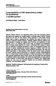
2.1 Annotating Use Case Diagrams A Use Case Diagram (UCD) provides a functional description of a system, its major scenarios (i.e., use cases) and its external users called actors (an actor may be a system or a person). It also provides a graphic description of how external entities (actors) interact with the system. Figure 1 presents a very simple UCD annotated for the reliability assessment purposes2 . In this case, two types of users and two use 1
Readers interested in UML basics can refer to [1]. Note that this type of UCD annotations have been used for performance assessment purposes in [2]. 2
303
P11
P12
Use case uc1
P21
Use case uc2
P22
User u1
User u2
q1
q2
Figure 1: Annotated Use Case Diagram. cases are considered. The annotations introduced are the same as in [9]: q1 and q2 represent the probabilities for users (or groups of users, each sharing similar system usage patterns) u1 and u2 , respectively, to access the system by requesting certain services. P11 and P12 represent the probabilities that user u1 requests the functionality f1 or f2 , respectively. P21 and P22 have a similar meaning with respect to user u2 . In general, the probability of executing the use case x is given by:
P (x) =
m X
qi · Pix
(1)
i=1
where m is the number of user types. Furthermore we assume that, for each use case, the set of all the relevant Sequence Diagrams (representing main scenarios within the use case) have been identified and specified. The assignment of use case probabilities, as in equation (1), infers that the same probability is assigned to the execution of every Sequence Diagram (SD) within the set corresponding to the use case. But in general, given a set of SDs, not all of them will have the same probability of execution. Hence, if we are able to assign a non-uniform probability distribution to the SDs referring to the same use case, equation (1) gives rise to the following equation [9]:
P (kj ) = P (j) · fj (k)
(2)
where fj (k) is the frequency of the k-th overall the SDs referring to the j-th use case. In our reliability model, presented in section 3, parameter P (kj ) represents the probability of a scenario execution.
2.2
Annotating Sequence Diagrams
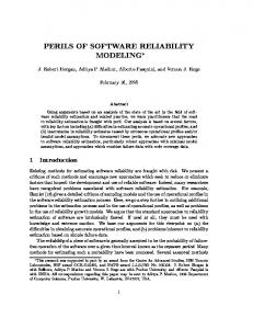
Sequence Diagrams (SDs) depict how groups of components interact to accomplish a given task. As mentioned in section 2.1, we assume that the behavior of each use case is given by a set of SDs. Interactions are drawn along a time axis, thus defining a partial order of execution. Hence, SDs provide specific information about the order in which events occur and can provide the information about the time required for reacting to events. When an interaction enters component’s axis (i.e., the component receives a service request), the component becomes busy. We therefore assume that a component is busy during interval of time that starts with an entering interaction and ends with the corresponding exit interaction [9]. In Figure 2, a Sequence Diagram specifically
C1
C2
C3 C1
l1
Figure 3: Annotated Deployment Diagram. ponents residing on the same site).
l2
Figure 3 shows an example of annotated Deployment Diagram including components in Figure 2. We number the failure probabilities over the connectors as ψ1 , ψ2 , etc., each corresponding to the failure probability of all the communications over the connector it is annotated on. Therefore, each pair of components (l, m) communicating over the connector i is subject to a failure probability ψi .
busy periods
l3 l4 l5
bp=1
bp=3
C3
psi
C2
l0
If we denote by |Interact(l, m, j)| the number of interactions that components l and m exchange in the SD j (note that this quantity is straightforwardly obtainable by visiting the SD), then the contribute ψlmj to the reliability of communication between these components (assuming it occurs over the connector i) in the scenario j is as follows:
bp=2
Figure 2: Annotated Sequence Diagram. annotated for our reliability model is shown.
ψlmj = (1 − ψi )|Interact(l,m,j)| .
It is easy to count the number of busy periods that component C i experiences in a given scenario (Sequence Diagram). For example component C3 in Figure 2 has two busy periods, the first one from the interaction labeled l1 to l2 , and the second one from l3 to l4 . In general, let us denote by bpij the number of busy periods that the component Ci shows in the Sequence Diagram j. If we assume that an estimate of the failure probability θi for every component Ci is available, then, as a first approximation, we can get the estimate of the probability of failure θij of the component i in the scenario j from the following equation [9]:
θij = P rob(f ailure of Ci in scenario j) = 1 − (1 − θi )bpij (3)
2.3 Annotating Deployment Diagrams A Deployment Diagram shows the platform configuration where the software application is targeted to run. Nodes represent platform sites (e.g., workstations, PCs, etc.) and links represents hardware/logical connectors (e.g., LAN, WAN, etc.). Additional boxes represent software components and are placed into the respective sites where they are supposed to be loaded. In practice this diagram shows the mapping of components to sites. The reliability of communication in distributed software can be critical, especially in unsafe environments. The annotation of a Deployment Diagram with the probabilities of failure over the connectors among sites (possibly a priori estimated) allows the reliability model to embed the communication failures. In fact, based on to these annotations a failure probability can be assigned to each interaction of a Sequence Diagram. The failure probability of an interaction between two remote components is the one over the connector linking the sites that host the components (it is reasonable to consider, as we do, fully reliable the communications among com-
304
(4)
Equation (4) takes also into account two special cases: • Two software components are co-located in the same platform site: the communication between them can be fairly considered totally reliable, because it does not involve any physical connection, that is ψi = 0 for these components. • Two components, wherever located, have no interactions: trivially it solves into |Interact(l, i, j)| = 0, bringing a neutral contribution 1 to the connection reliability product. One can argue that mapping of components to sites may not be available early in the lifecycle. In this case our model can nicely work without the contribution of communication failures (see [9]). However, if several mapping alternatives may be designed, equation (4) can be easily instantiated to produce the reliability of each alternative. In the latter case, the model may therefore support the comparison of different mappings based on reliability issues.
2.4
Combining component and connector failures
In order to build a formula for the reliability of the whole system, we here combine the failure probabilities of components (eq. (3)) and the ones of connectors (eq. (4)) as follows:
θS = 1 −
K X j=1
pj (
N Y i=1
(1 − θi )bpij ·
Y
(1 − ψlij )|Interact(l,i,j)| ).
(l,i)
(5) Equation (5) represents the mathematical formulation of our reliability model, and in section 4 we will apply it to our case study.
2.5 Model assumptions While defining this reliability model, we made several assumptions. First of them pertains to the existence of knowledge about failure rates for components and connectors. Traditional component libraries do not support this kind of information. However, we speculate that as libraries of reusable assets mature, information about failure histories could become available. Alternatively, component failure rates could, at a possibly high expense, be tested prior to the selection of an appropriate one. In an ideal futuristic scenario, we speculate that software COTS components could be sold with a specification sheet indicating their reliability information, much like is the case with electronic components are these days. Another simplistic assumption we make pertains to the independence of failures among different components. This assumption simplifies the modeling task. To some extent, proposals to build applications that include component wrappers, ensuring that the failure is caught in time and close to its source, make this assumption realistic [11]. At the expense of modeling ease, the independence assumption can be removed. Finally, we assume that component failures follow the principle of regularity, i.e., that a component is expected to exhibit the same failure rate whenever invoked. Note that equation (3) is only feasible under the above assumptions set on the estimate of component failure probabilities. Regularity and independence assumptions are further discussed below.
2.5.1
Regularity Assumption
Components may execute different tasks in different invocations. In an object oriented development environment, for example, the tasks that a component executes coincide with the methods (the entry points) of the component. A component handles a given type of incoming messages by executing the same method (determinism). Consequently, there is the potential to annotate every busy period of a Sequence Diagram with the name of the method being executed. Following this line of thinking, the unique θi of equation (3) can be replaced by a set of failure probabilities θil (l = l1 , ..., lbpij ), where each lk represents the method executed at the k-th busy period. Equation (3), in this case, becomes:
θij = P rob(f ailure of Ci in scenario j) = 1−
Y l=l1 ,...lbp
(1−θil ) ij
(6) For a preliminary estimate of θil , two cases may occur, depending on whether the source code of the corresponding method is available or not. If the source code is available, a preliminary estimate of θil may be obtained by statically analyzing the complexity of every component method. This approach assumes that method complexity can serve as a predictor of its failure rate. If source code is not available, estimates for component failure probability may be based on different model parameters. For example, Timed Sequence Diagrams may reveal the length of component’s busy period, and a (gu)estimate of component’s failure rate may depend on the duration of the execution. In a costly case, a method level testing could reveal an estimate of the failure rate upon demand. To us, these and other options for the assessment of individual methods appear to be an overkill. The issue is the granularity of the analysis and perceived gains in the precision of the reliability pre-
305
diction. We argue that if a component is tested as a unit with some understanding of the expected usage profile, the obtained failure probability should be a ”good enough” estimate. To further address this issue, our reliability prediction method accepts an uncertainty level (or confidence interval) describing component failure probabilities. Therefore, in our case study (see section 4) we adopt equation (3) as the basis for calculating θij .
2.5.2
Intercomponent Failure Independence
Another assumption we make pertains to the independence of failures among different components. Intercomponent failure independence implies that failures will not propagate from one component to another. The failures observed in different components become correlated when the components share state information. The state is composed of global variables, mutable data structures (passed parameters), shared memory, etc. Several system design rules can reinforce intercomponent failure independence. For example, safe programming languages (Java, ML, Ada) constrain the use of pointers, thus limiting the impact of shared memory to failure propagation. Global variables and mutable data structures can be checked at component interface with executable assertions. To some extent, proposals to build COTS based applications that include component wrappers, ensuring that the failure is caught in time and close to its source, make this assumption realistic [11]. The independence assumption simplifies the modeling task. This is the reason why all existing reliability models for component based systems assume it [5]. At the expense of ease, this assumption can be removed from our approach to reliability modeling, by introducing conditional component failure probabilities. In this case, component’s failure probability would depend on the sequence of components executed prior to its invocation. At this point in time, it is not clear whether the removal of the independence assumption automatically results in more accurate system reliability estimates. First and foremost, early in the development life-cycle, failure propagation probabilities are unknown and difficult, if not impossible, to estimate. Even if the reliability prediction framework accounted for a possible failure propagation, the associated probabilities could (and probably would) be inaccurate. Therefore, in the case study presented later, we assume intercomponent failure independence.
3.
A BAYESIAN RELIABILITY PREDICTION ALGORITHM
In [11] we proposed an algorithm based on Bayesian approach which incorporates the prior information about failure probabilities of components and known scenario probabilities for prediction of system software reliability. The algorithm has a straightforward extension to include the connector failure probabilities. Assume that θi s and ψlij s in (5) to be random variables having beta distributions with known parameters. The probability distribution of system failure rate, θS , can be obtained through simulation by generating random observations from the beta probability distributions of failure probabilities of components and connectors. The simulated probability distribution can be
used to predict the reliability of the system software even before the system testing results are available. Once the system testing results are available, these can be combined with the simulated distribution of θS for obtaining the posterior probability distribution of θS , which can be used to assess the reliability of the system software. We refer to [11] for details of the algorithm.
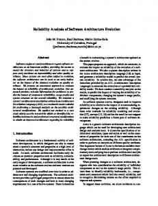
4. A CASE STUDY In this section we show, through a case study, annotated UML diagrams for an application, which is used, in turn, for reliability prediction. Annotations serve to build a reliability model, and the numerical results shown in this section support the claim of effectiveness and robustness of the proposed approach to reliability prediction of component based systems. We consider a simplified WEB-based transaction processing system, as in [9]. This system, illustrated in Figure 4, has been used as a case study also in [10].
PK
j=1
pj = 1 (see
Figure 6 illustrates one over four Sequence Diagrams that we have considered in this example, and it relates to the “remote write” use case (the other three diagrams related to “remote read” and “local operations” use cases can be found in [9]). It has been annotated with the number of busy periods for each component, following the approach described in section 23 . The values given to annotations in the Use Case Diagram of Figure 5 are the following: • user probabilities:
q1 = 0.8
q2 = 0.2 ;
• user to use case probabilities: P11 = 0.3 P21 = 0.1 P22 = 0.4 P23 = 0.5 .
P12 = 0.7
From equation (1) we obtain the probabilities for use cases, that are:
DB Local DB1
an occurrence probability pj , j=1,...,K, such that section 3).
Client 1
WEB Server Local DB2
Client 2 LAN
P(local operations) = p1 = 0.26
WAN INTERNET Remote Server
Remote Application Server Local DBn
P(remote read) = p2 = 0.64
Client n
P(remote write) = p3 = 0.10
Remote DB
Figure 4: WEB-based example.
P11
local operations
“local operations” and “remote write” use cases have only one scenario each, so p1 and p3 can be straightly used as scenario probabilities. Besides, by giving the same frequency to the two scenarios that the “remote read” use case has, p2 /2 = 0.32 will trivially be the probability of each one. Again, giving the same usage probability to the two “remote read” scenarios is a matter of choice, rather than the model limitation.
P21 P22
P12
remote read P23
low-level profile user q1
remote write
high-level profile user
Client C1
Web Server C2
q2 C4
psi1
C5
C3
C6 C7
psi2
Figure 5: Annotated UCD for WEB-BASED example.
Remote Server
Users, located on client nodes, have two different profiles: a so called low-level profile using the WEB connection only to carry out data search, and a high-level profile that is also enabled for remote data updates. The two user type frequencies of usage of the software system are denoted by q1 and q2 , respectively.
C10
Remote Application Server
C11
C8 psi3
C12
C9
Figure 7: Annotated DD. In Figure 5 an annotated UCD is shown [9]. From this diagram, different user profiles with related occurrence probabilities can be obtained as described in section 2. The probabilities on the edges between user must satisfy the following Ptypes and functionalities P conditions: 2i=1 P1i = 1 and 3i=1 P2i = 1. For each use case in the UCD, a set of execution scenarios (each of them represented by a different Sequence Diagram) is designed. A total of K different scenarios, corresponding to K different system behaviors, can are generated and each of them is characterized by
306
Figure 7 shows the annotated Deployment Diagram for our case study that straightforwardly comes from the organization shown in Figure 4 and the roles of software components introduced. 3 For lack of space, we do not provide many of the technical details needed to fully understand this case study. We hope that the chosen names of components and actions performed follow a selfexplaining criterion. Besides, since the reliability assessment is the focus, understanding all the application aspects might not be necessary.
main interface
User
client application
local DB
web interface
browser
web application
DB
request identif acc+passwd authoriz data request web data search web data search data process web data search processing web data search proc_reply web data found
proc_reply web data found data_search
web data found web data found create new page create new page create new page create new page
data_search data_search
new page ok new page ok
data_found new page ok data_found new page ok data_found
bp=5
bp=7
bp=3
bp=4
bp=1
bp=4
bp=4
bp=2
Figure 6: Annotated SD for “remote write” use case. Table 1 summarizes an annotation record for each component and connector of the case study. The first 13 rows represent components, the last 3 represent connectors. A component record includes the name of the component, the component failure probability and its 95% confidence interval, and the number of busy periods the component spends in each scenario. Note that the scenarios are numbered in the order they appear in the figures, from 1 through 4, and busy periods of a User are not reported because not used here. This also indicates that by simply allocating the busy periods to users (human or systems), they could be easily incorporated into the system level reliability analysis. A connector record of Table 1 includes the name of the connector, the connector failure probability and its 95% confidence interval. As from equation (5), the remaining parameter to be estimated is the number |Interact(l, i, j)| of interactions between components. Table 2 shows the number of interactions exchanged between components along the four scenarios considered (note that scenarios’ numbering follows the one in Table 1, and that we assume value 0 wherever no value is shown). It is easy to verify that these values have been obtained by simply counting the arrows in the Sequence Diagrams (the only exclusion from this table are the interactions between User and all the other components, because they are not based on a physical connector). Following equation (5), we can now formulate the failure probability for our case study as follows:
θS = 1− [0.26(1 − θ1 )6 (1 − θ2 )3 (1 − θ3 )+ + 0.32(1 − θ1 )4 (1 − θ4 )2 (1 − θ5 )2 (1 − θ6 )2 (1 − θ7 )(1 − ψ1 )2 + + 0.32(1 − θ1 )5 (1 − θ4 )3 (1 − θ5 )2 (1 − θ6 )2 (1 − θ7 )(1 − θ8 )2 (1 − θ9 )2 (1 − θ10 )2 (1 − θ11 )2 (1 − θ12 )(1 − ψ1 )2 (1 − ψ2 )2 (1 − ψ3 )2 + 0.10(1 − θ1 )7 (1 − θ2 )3 (1 − θ3 )(1 − θ4 )4 (1 − θ5 )4 (1 − θ6 )4 (1 − θ7 )2 (1 − ψ1 )4 ]. (7) We assume beta distributions with parameters ai and bi for component and connector failure probabilities. These parameters are given in Table 3 and these are based on prior information of failure probabilities of components and connectors given in Table 1. Simulation algorithm described in section 3 is used to generate 10,000 random observations on θS given by equation (7). A beta distribution is fitted to the normalized histogram of the generated observations. The normalized histogram along with the fitted beta probability density function is shown in Figure 8. The parameters of the fitted beta distribution are given by a = 228.94, b = 1313.21. The mean failure probability is 0.148. The functional form of the density is given by
h(θ) =
1 θ227.94 (1 − θ)1312.21 , 0 ≤ θ ≤ 1. B(228.94, 1313.21) (8)
Using this probability density function, a 95% credible (confidence) interval of θS is given by (0.131, 0.167). implying that a 95% con-
307
component/connector C1 C2 C3 C4 C5 C6 C7 C8 C9 C10 C11 C12 l1 l2 l3
Table 1: Information record of each component and connector. name failure confidence number of busy periods probability interval bpi1 bpi2 bpi3 bpi4 Main Interface 0.009 (0.006,0.012) 6 4 5 7 Client Application 0.005 (0.003,0.007) 3 0 0 3 Local DB 0.005 (0.003,0.007) 1 0 0 1 Browser 0.010 (0.007,0.013) 0 2 3 4 Web Interface 0.009 (0.006,0.012) 0 2 2 4 Web Application 0.005 (0.003,0.007) 0 2 2 4 DB 0.003 (0.001,0.005) 0 1 1 2 Remote Interface 0.009 (0.006,0.012) 0 0 2 0 Remote Application (RA) 0.005 (0.003,0.007) 0 0 2 0 RS Interface 0.039 (0.025,0.054) 0 0 2 0 RS Application 0.005 (0.003,0.007) 0 0 2 0 Remote DB (RS DB) 0.007 (0.003,0.010) 0 0 1 0 (Client, WEB Server) 0.009 (0.006,0.012) (Client, RA Server(RAS)) 0.009 (0.006,0.012) (RAS, Remote Server) 0.003 (0.001,0.005) -
Table 2: Number of interactions per pair of components overall the scenarios. pair (l,i) (C1 , C2 ) (C2 , C1 ) (C2 , C3 ) (C3 , C2 ) (C1 , C4 ) (C4 , C1 ) (C4 , C5 ) (C5 , C4 ) (C5 , C6 ) (C6 , C5 ) (C6 , C7 ) (C7 , C6 ) (C4 , C8 ) (C8 , C4 ) (C8 , C9 ) (C9 , C8 ) (C9 , C10 ) (C10 , C9 ) (C10 , C11 ) (C11 , C10 ) (C11 , C12 ) (C12 , C11 )
scenario 1 2 2 1 1
scenario 2
scenario 3
1 1 1 1 1 1 1 1
1 2 1 1 1 1 1 1 1 1 1 1 1 1 1 1 1 1
scenario 4 2 2 1 1 2 1 2 2 2 2 2 2
Table 3: The Values of Parameters of Prior Beta Distributions of the Component and Connector Failure Probabilities Component/Connector Failure Probability θ1 θ2 θ3 θ4 θ5 θ6 θ7 θ8 θ9 θ10 θ11 θ12 ψ1 ψ2 ψ3
ai 33.72 23.35 23.35 41.72 33.72 23.35 8.10 33.72 23.35 26.56 23.35 14.77 33.72 33.72 8.10
bi 3712.95 4646.65 4646.65 4130.28 3712.95 4646.65 1871.1 3712.95 4646.65 657.36 4646.65 2193.35 3712.95 3712.95 1871.1
ability density function of system software failure probability θS00 when the the failure probabilities θ11 and θ12 of the components C11 and C12 were increased by changing their mean failure probabilities to 0.02 and 0.025 with confidence intervals (0.01, 0.03) and (0.01, 0.04) respectively.
fidence interval of the reliability of the system software is given by (0.833, 0.869). The curves in Figure 9 have been plotted for investigating the effect of change of failure probabilities of some of the components on the system software reliability. The first curve gives the simulated probability density function of system software failure probability θS0 when the the failure probabilities θ5 and θ6 of the components C5 and C6 were reduced by changing their mean failure probabilities to 0.002 and 0.001 with confidence intervals (0,0.004) and (0,0.002) respectively. The third curve gives the simulated prob-
308
5.
CONCLUSIONS
In this paper we present an approach to the early validation of reliability in software modeled with UML diagrams. It is basically an extension of the model presented in [9] which does not consider failure probabilities over the connectors among components. The analysis framework is fully integrated with UML models, annotated to incorporate information about expected system usage patterns (a surrogate for an operational profile) and failure probability distributions of the components and the connectors used in the system.
Proc. of 2nd IEEE Workshop on Software and Performance (WOSP2000), September 2000. [3] W. Everett. Software component reliability analysis. In Proc. of Symposium on Application Specific Systems and Software Engineering Technology (ASSET’99), 1999. [4] S. Ghokale, M. Lyu, and K. Trivedi. Reliability simulation of component based software systems. In Proc. of 9th International Symposium on Software Reliability Engineering (ISSRE’98), 1998.
Figure 8: Plot of Prior Probability Density Function of the System Failure Probability θs fitted to the normalized histogram from simulation observations.
[5] K. Goseva-Popstojanova and K. S. Trivedi. Architecture-based approach to reliability assessment of software systems. Performance Evaluation, 45(2-3), June 2001. [6] J. Horgan and A. Mathur. Software testing and reliability. In Handbook of Software Reliability Engineering, pages 531–566, 1996. [7] S. Krishnamurthy and A. P. Mathur. On the estimation of reliability of a software system using reliabilities of its components. In Proc. of 8th International Symposium on Software Reliability Engineering (ISSRE’97), 1997. [8] B. Littlewood. Software reliability model for modular program structure. IEEE Transactions on Software Engineering, 28(3), 1979.
Figure 9: Plot of Prior Probability Density Function of the System Failure Probability θs in the three different experiments. This work opens numerous venues for further research. We are currently working on a set of automated tools to accompany the proposed methodology. The tools will be accessible from UML diagrams, making them potentially very attractive to a wide audience of software developers. An interesting possibility for model extension is the introduction of imperfect system users in terms of their reliability, i.e., knowledge about the appropriate system usage. Imperfect users are the fact in the real world applications. Use cases provide a natural modeling environment for this extension.
6. ACKNOWLEDGMENTS This work was supported in part by the NSF award CCR-0093315 and in part by NASA through cooperative agreament NCC 2-070. The opinions, findings, conclusions and recommendations expressed herein are those of the authors and do not necessarily reflect the views of the sponsors.
7. ADDITIONAL AUTHORS Additional authors: Erdogan Gunel (Department of Statistics, West Virginia University, email:
[email protected]) and Vijay Bharadwaj (Department of Computer Science and Electrical Engineering, West Virginia University, email:
[email protected]).
8. REFERENCES [1] http://www.rational.com/uml. [2] V. Cortellessa and R. Mirandola. Deriving a queueing network based performance model from uml diagrams. In
309
[9] H. Singh, V. Cortellessa, B. Cukic, E. Gunel, and V. Bharadwaj. A bayesian approach to reliability prediction and assessment of component based systems. In Proc. of 12th International Symposium on Software Reliability Engineering (ISSRE’01), 2001. [10] C. Smith. Spe for web applications: New challenges? In Keynote Address in Proc. of 2nd International Workshop on Software and Performance (WOSP2000), 2000. [11] J. M. Voas. Cots and high assurance: An oxymoron? In Proc. of 4th IEEE International Symposium on High-Assurance Systems Engineering (HASE’98), 1998. [12] M. Xie and C. Wohlin. An additive reliability model for the analysis of modular software failure data. In Proc. of 6th International Symposium on Software Reliability Engineering (ISSRE’95), 1995. [13] S. Yacoub, B. Cukic, and H. Ammar. Scenario-based reliability analysis of component-based software. In Proc. of 10th International Symposium on Software Reliability Engineering (ISSRE’99), 1999.