Early-spring export of phytoplankton production in the ... - Inter Research

Vol. 114: 197-202, 1994

MARINE ECOLOGY PROGRESS SERIES Mar. Ecol. Prog. Ser.

1

Published November 3

NOTE

Early-spring export of phytoplankton production in the northeast Atlantic Ocean Cheng Ho, John Marra Lamont-Doherty Earth Observatory of Columbia University. Palisades, New York 10964. USA

ABSTRACT: Detailed observations of water column temperature a n d phytoplankton biomass in the northeast Atlantic Ocean prior to the advent of the spring bloom in 1989 show brief periods of water column stabilization and phytoplankton production, interspersed with times where temperature and biomass are constant over greater depths Since stable layers re-form from the surface, the observed variability in mixed layer depth is analyzed as isolating phytoplankton beneath the euphotic zone, potentially contributing to the annual exported produchon in the temperate North Atlant~c.

KEY WORDS: Phytoplankton . Mixing . Export. Mixed layers

The North Atlantic is noted for a strong seasonal cycle in the productivity of the plankton and for the vertical flux of biogenic material to the deep sea, with the strongest signal for each of these in spring (see e.g. Ducklow & Harris 1993). Two concepts govern thinking with regard to this seasonal cycle: (1) that phytoplankton can only accumulate in the surface layer if the depth to which the water column is stable is less than the depth for which water column photosynthesis balances losses (Sverdrup 1953); and (2) that the majority of the flux of biogenic material out of the euphotic zone is through growth or suspension feeding (Bishop 1989). Here we discuss how an extension of the first concept might influence consideration of the second. We present data which point to a potentially important loss term for phytoplankton, resulting as a consequence of variations in the mixed layer depth. That loss of phytoplankton occurs through the dynamics of mixed layers is not new. For example, it has been treated theoretically by Woods & Onken (1982) for the diurnal time scale and Platt et al. (1991). However, the implications of mixing-induced losses to export have perhaps not been appreciated (Gardner O inter-Research 1994

Resale o f full article not permittea

et al. 1993, cf. Hill 1992), let alone observed. Here, we derive a simple relationship to examine the phenomenon, and show data from a recent experiment in the North Atlantic. Finally, we mention some indirect support for the idea that the time period prior to the spring bloom may contribute significantly to export of primary production in seasonally varying ocean ecosystems. Analysis. The seasonal cycle in the North Atlantic Ocean is a cycle of stratification, but that stratification is episodic, especially early in the season (Bishop et al. 1986). Mixed layers will deepen, a process induced by the wind and by heat loss to the atmosphere (Price et al. 1986). but they do not shoal. Instead, the surface warms, and depending on conditions, a new mixed layer will re-form from the surface. Thus, mixed layer cycles of stratification and re-stratification are discontinuous in time with implications for phytoplankton production and export to depth. We illustrate the way in which mixed layer deepening can enhance the vertical flux of phytoplankton using 2 derivations for the balance of chlorophyll a (a measure of phytoplankton biomass) in the upper layers where sinking dominates loss to production. In the first case, assume that the water column can be divided into 2 layers (Fig. l a ) . At any time t, the phytoplankton in the top, mixed, layer of depth M is designated as Chll, and the phytoplankton in the bottom layer as Chl,,. At a time At later, the mixed layer depth is M+AM, and the phytoplankton layers are Chll +AChl, and Chill +AChlll. In the limit, the balance of chlorophyll can be expressed as dM dt

dChll M + (Chl, - Chl,,)--

dt

=

I.

M

cdr

(1)

for dM/dt > O , where c is the rate of production of chlorophyll.

Mar. Ecol. Prog. Ser. 114: 197-202. 1994

S.

Chl

Fig. 1. Schematic of 2 formulations for the l-dimensional balance of chlorophyll in the surface layers of the ocean. (a) Case 1, the balance for 2 layers, where the top layer increases by AM. (b) Case 2, the balance for 1 layer, with a constant sinking rate, s

The second case is a volume of water containing chlorophyll (Fig. l b ) . The change in chlorophyll will be balanced by production and loss by sinking, S. The balance of chlorophyll in this case can be written as

where A V = m y A z . Dividing both sides by A V and taking the limit as A V - 0 leads to

-a Chl at

-

C-S-

a c~ a2

We now assume a layer similar to the mixed layer identified in the previous case, M = M ( t ) . Integrating over hl,

leads to

I

M

JoM

dz + r ( ~ h l ( 0-)C h l ( ~ )=]

0

cdz

(2)

Eq. (2) has been derived before (e.g. Taylor et al. 1992, Taylor & Stephens 1993) except that here we have neglected mixing across the layer boundaries. Although in case 1, sinking was neglected, the resulting equations for the 2 cases are very similar. The right side of each, the production term, is the same. The first

term on the left side of each has the same physical meaning, except that in Eq. ( l ) ,Chl, represents the phytoplankton mixed over M, while in Eq. (2), no assumption has been made about the distribution within the volume. The second terms in each equation are also different, and suggest a mechanism for the vertical flux. Both indicate the difference of chlorophyll between the top and bottom of the respective layers, suggesting that dMldt is equivalent to s. Thus, the deepening of the mixed layer can be seen as equivalent to a sinking rate. Mixed layers can deepen by tens to hundreds of meters per day, making dMldt 2 to 3 orders of magnitude greater than sinking rates of large cells, i.e. those with the highest sinking rates in laboratory measurements (Smayda & Boleyn 1966). Comparatively speaking, the deepening of the mixed layer may be an important loss mechanism. We can also establish some limits on the above analysis. Eq. (1)applies only where mixed layer depth increases. A persistent, deep mixed layer is not efficient for the export of phytoplankton. Indeed, all processes are slowed (Sverdrup 1953).The most effective way to mix chlorophyll down is to have a shallow mixed layer and high production rates during the day with mixed layer deepening at night. That is, if we assume that s = dM/dt, it is possible, using the above equations, to derive an optimum for the flux which corresponds to a minimum M with a maximum rate of production, i.e. the diurnal cycle of photosynthesis and mixing. A diurnal cycle of stratification and mixing great enough to achieve the optimum, however, is not typical. Passing weather systems may keep a mixed layer deep or shallow for days at a time, and after seasonal stratification, continued positive heat flux will cause a mixed layer more resistant to vertical mixing. Properties of the diurnal mixed layer for phytoplankton production have been explored elsewhere (e.g. Taylor & Stephens 1993, and references cited therein). Evans & Parslow (1985) noted a similar dynamic to the above analysis in their parameterization for the seasonal variability of mixed layer depth. In their model, phytoplankton (and nutrients) are diluted by a deepening mixed layer but are unaffected otherwise. An example. Data to support the above mechanism are difficult to obtain since the process requires that we discern local from advective effects. While this can never be absolutely ascertained, the use of moored observations (as opposed to sequential profiles from on board ship) increases the time resolution of the phenomena for improved interpretation. Nevertheless we believe we have identified one or more deepening events in data obtained from moored sensors in the northeast Atlantic Ocean in early spring 1989 (see Fig. 2) which illustrates mixing-induced loss.

Ho & Marra Early-spring export

Fig. 2. An area of the northeast Atlantic Ocean, the site of the Marine Light-Mixed Layers (ML-ML) Program (Marra 1989), showing the position of the mooring at 5g0N,21°

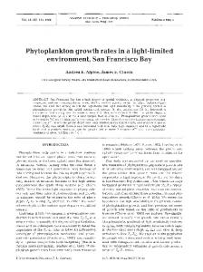
High frequency sampling of water column properties was done from the mooring which recorded meteorological variables at the surface, and physical (current velocity, temperature) and bio-optical properties [fluorescence, transmissivity, irradiance (PAR), dissolved oxygen] at 10, 30, 50, 90, 110, and 250 m in the water column from mid-April to June 1989 (see Stramska & Dickey 1992). The fluorescence sensors were calibrated against chlorophyll a as described previously (Marra et al. 1992, Marra & Langdon 1993). We determined mixed layer depth in 2 ways, as generated by the mixed layer model of Price et al. (1986),the inputs for this model coming from the mooring meteorological data, and as calculated by interpolating the temperature between the depths where the moored thermistors were located. Both of these are approximations. The model is 1-dimensional, thus spatial variability in wind and surface advection can result in error. The moored sensors, on the other hand, spaced 10 to 20 m, are too far apart for optimal depth resolution in temperature. Current velocities average about 25 cm s , or about 20 km d ' (Fig. 3a). Thus over a 5 d period, the data represent conditions occurring over 100 km, about the scale of ocean eddies. Large oscillations are apparent in mixed layer depth on Days 106 to 108 (April 14 to 16), and are more apparent in the mixed layer depth models than that estimated by the moored thermistors (Fig. 3b). Oscillations occur because, as stated above, stratification forms from the surface. The model records intermittent stabilization of the water column from solar heat flux and low winds. The water column is subsequently mixed over deeper depths at night. Otherwise the observations do not indicate a flow- or eddy-dominated regime such as has been suggested for later in the season at these latitudes (Woods 1988). The data suggest a change from this early period of die1 stratification and mixing on about Day 108. For about 4 d, the mixed layer depth remained shallower than about 50 m, allowing an increase in chlorophyll

1

199

mixed layer depth (m)

b

1

Julian Day 1989 Fig. 3. Moored sensor data. (a) Current velocities shown only at 10 m depth, however, these coincide with the other current meter records for depths down to 250 m. Bar indicates 25 cm s". (b) Mixed layer depths, calculated from the output of a mixed layer model (Price et al. 1986) using the criterion of a 0.1 OC temperature difference between the surface values and that at depth (dotted line) and from the temperature differences in the moored thermistors using the same criterion (solid line), (c) Contours of chlorophyll fluorescence (mg chlorophyll a m 3 ) . (d) Temperature data from the moored thermistors. Other data from this mooring experiment are presented in Stramska & Dickey (1992)

biomass (Fig. 3c). Subsequently, the mixed layer deepened at a rate of 50 m d l , although radiative flux during a few of the days may have been sufficient for daytime stabilization. Phytoplankton growth continued, accompanied by a flux to deeper water (Fig. 3c).

Mar. Ecol. Prog. Ser 114. 197-202, 1994

200

An apparent export of chlorophyll to deeper depths was visible throughout the period of Days 114 to 120, after which a change in the current pattern and wind led to much deeper mixing. Chlorophyll concentration dropped by 40 % by Day 120. If not the absolute magnitude, at least the proportion of production lost by this process can be estimated and thereby its potential importance can be assessed. The calculation will be necessarily rough because we do not have independent physiological data on growth or photosynthesis, and because we have to make an assumption regarding the depth beneath which chlorophyll is lost from the productive layer. The loss at depth is analogous to that which might be collected in a sediment trap at a fixed depth. We calculate the loss of phytoplankton cells from the surface layer assuming Eq. (1) describes the balance of chlorophyll and assuming that the chlorophyll flux through 100 m depth is lost from the system, 100 m being twice the depth of the usual spring and summer mixed layer and euphotic zone. We use the criterion for the depth of the mixed layer of a 0.1 "C change from the surface value, a value that is conservative for the calculation of the flux. The net production, c, is estimated from in situ changes in chlorophyll for the days in which chlorophyll is seen to increase, i.e. Days 109 to 111 (Fig. 4), along with data from the mooring PAR sensors to generate net production of chlorophyll as a function of irradiance. The resulting relationship has only 3 points, corresponding to the depths at which we have sensors (Fig. 5), however they represent data averaged over 3 d (Fig. 4). The advantage of using the in situ changes

0 109

l l0

Ill

112

Day, 1989 Fig. 4 . Chlorophyll a as measured by the moored fluorometers for Days 109 to 111 (when the water column was stratified) (solid line: 10 m; short-dashed line. 30 m, long-dashed Ilne. 50 m ) . The straight lines are linear regressions of the data The regression coeff~cientswere taken as estimates of the chlorophyll product~on over the 3 days considered here (see Fig. 5)

0

20

40

60

80

100

Avg. Irradiance (~Einsteinsm-2 S-') Fig. 5 . Photosynthesis-irradiance relationship used in the calculations. The symbols are the daily-averaged rate of chlorophyll production for Days 109 to 11 1, as shown in Fig. 4 . Irradiances are averaged over the 3 days and presented as instantaneous fluxes. The line is f(1)= 0.134 tanh (1/25),where 0.134 is the highest observed rate of chlorophyll production and 25 is a fitting parameter (equivalent to Ik, e.g. Chalker 1980)

in chlorophyll is that we have a direct measure of net production, averaged over a few days (see below). One disadvantage is that the net production estimates and the time step of the model are temporally mismatched. Going to shorter-term (i.e. hourly) estimates of net production, however, introduces other factors which are difficult to parameterize, such as day-night differences in respiration, and photoinhibition of fluorescence (see Marra 1992). The calculation is initialized using the chlorophyll values at the 3 depths at the beginning of Day 109 and a mixed layer of 10 m. We compute the mixed layer depths as generated by the model of Price et al. (1986) (see Fig. 3). The PAR data is used to calculate the net production of chlorophyll (Fig. 5 ) . The model uses a time step of 1 h, and production is summed over each day and depth. The redistribution of chlorophyll is based on the change in mixed layer depth according to E q . (1). From our calculations, area1 net production remained relatively constant throughout Days 109 to 122 at 1.5 to 2 mg chlorophyll m-' d-l. Overall, computed net chlorophyll production was 88 mg m-', and the flux at 100 m is 44 mg chlorophyll mT2through mixing, or 50% of production. Sinking losses, depending on the choice of sinking rate (0.1to 3 m d-'; Smayda & Boleyn 1966) will account for an, additional 2 to 10%. Using a carbon:chlorophyll ratio of 40 (by weight), the production is about 300 mg C m-' d-l, a value not atypical

Ho & Marra: Early'-sprlng export

for the northeast Atlantic in early spring (unpubl. results). Clearly, in this rough calculation we have not accounted for losses such that the observed stable quantity of chlorophyll is maintained in the surface layers. It is not clear over what time period a budget such as this will apply and therefore reduce errors from local advection, from the definition of the mixed layer depth, the assumption of a fixed depth-horizon for loss, and from the simple representation of net production. Nonetheless, the magnitude of the loss from mixing suggests that this is an important process during the period prior to seasonal stratification of the water column. Others have implicated mixing as an agent for export production. For example, successive mixing events in late winter and early spring in a warm-core ring contribute to export beneath the euphotic zone of as much as 67 % of primary production (Bishop et al. 1986). To explain the variability in particle profiles, Gardner et al. (1993) construed a 'mixed-layer pump' as a mechanism for export from the surface layer. C. Stienen (pers. comrn.) noted a pulse of chlorophyll in sediment traps deployed at 350 m, well before the advent of the spring bloom in 1989 (see Marra & Ho 1993). Other evidence suggests the importance of intermittent stabilization of the water column prior to seasonal stratification. For example, according to model calculations, removal of nitrate equal to 50% of the spring bloom utilization occurred earlier than the observed seasonal stratification of the water column in the North Atlantic (Garside & Garside 1993). Satellite imagery of continental shelf waters often shows intermittent concentrations of chlorophyll during winter (Yoder et al. 1993), which may be indicative of the dynamics we have seen from the moored data. Mixed layer deepening, i.e. a mixing-induced flux may explain the above observations of export production in the open ocean. It is also a mechanism which does not require (but does not rule out) particle aggregation to achieve fluxes necessary to match that implied by sediment trap collections (Hill 1992). Rapid vertical flux has been shown to be important to herbivores living at depth (Bishop et al. 1986, Sasaki et al. 1988) and, during late winter, we may speculate that flux events such as the one described here trigger the seasonal development of copepods so that their reproduction coincides with the spring bloom. Mixing and re-stratification cycles afford direct control of particle abundances in the upper layers, and therefore control optical variability. Data from the North Atlantic supply the evidence here, however, the mixing-induced flux should apply to other regions where rapid deepening of the mixed layer can occur. Events prior to seasonal stratification may be just as significant to annual export production as that associated with the spring bloom.

20 1

These observations suggest a different perspective on plankton dynamics in early spring. For the period prior to the spring bloom in the North Atlantic, critical depth analysis (Sverdrup 1953) implied no growth at the daily time scale. This idea should be extended to include growth punctuated by loss to depth, with effects on optics, herbivores, and mechanisms of the vertical transport of particles.

Acknowledgements. The mooring observations were a joint effort between T. Dickey (USC) and J.M. We are grateful for comments from J . K. B. Bishop and for the assistance of a n anonymous reviewer. Supported by the Office of Naval Research grant N00014-89-5-1150. This is LDEO contribution no. 5261.

LITERATURE CITED Bishop, J . K. B. (1989). Regional extremes in particulate matter composition and flux: effects on the chemistry of the ocean interior. In: Berger, W. H., Smetacek, V. S., Wefer. G. (eds.) Productivity of the ocean: present and past. John Wiley & Sons, Ltd, Chichester, p. 117-137 Bishop, J. K. B., Conte, M. H., Wiebe. P. H.. Roman, M. R., Langdon, C. (1986). Particulate matter production and consumption in deep mixed layers: observations in a warm-core ring. Deep Sea Res. 33. 1813-1841 Chalker, B. E. (1980). Modelling light saturation curves for photosynthesis: an exponential function. J theor. Biol. 84: 205-215 Ducklow, H. W., Harris, R. P. (1993). Introduction to the JGOFS North Atlantic Bloom Experiment. Deep Sea Res. 40: 1-8 Evans, G. T., Parslow, J. S. (1985). A model of annual plankton cycles. Biol. Oceanogr. 3: 327-347 Gardner, W. D., Walsh, 1. D., Richardson, M. J . (1993). Biophysical forcing of particle production and distribution during a spring bloom in the North Atlantic. Deep Sea Res. 40: 171-195 Garside, C., Garside, J . C. (1993).The 'f-ratio' on 20" W during the North Atlantic Bloom Experiment. Deep Sea Res. 40: 75-90 Hill, P. S. (1992). Reconciling aggregation theory with observed vertical fluxes following phytoplankton blooms. J. geophys. Res. 97: 2295-2308 Marra. J. (1989). Bioluminescence and upper ocean physics: seasonal changes in the Northeast Atlantic. Oceanography 2: 36-38 Marra, J . (1992). Diurnal variability in chlorophyll fluorescence: observations and modelhng. In: Gllbert, G . D. (ed.) Ocean Optics XI. Proc. SPIE, Vol. 1750. The International Society for Optical Engineering (SPIE), Bellingham, WA, p. 233-244 Marra, J . , Dickey, T., Chamberlin, W. S., Ho, C., Granata, T., Kiefer, D. A., Langdon, C., Smith, R., Baker, K., Bidigare, R., Hamilton. M. (1992) The estimation of seasonal primary production from moored optical sensors in the Sargasso Sea. J . geophys. Res. 97: 7399-7412 Marra, J.. Ho, C. (1993). Initiation of the spring bloom in the northeast Atlantic (47' N, 20" W): a numerical simulation. Deep Sea Res. 40: 55-73 Marra, J . , Langdon, C. (1993). An evaluation of an in situ fluororneter for the estimation of chlorophyll a. Tech.

202

Mar. Ecol. Prog. Ser. 114: 197-202, 1994

Rep. LDEO-93-1. Lamont-Doherty Earth Observatory, Palisades. NY Platt, T., Bird, D. F., Sathyendranath, S. (1991). Critical depth and marine primary production. Proc. R. Soc. Lond. B 246: 205-217 Price, J . , Weller, R. A., Pinkel, J . (1986). Diurnal cycling: observations and models of the upper ocean response to diurnal heating, cooling and wind mixing. J. geophys. Res. 91: 8411-8427 Sasaki, H., Hattori, H., Nishizawa, S. (1988). Downward flux of particulate organic matter and vertical distribution of calanoid copepods in the Oyashio Water in summer. Deep Sea Res. 35: 505-515 Smayda, T. J., Boleyn, B. J. (1966).Experimental observations on the flotation of marine diatoms. 111. Bacteriastrum hylaninum and Chaetoceros lauden. Limnol. Oceanogr. 11: 35-43 Strarnska, M , , Dickey, T. (1992). Variability of bio-optical properties of the upper ocean associated with die1 cyles in phytoplankton population. J . geophys. Res. 97: 17873-17887 Sverdrup, H. U. (1953).On conditions for the vernal blooming

of phytoplankton. J. Cons. Explor. Mer 18: 287-295 Taylor, A. H.. Stephens, J. A. (1993).Diurnal variations of convective mixing and the spring bloom of phytoplankton. Deep Sea Res. 40: 389-408 Taylor, A. H.,Watson, A. J . , Robertson, J . E. (1992).The influence of the spnng phytoplankton bloom on carbon dioxide and oxygen concentrations in the surface waters of the northeast Atlantic during 1989. Deep Sea Res. 39: 137-152 Woods, J. (1988). Scale upwelling and primary production. In: Rothschild, B. J. (ed.) Towards a theory of biologicalphysical interaction in the ocean. D. Riedel, Dordrecht, p. 7-38 Woods, J . D., Onken, R. (1982) Diurnal vanation and primary production in the ocean - preliminary results of a Lagrangian ensemble model. J. Plankton Res. 4: 735-756 Yoder, J A., Brown, C. W., Garcia-Moliner, G., Stegmann, P. M. (1993).Scientific applications of sea wide field sensor (SeaWiFS) imagery. In: Proceedings of Environment 93, Symposium on remote sensing m environmental research and global change. The Commercial Press, Hong Kong, p. 46-58

This note was submitted to the editor

Manuscript first received: September 20, 1993 Rewsed version accepted: July 27, 1994