Economics of Software Verification Gerard J. Holzmann Bell Laboratories MH 2C-521 600 Mountain Avenue Murray Hill, NJ 07974
[email protected] ABSTRACT How can we determine the added value of software verification techniques over the more readily available conventional testing techniques? Formal verification techniques introduce both added costs and potential benefits. Can we show objectively when the benefits will outweigh the cost?
Categories and Subject Descriptors D.2.4 [Software/Program Verification]: Formal methods, validation F.3.1 [Specifying, Verifying, and Reasoning about Programs]: Mechanical verification.
General Terms Algorithms, Measurement, Design, Reliability, Verification.
Keywords Model checking, software verification, testing, Spin.
1. INTRODUCTION No single system of metrics for measuring software quality is universally accepted [4,5]. Intuitively, software quality is related to the ratio of the perceived usefulness of a product and its perceived buggyness. The usefulness of a product is related to its functionality, which is in turn related to code size. More functionality often implies more code. As a metric for buggyness one often uses the elusive standard of ‘residual defect density.’ The residual defect density is meant to measure the number of defects that remain in a software artifact after delivery to the enduser (the customer), weighted by code size. A typical target in software development is to achieve a residual defect density of less than one defect per one thousand lines of non-comment source code [4,10]. Though most programming teams strive for zero residual defect density, it would be unrealistic to assume that product testing can proceed until this goal is fully reached. It can already be very hard to determine if the goal is ever reached. As Edsger Dijkstra noted, the inability to locate further defects does not necessarily imply the absence of defects. Residual defects almost always exist, even for the most vigorously tested code [1,9,10,12]. Permission to make digital or hard copies of all or part of this work for personal or classroom use is granted without fee provided that copies are not made or distributed for profit or commercial advantage and that copies bear this notice and the full citation on the first page. To copy otherwise, or republish, to post on servers or to redistribute to lists, requires prior specific permission and/or a fee. PASTE’01, June 18-19, 2001, Snowbird, Utah, USA. Copyright 2001 ACM 1-58113-413-4/01/0006…$5.00.
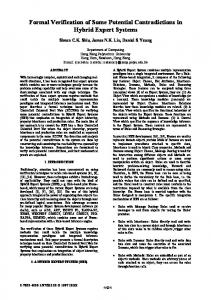
The residual defect density of a software product can often only be estimated, based on the number of user complaints. The number of complaints does not just depend on the residual defect density, it also depends on the number of users, and the amount and duration of actual usage. Different metrics can be used to determine when a product is ready to ship. Not surprisingly, the most commonly used metric is not related to zero defect density but to the cost that is associated with the search for residual defects, and the relative effectiveness of that search. Finding bugs can be likened to finding randomly distributed Easter eggs in a large meadow. Figure 1 can be interpreted as a plot of the cumulative number of eggs found, as a function of time. After an initial orientation phase, the rate at which eggs are found will tend to be a linear function of the amount of time spent searching. The area that can be searched per unit of time will roughly be constant, and if eggs are distributed uniformly, the rate at which they are found will also be constant. But the search process is not perfect, and some areas may need to be searched again, presumably more carefully than at first. As the number of residual eggs drops, the amount of time that has to be spent to locate them increases. The search becomes less effective and at some point it will have to be called off, even if it is known that not all eggs were found. Due to its characteristic shape, this curve is often referred to as the S-curve of software testing, cf. [11].
cumulative number of defects found cutoff point
time spent testing
Figure 1. The characteristic S-curve for defect removal. To measure the effectiveness of the search process, let us assume a fixed search cost of n dollars per minute. Let us further assume that there is a fixed reward of m dollars for each egg found. If we are finding r eggs per minute, it will pay to continue searching
only as long as r× m > n. The only thing worthwhile observing in this is that there is indeed a cutoff point where the cost of searching will start exceeding the expected benefit. In software testing there is of course no direct reward for every bug found, but only a potential penalty for every bug missed by the tester and found by the customer. The trade-off remains as before. If the probability that a customer finds a bug is p and the average associated penalty is q dollars, then the estimated cost of a missed bug is p×q dollars, and our metric for continuing the search becomes p×q > n, in line with the earlier formula. At some point it is no longer practical to continue the search for residual software defects. This, at least, is the conventional wisdom.
2. THE PRICE OF DEFECTS Not every defect is equally damaging, and it may be a bit too simplistic to consider only the average cost associated with bugs, as we have done so far. There is no real hard data to fall back on here for an assessment of how the severity of bugs correlates with bug density, but we can formulate a hypothesis. West [13] classifies defects into levels based on the number of independent factors that are jointly required to cause their occurrence. In this classification, a defect triggered by a single cause is called a defect of level one. A defect of level two has two independent causes that must occur in a particular combination. The first cause could be the failure of a standard routine (“cannot write – disk full”), and the second cause could be the failure of the exception handling routine that is invoked to recover from the first failure. Similarly, a defect of level ten would require ten independent failures to occur in a specific combination. Clearly, the higher the level of a defect, the less likely its occurrence will be [2,4,6,13]. We can now formulate the hypothesis that the defect level of potentially catastrophic failures, say the ones that can cause a complete system failure, is relatively high, requiring multiple things to fail in combination. If true, high impact failures will tend to have a lower than average probability of occurrence, and are more likely to survive traditional testing. The predicted effect is illustrated in Figure 2.
The tail of the curve, corresponding to software defects with small probabilities but large potential impact, can in principle reach arbitrarily far. There is no simple bound here that could be derived from product specifics. After all, also a ten-dollar product can conceivably cause a million dollars in damages, if catastrophically faulty We now return to the S-curve from Figure 1. The cutoff point in Figure 1 is reached when a particular number of software defects has been found. As noted, this point is reached when the rate at which defects are detected drops below a pre-determined limit. If our assumption is valid that bugs are found approximately in order of their probability of occurrence, we can indicate the cutoff point also in Figure 2. The less likely bugs take longer and longer to detect. It therefore seems plausible that the rate at which bugs are detected in conventional testing is correlated with their probability of occurrence. If this is indeed the case, we should expect the population of residual software defects to be skewed towards the higher-impact defects with a lower probability of occurrence. We can find some further support for these observations in the literature. Studies have been done, for instance, in which the defect densities for frequently used code are compared with that for rarely user code. Presumably rarely used code (e.g., exception handling code) contributes defects with a lower probability of occurrence and frequently used code contributes more towards the high probability flaws. One study reported the following results for a telephone switching system. “The fault density computed from test results indicated that the rarely executed segments had fewer faults than frequently executed ones, but in operation the order reversed, even though the frequently executed segments experienced very much more execution time. As might be expected, the failures in the frequently executed code occurred earlier during the operational period; rarely executed code took much longer to get debugged and probably still contained many residual faults at the end of the first year.” [6] Elsewhere the same report notes that the rarely executed code was a significant factor in determining product quality as perceived by the end-user: “The size of the [rarely used] code was 20% less than the [frequently used code], but it contributed 2.5 times more to the post-release failures that brought the system down.”
number of defects
cutoff point
less likely / more impact
Figure 2. Risk and damage: low-impact defects tend to occur more frequently than high-impact defects.
There is also a relation between perceived defect density and the average number of users of a product. Here the irony of successful product development comes into play. The more successful a product is, the more users it has, and the more likely it is that even unlikely defects will eventually be noticed. Since estimates of residual defect density are typically based on the number of customer complaints post-release, successful products would appear to have a higher residual defect density than unsuccessful products. Statistics on product recalls for non-software products can illustrate the existence of this phenomenon. The New York Times, for instance, reported data from the Consumer Product Safety Commission on recalls for nine different brands of a particular type of baby seats [14]. The data, reproduced graphically in
Figure 3, includes the number of units that were sold for each brand of baby seat at the time of the recall, the number of complaints received and the number of injuries reported. Injuries can result from rare, though no less dramatic, sequences of events. (For instance, a baby falling from the seat on a hard surface, when the handle breaks and the child restraint fails.) At first sight it would appear that Figure 3 shows that the most popular products are of the poorest quality: they have the largest number of reported defects. In reality though, the likelihood of rare combinations of events occurring increases with the number of users of the product, whatever the product may be. The four million users of product brand 9 will collectively encounter far more problems than the six thousand users of brand 1, also if the two brands are of comparable quality. This is as true for software products as it apparently is for baby seats. 10000000
1000000
100000
10000 # Users # Complaints # Injuries 1000
100
10
can expect, for instance, that if the residual software defect density increases, customer satisfaction decreases. If the number of defects encountered by the customer increases beyond a certain level, we can expect that customer satisfaction will drop so low that the users will avoid using the product. The above assumes that our starting point is complete customer satisfaction, with the target customer unaware of any defects in the product. If the starting point is different, for instance if the target customer assumes a buggy product, based on past experience, it will be harder to re-establish customer satisfaction. A curve that plots customer satisfaction against residual defect density, therefore, will likely exhibit hysteresis (capturing the notion that customers have memory and are affected by past experiences). An attempt to capture these notions is shown in Figure 4. If we start at the point labeled 1 on the upper curve in Figure 4, and slowly move towards point 2, small changes in the residual defect density do not seem to affect customer satisfaction all that much. When we pass 2, though, the effect will become very noticeable. Similarly, is we start on the lower curve at 3 and move towards 5, small changes in residual defect density do not cause easily observable effects, not even if we pass 4, restoring the same residual defect density we had before we started losing users at point 2. Any improvement in defect density will now have to be considerably greater, before it can restore customer confidence that the product is worth using. (It might explain why many companies often decide to abandon a product at this point, rather than attempt to restore lost customer confidence.)
1 1
2
3
4
5
6
7
8
9
Figure 3. Correlation between the number of users and the number of reported defects for nine brands of baby seats subject to recalls [14]. (Connecting lines not part of the data.) The conclusion is not that the amount of testing that is required for a product should depend on an estimate of the eventual number of users. Even a small number of users will eventually stumble upon the problems that remain in the code. If one is interested in building healthy long-term relations with users, it is worth avoiding also the long-term disappointments. It has been said that:
customer satisfaction 1 satisfied customers
unsatisfied customers (lost sales)
5
2
4
3
“A high fault density is more likely to be an indicator of extensive testing than of poor quality.” [3] defects found by customer
The corollary, based on Figure 3, would be: “A low residual defect density is more likely to be an indicator of a small user population than of high product quality.” Perhaps more to the point, we can conclude that the often-used metric of residual fault density is a relatively poor estimator of product quality and of the adequacy of a testing effort. The relations are more subtle.
3. CUSTOMER SATISFACTION The search for bugs gradually becomes less effective and more expensive with time. But, we have not yet taken into account the end-user’s resilience to bugs. The user is willing to accept a mild level of defects, as long as they can easily be worked around and are fixed when reported. We can speculate a little on the relation between customer ‘satisfaction’ and residual software defects. We
Figure 4. Changes in customer satisfaction as a function of changes in residual defect density.
4. DEFECTS AND FEATURES So far we have conveniently assumed that there is only one tradeoff to be considered: the cost of fixing bugs versus the cost of not fixing them. In industrial software development the tradeoffs are often far more complex. If one extra person is added to a product development team, for instance, is the person best assigned to new feature development or to increased testing of existing functionality? New functionality may make the product more attractive to users, but not at the expense of an increase in residual defect density.
An attempt to capture these types of trade-offs is illustrated in Figure 5. Each point in the coordinate system shown here indicates a particular ratio of defects versus features. The gray area is the area to be avoided, where customer satisfaction decreases. If we increase the number of defects, we move to the right, into the forbidden zone. If we increase the number of features, we move upward. Customer resilience to bugs may increase slightly with attractive new functionality, but only to a limited extent. Decreasing functionality is not attractive, unless it is paired with a considerable gain in reliability.
Economic factors may dictate that it is increasingly expensive and ineffective to pursue lower residual defect density with conventional testing techniques. If Figure 2 holds, it means that no matter how long we continue the standard approach to testing, we will never reliably uncover the rare defects with potentially catastrophic effects. Another way to illustrate these effects is shown in Figure 6. Here we classify software defects into two categories: their frequency of occurrence and their potential impact. harmless
catastrophic
more features
fewer defects
α
more defects
fewer features
Figure 5. Trading feature development against defect removal. The origin of this figure indicates the critical point where the product has just enough functionality to attract users and few enough defects to keep them satisfied. If more features are added, the tolerance for defects may increase slightly, and if features are taken away the tolerance is likely to decrease somewhat. The dashed arrow in Figure 5 indicates an optimal development trajectory, where we combine an increase in functionality with a decrease in defect density. The distance to the gray area is increased. The same arrow rotated right, skirting the edge of the gray zone, represents a more typical trajectory. The angle α is the factor to control: trading new functionality against product reliability and defect density. There would be no point in increasing functionality if it leads to a simultaneous decrease in customer satisfaction. If we are in the gray area, the first priority should be to decrease defect density (following the shortest path out of the gray area). If we are already safely outside the gray area, our best strategy is to increase the distance to that area as much as possible, and the same principle applies. As before, we can stop the defect reduction effort when the rate of change drops below a pre-determined cutoff point (cf. Figure 1).
5. THE CASE FOR FORMAL METHODS If for convenience we assume that the above argument is somewhat plausible, can it justify the need for the application of more rigorous software verification techniques, e.g. based on model checking techniques [7,8]? We can take it to be the objective of software testing to maintain a safe distance from the gray area in Figure 5, from the transition point 2 in Figure 4, and from the cutoff points in Figures 1 and 2.
high probability
A
low probability
C
B
D
Figure 6. Types of software defects. A+B is adequately covered by conventional software testing techniques. C+D can be covered with model checking techniques. Of these D is critical. Conventional testing techniques excel in intercepting defects in categories A and B. They slowly run out of steam, though, when attempting to approach the lower probability defects in categories C and D. Software verification techniques are, by design, less sensitive to the probability of occurrence of a defect, since they look for possible behaviors, and not for probable behaviors, e.g. [7]. They can offer an advantage over conventional testing techniques in categories C and D. We speculated in Figure 2 that lower probability defects are more likely to be high impact than higher probability defects. If so, then software defects will tend to collect in categories A and D, and are less likely to be found in categories B and C. Most software development efforts work on the basis that conventional testing can adequately intercept the defects in category A. The defects in category D, however, are often not adequately covered, as evidenced by a series of well publicized software failures in recent years. It is our thesis that software verification techniques have a better chance of intercepting the defects in category D. Software verification techniques avoid sensitivity to defect probability, and therefore they can directly affect the placement of the cutoff point of a restricted verification effort, cf. Figure 2. They do remain subject to the economic considerations that are illustrated in Figure 1, but we can expect the effect of their application to be an overall reduction in defects across all probabilities.
What fraction of the residual defects will be encountered by the end-users of the software? As illustrated in Figure 3, the size of the customer base will have an effect on how quickly these defects may be encountered. Let’s assume that a defect has probability p of occurring during a run of the software, the average user runs the software n times each year, and continues to use the software for m years. The average user will encounter the defect at least once if p× n× m>1. If there are c users, then we can expect that one or more of the users will encounter the defect at least once if p× n× m× c > 1.
number of defects progress of testing
found
not yet found less likely / more impact
Figure 7. Conventional testing tends to intercept software defects in order of their probability of occurrence. An attempt to illustrate these effects graphically is given in Figures 7 and 8. Figure 7 illustrates which fraction of the residual defects at any point during conventional system testing is most likely to be removed first. In conventional testing higher probability defects are intercepted first. Lower probability defects remain, irrespective of their potential impact. We have speculated though that high impact is correlated with low probability, which if true would mean that a comparatively large fraction of the high-impact defects would remain.
number of defects
To make this a little more specific, let us consider what this means for software products that are likely to be used on a large scale (such as telephone switching software, web-browsers, office software). The software typically is used thousands to millions of times each year by potentially millions of users. If n is in the order of 105, c is in the order of 106, and m is 10 years, then p will have to be smaller than 10–12 to avoid a bug from occurring. That is an extraordinarily small probability.
6. IN CONCLUSION The observations from this paper are based on a small number of hypotheses. The most suspect of these is likely the supposition that there is a correlation between the degree of damage that a defect can cause and its probability of occurrence (Figures 2, 7, and 8). This hypothesis can of course be tested, and proven to be either valid or invalid. It could be of considerable interest if such an experiment would be conducted. The question: “what is the cost saved by detecting a defect during testing?” can be compared to the question “what is the cost saved by adding a small amount of fuel into the tank of your car?” Clearly, if the tank is empty and the small amount of fuel can help you reach a gas station, the benefit is large. If the tank is almost full, the benefit is small. If we don’t know if the tank is full or empty, it might be wise to add some fuel whenever possible. In the case of software testing, we indeed do not have a reliable fuel gauge, because of the difficulties of measuring residual defect density. A further complicating factor, illustrated in Figure 4, is that once our car runs out of fuel it may be extremely hard to get it restarted. Without a fuel gauge and without realistic hope of restarting a stalled engine, the wise course of action would indeed be to refuel the tank whenever possible, by any means available.
progress of verification not yet found found
less likely / more impact
Figure 8. Verification techniques based on model checking, are insensitive to the probability of occurrence of defects and can intercept defects more uniformly across the range of probabilities. Figure 8 illustrates the effect of applying software verification techniques based on model checking. This time, the reduction in residual defects is largely independent of the probability of occurrence of a defect in an average system execution. Defects are removed all across the curve, comparatively capturing a larger fraction of the high-impact defects (and a smaller fraction of the low-impact defects).
In our own work we have shown that the application of software verification techniques in the commercial development of call processing code can increase the number of software defects intercepted during system testing ten-fold, when compared with conventional testing [8]. The question is perhaps not “what is the justification for using software verification techniques in software development,” but “what would be the justification for not doing so?”
7. ACKNOWLEDGEMENTS Many thanks to Al Aho, Jon Bentley, and Margaret Smith for inspiring discussions of the material that is presented here.
8. REFERENCES [1] Cavano, J.P., and LaMonica, F.S., Quality assurance in future development environments. IEEE Software, Sept. 1987, pp. 26-34.
[2] Eckhardt, D.E., Caglayan, A.K., Kelly, J.P.J., Knight, J.C., Lee, L.D., McAllister, D.F., and Vouk, M.A. An experimental evaluation of software redundancy as a strategy for improving reliability, IEEE Transactions on Software Engineering, Vol. 17, No. 7, 1991, pp. 692-702.
[3] Fenton, N., and Neil, M., New directions in software metrics. http://www.agena.co.uk/new_directions_metrics/start.h tm [4] Fenton, N., and Neil, M., A critique of software prediction models. IEEE Trans. On Software Engineering, Vol., 25, No. 5, 1999, pp. 675-689.
[5] Fenton, N., and Ohlsson, N., Quantitative analysis of faults and failures in a complex software system. IEEE Trans. On Software Engineering, Vol. 26, No. 8, 2000, pp. 797-814.
[6] Hecht, H., and Wallace, D., Towards more effective testing for high assurance systems. Proc. High Assurance Systems Engineering Conf., Washington, DC, August 1997. http://hissa.ncsl.nist.gov/project/hase.html
[7] Holzmann, G.J., The model checker Spin. IEEE Trans. on Software Engineering, Vol 23, No. 5, May 1997, pp. 279295.
[8] Holzmann, G.J., and Smith, M.H., Automating software feature verification, Bell Labs Technical Journal, Vol. 5, No. 2, April-June 2000, pp. 72-87.
[9] Jones, C., Applied software measurement. McGraw-Hill, 1991, p. 177.
[10] Joyce, E., Is error-free software possible? Datamation, Feb. 18, 1989.
[11] Kan, S.H., Parrish, J., and Manlove, D., In-process metrics for software testing, IBM Systems Journal, Vol. 40, No. 1, 2001, p. 220.
[12] Musa, J.D., Iannino, A., and Kazuhira, O., Software reliability: measurement, prediction, application. McGrawHill, 1990, p. 116.
[13] West, C.H., Protocol validation in complex systems. Proc. 8th ACM Symposium on Principles of Distributed Computing, 1989, pp. 303-312.
[14] New York Times, Tuesday May 1, 2001, Section C, pp. 1-2.