Rodrigo Pasti1, Fernando José Von Zuben1, Leandro Nunes de Castro2. Abstract. The main ... Natural Computing (de Castro, 2007; de Castro, 2006). Several ...
Ecosystems Computing: Introduction to Biogeographic Computation Rodrigo Pasti1, Fernando José Von Zuben1, Leandro Nunes de Castro2
Abstract. The main issue to be presented in this paper is based on the premise that Nature computes, that is, processes information. This is the fundamental of Natural Computing. Biogeographic Computation will be presented as a Natural Computing approach aimed at investigating ecosystems computing. The first step towards formalizing Biogeographic Computation will be given by defining a metamodel, a framework capable of generating models that compute through the elements of an ecosystem. It will also be discussed how this computing can be realized in current computers.
1.
Introduction: The Natural Computing of Biogeography
By the 1940s, Computer Science was engaged in the study of automatic computing. One decade later came the study of information processing, followed by the study of phenomena surrounding computers, what can be automated, and then formal computation. In the new millennium, Computer Science has given attention to the investigation of information processing, both in Nature and the artificial (Denning, 2008). Some researchers understand computing as a natural science, for information processes have been perceived in the essence of various phenomena in several fields of science. In the book The Invisible Future (Denning, 2001), David Baltimore says “Biology is nowadays an information science”. However, if computing is concerned with the study of information processing, what would be the computing of nature? That is, in what sense nature processes information? A consistent definition is given by Seth Lloyd (Lloyd, 2002): “all physical system registers information and, by evolving in time, operating in its context, changes information, transforms information or, if you prefer, processes information.” Information here is a measure of order, organization, a universal measure applicable to any structure, any system (Lloyd, 2006). Understanding nature as an information processor gives us a new concept to the terminology computing, and that is exactly the fundamental basics of Natural Computing (de Castro, 2007; de Castro, 2006). Several researchers, in many sciences, have already studied nature in such context: • • •
Immune systems (Cohen, 2009; Hart et al., 2007; de Castro & Timmis, 2002); Ecosystems (Gavrilets & Losos, 2009; de Aguiar et al. 2009; Gavrilets & Vose, 2005); Bees (Maia & de Castro, 2012; Lihoreau et al., 2010); 1
• • • • • •
Ants (Vittori et al., 2006; Pratt et al., 2002; Dorigo et al., 1996); Genes (Kauffman, 1993; Holland, 1992); Bacteria (Xavier et al., 2011, Mehta, et al., 2009); Basic laws of nature (Dowek, 2012); All universe (Lloyd, 2006); Among many others, for instance, in Schwenk et al. (2009); de Castro (2007); Denning (2007); de Castro (2006); and Brent & Buck (2006).
Just as with biogeography, the object of study here are ecosystems: individuals, species and environment. Starting with the premise that nature processes information, the main goal of this paper is to introduce a new research field aimed at investigating ecosystem computing, based on the knowledge of Biogeography and Natural Computing as sciences. Ecosystems are highly complex and dynamic environments composed of a high number of interdependent variables defined in space and time (Provata et al., 2008; Harel, 2003; Milne, 1998; Kauffman, 1993; Jorgensen et al., 1992). They are usually studied by understanding their component parts, as the studies involving the dynamics of solar systems (Cohen, 2000), in which forces, such as gravity, are used to explain the emergence of its behaviors. The composition of ecosystems obeys physical and chemical laws, but there is no set of fundamental laws that explain how they work (Cohen & Harel, 2007). The application of reductionist methods for the understanding of how living systems work is widely used, but shows clear limitations when the goal is to extract universal laws to explain these systems (Cohen, 2007; Fleck, 1979). It is possible to identify a scale of emergence going from simple molecules to a complex organism. Biogeography emphasizes the emergence of societies of living organisms (individuals and species), representing the highest level of Figure 1.
scale high
low
interactions
emergence
organism
society
organs
organism
cellular
organ
molecular
cell
Figure 1. Emergence of behaviors and objects in different scales. (Based on the paper “Explaining a complex living system: dynamics, multi-scaling and emergence”, by Irun R. Cohen, 2007.)
2
By analyzing this scenario from an information processing perspective and taking into account the fundamentals of Natural Computing, it is possible to note that the basic elements of an ecosystem compute and, thus, conclude that a formal definition for Biogeographic Computation, as a Natural Computing field of research, can be proposed as follows: Biogeographic Computation (BC) is a research field in the realm of Natural Computing aimed at understanding ecosystems computing. Biogeographic Computation is based on Biogeography and the transposition of knowledge from this field to a computing universe promoted by the fundamentals of Natural Computing, that is, the observation of ecosystems from a computational perspective. As a first step towards understanding ecosystems computing, it will be introduced a framework, named metamodel, that will allow the realization of ecosystems computing in current computers, that is, based on Von Neumann’s architecture (Stallings, 2003). Through the mathematical formalisms of the metamodel it will be possible to build dynamic models that represent the space-time evolution of ecosystems in discrete states, in which biogeographic processes are equivalent to state changes. Through time, it is possible to identify representative states that describe the reality of continuous transformations for a discrete and computable universe. This paper is organized as follows. Section 2 reviews some elementary concepts for the proposal of Biogeographic Computation and its metamodel, and Section 3 motivates the investigation and application of Biogeographic Computation. In Section 4 the metamodel is formalized. In Section 5 a application of metamodel is exemplified through a model that exhibits unique Biogeographic patterns, analogous of those encountered in the nature. And as a concluding remark, the paper Section 6 has a briefly discussion about the future perspectives of the Biogeographic Computation.
2.
Fundamentals of Biogeography
Living beings are highly multiform. The diversity of organisms present on Earth is overwhelming. It is estimated that there are 50 million species on Earth, including animals, plants and microorganisms (Brown & Lomolino, 2005). In almost all regions of the planet, from the freezing deserts of the Arctic, the abyssal of oceans to the hot and humid forests, it is possible to find a large variety of living systems. In all of them, they are adapted to the conditions imposed by the habitats. Heredity is an important aspect related to the diversity of living organisms. Species often share extinct ancestors. A classical example cited by Brown and Lomolino (2005) is that all existing plant species share a common ancestor: a green algae that lived approximately 500 million years ago. Therefore, it is possible to define a Biogeography Science, for instance, according to Brown and Lomolino (2005):
3
“Biogeography is a science concerned with documenting and understanding special models of biodiversity. It is the study of the distribution of organisms, in the past and in the present, and of the variation patterns that occurred on Earth, related to the number and types of living beings.” The occurrence of patterns in nature implies the existence of some processes. Thus, there is a variation in space and time promoted by them. The abstractions of Biogeographic Computation reside in these patterns and processes. 2.1
Ecosystems
An ecosystem is a set of living beings, the environment that they inhabit and all interactions of these organisms with the environment and one another. A forest, a river, a lake, a garden and the biosphere are all examples of an ecosystem. The ecosystems present three basic components: the communities of individuals and species (biota or ecological community); the physical or chemical elements of the environment, and the geographical space (habitat). Elements that compose all ecosystems are the ecological niches that describe the relational position of a species or population in its ecosystem, defining the way of life of any organism (Brown & Lomolino, 2005). The niches provide answers to the interactions of organisms and theirs with the environment, as in cases of competition by resources or predator-prey competitions (Schoener, 1991). In summary, there are some important concepts to be introduced: •
• •
•
Adaptation. It is intimately related to natural selection, because it complements the notion of graded improvement. The adaptation level to the environment is what determines the path to be followed by natural selection: a response to the selection always occurs when a heritable feature is related with reproductive success; the outcome is an improvement in performance through generations of reproduction and differentiation. Biological isolation. Determines the reproductive capability between two individuals. If there is an isolation, then two individuals cannot reproduce. Ecological barrier. It includes any means that prevent a given species from occupying a new habitat; when a species leaves its habitat, its adaptable features may not be sufficient for the survival in the new environment. Geographical isolation. It occurs among two or more individuals and species when there are ecological barriers that severely restrict their contact.
There is no consensus on the definition of species (Brown & Lomolino, 2006). In the present paper, species will be treated in a specific manner, related to the concept of a biological species, which defines a species as a population of organisms that present biological isolation in relation to other populations, thus representing a separate evolutionary lineage (Brown & Lomolino, 2005; Coyne & Orr, 1999). The crossing 4
between species that generated individuals with biological isolation may lead to the emergence of hybrid species. 2.2
Processes in Biogeography
The biogeographical processes explain geographical, ecological and evolutionary patterns, with the goal of describing and understanding how species occupy habitats, migrate, emerge, disappear, procreate, differentiate and adapt, from the simplest to the most complex ecosystem. All processes are well described and consolidated in the literature (Brown & Lomolino, 2005; Ridley, 2004; Coyne & Orr, 1999; Rosenzweig, 1995; Myers & Giller, 1991; Hegenveld, 1990; Simmons, 1982). The processes can be classified based on their type: •
• •
Geographical processes. Related to the Earth surface and spatial distribution of significant phenomena for ecosystems. This includes climate, tectonic and all other phenomena related to environmental changes. Ecological processes. Directly related to individuals and species, such as dispersion and interactions. Evolutionary processes. Related to the evolution of individuals and species. They can be divided into macro and microevolutionary.
Basically, the goal is to explain a wide range of spatio-temporal events in an ecosystem. A single species can explore a whole ecosystem, transposing ecological barriers, evolving and giving origin to various descending species that can become completely different genetically from the ancestor species. When expanding its coverage, a species may or may not adapt itself to new environments. If adaptation is necessary, there are several evolutionary processes that lead to an improvement in adaptation. If adaptation is not sufficient, or does not occur at all, a species, much likely, will become extinct. Biogeographical processes are the ones responsible for the theory that explains the diversity of species through space-time and not only related to the diversity among species, but also intraspecific diversity. Thus, it is important not only to understand how the diversity of species emerge, but also how individual diversity can lead to species diversity (Coyne & Orr, 1999; Magurran, 1999). Essentially, it is possible to emphasize the following biogeographical processes: Geographical process: •
Environmental changes. Includes all processes related to the transformation in geographic spaces and habitats. It can give rise to a series of natural patterns responsible for a great variety of habitats over time. In this context, it is possible to emphasize vicariance, responsible for habitat fragmentation and the appearance of ecological barriers. For instance, the emergence of an island can be viewed as a piece of land separated from a continent (Brown & Lomolino, 2005). 5
Ecological process: •
Dispersion. Deals with the movements of individuals and species through the geographical space. Dispersion can be the source of various emergent patterns. The diffusion involves the gradual spread of individuals and species outside their habitats through dispersion. It is a three-stage process: 1) repeated dispersion events that promote the occupation of novel habitats; 2) the establishment, through adaptation, in new environments; and 3) the composition of new populations that can give origin to new species. This process can be viewed as the start of dispersion. The definitions of dispersion and diffusion give rise to the definition of dispersion routes (Brown & Lomolino, 2005), which correspond to types of habitats in which species can disperse based on their adaptation. There are three dispersion routes: 1) corridors: allow individuals and species to migrate from an origin habitat to another without imposing limiting factors; populations remain with a balanced number of individuals; 2) filters: these are dispersion routes more restrictive than corridors; they selectively block the passage of individuals based on their adaptations, as a result, colonizers tend to represent a single subset of their initial population; 3) sweeptake routes: these are rare dispersions, constituting a specific case of filters; a classic example is the colonization of isolated ocean islands. Additionally, when a migratory population fixes on a distant habitat, sufficient to maintain isolation from the other individuals of their species, the result is the founder effect.
Microevolutionary processes: •
•
•
Natural selection. The selection of individuals and features favorable to the species. Favorable features that are inherited become more common in successive generations of a population of organisms that reproduce. The natural selection process is responsible for many patterns of evolution that can be found in nature. In a broad sense, it can be considered the force that models the evolutionary dynamics of the biotic components in ecosystems. Obviously, natural selection is a process that depends on many variables, all related to each element and interaction between them. It is possible to highlight the selective pressure effect, which dictates the survival of a phenotype or genotype in a population. When the selective pressure is intense to a point where few individuals survive through generations, that is, the number of individuals in a species is considerable less than in the previous generation, the result is the well-known bottleneck effect. Mutation. It is defined as any modification in the genetic material of an organism, including the altering or deletion of a single or many DNA nucleotides, and even a complete rearrangement of a chromosome. Reproduction. Two individuals, that are not biologically isolated, can reproduce sexually to generate new individuals through their parents’ DNA. The individuals 6
that migrate for a new area carry their genes with them and, if they reproduce, they introduce their genes in the local population, promoting the gene or phenotype flow. Reproduction can also occur asexually; that is, without an intercourse and, thus, without the exchange of genetic material from the parents. Macroevolutionary processes: •
•
•
•
3.
Peripatric speciation. It is the simplest and most common speciation process. It occurs when the populations are geographically isolated, such that the gene flow between them is almost completely interrupted. The causes of this type of speciation include the founder effect, through which a population, started by only a few colonizer individuals, contains just a small random sample of the alleles present in the ancestor population. Sympatric speciation. It occurs due to chromosomal and mutation changes. During fertilization or the developmental process of the embryo, there is a chance that a rearrangement of the genetic material occurs. Individuals that suffered sympatric speciation are mutants in relation to their parents. These new individuals may generate a new species or still belong to an existing hybrid species. Competitive (or parapatric) speciation. It is the expansion of a species from a single to multiple habitats. When the original species is separated in subgroups, one explores the original habitat and the others the new habitats. When two or more habitats are occupied, the subgroups tend to diverge after some time, such that its individuals may develop biological isolation with the ancestor species. Species extinction. The differential survival and the proliferation of species in geological time are determined by analogy with the differential survival and reproduction of individuals. Species or groups of species may disappear.
Artificial Ecosystems: Why to Study?
The objects of study of Biogeographic Computation are the ecosystems. To move from the natural to the computational perspective, it is necessary to employ some type of representation that expresses computationally the existence of such ecosystems and the computation involved. Biogeographic Computation models have the following proposal: to represent ecosystems’ elements and explain how they are processing information. The models can be seen as part of the essence of the Biogeographic Computation theory, because they move from the description of the real world to the computational world. Therefore, the objects of study of Biogeographic Computation are virtual or artificial ecosystems. Artificial ecosystems are abstract universes consisting of basic elements represented by mathematical definitions. What elements are contained in these ecosystems depends on what types of computing one wants to reproduce. Formally, defining an artificial ecosystem 7
is not an easy task, but one thing is clear: it is possible to describe and manipulate it arbitrarily. The crucial and most important aspect of the proposed Biogeographic Computation is the freedom to manipulate an artificial ecosystem. The starting point for this is the definition of the metamodel that represents an abstract definition of the ecosystem and its biogeographical processes. The metamodel allows the design of highly complex scenarios, like those found in natural ecosystems, with the following characteristics: 1. Information processing between elements with a high number of connections among themselves; 2. Endless possibilities of representing elements of ecosystems; 3. Individuals and species composing an adaptive system conditioned to interactions with one another and the environment; 4. Adaptation to different conditions lead to the emergence of different adaptive units through speciation processes; 5. Different types of speciation processes leading to a vast range of representations subject to the environment and the interactions of elements; 6. Systems with high levels of diversity represented by individuals, species and habitats; 7. Maximizing the exploration of the representation space due to the high diversity of individuals, species and habitats; 8. Self-organization and emergence. Understanding the high complexity of ecosystems by using models generated by the metamodel aid the understanding of biogeography and the design of computational tools that take full advantage of the scenario presented. Complex problems of everyday life often have the same characteristics inherent to ecosystems - adaptive systems, diverse solutions, high connectivity, among many others, and this motivates the study of artificial ecosystems in order to solve such problems. Several models and algorithms in the literature are included in the scope of Biogeography and Biogeographic Computation and make use of some of the features listed above. The creative freedom promoted by artificial ecosystems is found in these models, but there is no consensus representation for models in the literature. Taking as examples the following works of de Aguiar, et al. 2009; Simon, 2008; Vittori et al., 2006, de Castro, 2006; Gavrilets & Vose, 2005; and Vittori & Araujo, 2001, they all represent models of Biogeographic Computation and each has its own formalism. To circumvent the situation described above the metamodel proposes a unified formalism, to be presented in Section 4. Given the scenario provided by artificial ecosystems and biogeographical processes, the purpose of Biogeographic Computation becomes to design tools to extract features inherent and unique to ecosystems and biogeographical processes.
8
3.1
Research Areas of Biogeographic Computation
The tools used in the study of ecosystems computing are the computer models generated from the metamodel. There are two avenues of investigation: theoretical and practical. As a first proposal and starting point, the theory is grounded in the understanding of ecosystems through a computer language provided by the metamodel itself. The practice is the application of this theory to design models that solve complex problems. In Natural Computing, empirical work will always be part of the process of understanding the computation of natural phenomena. The observation of ecosystems is an integral part of Biogeographic Computation: observe to understand computing. Empirical methods have featured in Biogeographic Computation, where observational studies of ecosystems may include regions from small to large continental areas, as reported by Nicholson et al. (2007), Brown and Lomolino (2005), Melville et al. (2005), Wiens and Donoghue (2004), Newton (2003), and Mayr and Diamond (2001). The knowledge contained in empirical work is then processed through the basics of Natural Computing, where natural elements are seen as information processors. The vast majority of computer models in the literature was proposed by observations performed and documented by other researchers. Obviously this does not prevent a Natural Computing researcher to perform field observations. Examples include the works of Vittori (Vittori et al., 2006; Vittori & Araujo, 2001), who observed an ecosystem of real ants, understood the computation performed by them and turned it into a tool to solve a telecommunication problem. 3.1.1
Biogeographic Computation Theory
Biogeographic Computation theory seeks to understand ecosystems through Natural Computing. The elements of ecosystems are information processors and, based on this premise, it is possible to make inferences about certain phenomena and behaviors through computer modeling. In several studies, it is possible to find attempts at understanding ecosystems following the premise of Biogeographic Computation. Several information processors in ecosystems are formalized in different contexts, for example: • • • • • •
Bees from the species Bombus terrestris (Lihoreau et al., 2010); Adaptive radiation (Gavrilets & Losos, 2009; Gavrilets & Vose, 2005); Ants (Vittori et al., 2006; Pratt et al., 2002); Sympatric speciation (de Aguiar et al. 2009); Speciation and diversification in metapopulations (Gavrilets et al., 2000); Individual-based modeling (Grimm & Railsback, 2005).
Whatever the case, the objects of study are always ecosystems doing some kind of computation. By knowing how certain elements process information, the time and space limits lie in computing power, bringing down a major obstacle for the understanding of 9
biogeography: the enormous time scale. Some processes take hundreds and even millions of years to occur, leaving only fossil records (Gavrilets & Losos, 2009; Brown & Lomolino, 2005). The manipulation of an abstract ecosystem may bring information about geological scales (millions of years) to computational scales (less than a second). 3.1.2
From Theory to Application
Complex problems can be found in various sciences and fields of research, such as Engineering (Pardalos et al., 2002), Economics (Dixit, 1990), Bioinformatics (Galperin & Koonin, 2003) and Marketing (Ricci, et al., 2010). In all cases, there is something in common: the high complexity of these problems is an obstacle for obtaining satisfactory results. Problems of this nature are included in the scope of continuous (Bazaraa et al., 2006) and combinatorial optimization (Papadimitriou & Steiglitz, 1998), data clustering (Han et al., 2005), machine learning (Bishop, 2006), among others. Solving these problems is the goal of Biogeographic Computation: to use ecosystems’ computing to solve complex problems. In some situations it is possible to see that ecosystems’ elements solve problems. As an example, consider the evolutionary processes, which provide progressive adaptation of species to certain habitats. Adaptation here can easily be translated into optimization, that is, adaptation is a continuous improvement process. A word of caution must be said here: species adaptation does not have a purpose or well defined objective. However, not only related to optimization, various types of problems have proven treatable by the theory of evolution, a fact confirmed by the entire line of research called Evolutionary Computation (Back et al., 2000), as well as other information processors in ecosystems: • • • •
4.
Artificial ants solving combinatorial problems (de Castro, 2006; Dorigo et al., 1996); Artificial bees solving optimization problems (Maia & de Castro, 2012); Dispersion (migration) of individuals in artificial habitats for solving continuous function optimization problems (Simon, 2008); Ant-inspired robotics (de Castro, 2006; Kube et al., 2004).
Biogeographic Computation Metamodel
In order to understand ecosystems’ computing, it will be proposed here a framework called metamodel: a structured formalism that translates Biogeography into a set of mathematical definitions that represent elements and computations of ecosystems. The starting point is a 2-tuple, which represents the fundamental structure of the metamodel, serving as a template for the design of Biogeographic Computation models. The basic elements are the definition of an ecosystem and the definition of computing (or model dynamics). 10
Definition 1. Metamodel of Biogeographic Computation. It is defined as a 2-tuple ℳ composed of two elements E and C that represent the definitions of ecosystem and computing, respectively: .ℳ = 〈E,C〉
(1)
A model generated by a metamodel exists if and only if there is an ecosystem and a computation to manage its dynamics through space and time. 4.1
Definitions that Characterize an Artificial Ecosystem
In the metamodel, there are three main components that represent an ecosystem: 1) the space of representation of the biota elements; 2) the geographic space; 3) and the set of relations. The biota and the geographical space have elements defined in spaces of representations, whilst relations define how elements of these spaces relate to one another. Despite the broadness of these spaces, in practical implementations of Biogeographic Computation only a finite set of elements of the representation spaces will be part of the model. However, for every element considered, it should be possible to define all the relevant relationships that it establishes with other elements of the model. Definition 2. Ecosystem. Defined as a 3-tuple .E = 〈I,H,R〉, where I is the Biota, that is, representation space of individuals; H the geographical space; and R the set of relations. Definition 3. Biota. Representation space I that allows characterizing the individuals who compose a biota. Consider p as the number of attributes that characterize each individual, a value dependent on each application. Definition 4. Individual. Every individual ij ∈ I , j=1,..., o, is described by a vector of p attributes ij = ij1 ,…,ijp .
Definition 5. Geographical space. Representation space H that allows characterizing the habitats that compose the geographical space; that is, an environment in which the biota inhabit. Consider r as the number of attributes that characterize each habitat, a value dependent on each application. Definition 6. Habitat. Each habitat ht ∈ H, t = 1,...,q, is described by a vector of r attributes ht = ht1 ,…,htr . Definition 7. Set of Relations. Contains all the n relations that belong to a model; defined by .R = ρ1 ,…,ρn . Each relation exclusively defines an interaction biota-biota, biotahabitat, or habitat-habitat; that is, a unique interaction of elements of I, or elements of I and ρ
H, or elements of H. Relations are directed, e.g., for two individuals ij → ig , or undirected ρ
denoted by ij ↔ ig . They can be binary or take gradual values, e.g., over the interval [0,1]. Here are some simple examples, given an arbitrary relation ρ between individuals:
11
ρ
•
ij → ig. There is a relation ρ from ij to ig.
•
ij ↔ ig . There is a relation ρ from ij to ig and from ig to ij (between ij and ig ).
•
ij → ig. There is no relation ρ from ij to ig.
•
ij ↔ ig . There is no relation ρ from ij to ig and from ig to ij (between ij and ig).
ρ
ρ
ρ
ρ=x
If the relations do not assume binary values, they are defined as follows: ij ig . To synthesize the representation, it is possible to represent relations of multiple elements in a single expression. Here is an example considering an arbitrary relation ρ among 3 ρ
individuals: ij , ig → it . Every relation can be represented by a graph, which can be undirected or directed, weighted or not, according to their relation. Definition 8. Relation graph between elements of an ecosystem. The relations obtained for individuals ij ∈ I and habitats ht ∈ H lead to the production of relation graphs that represent networks of relations, where the vertices are the elements and the edges represent the presence or absence of the relation. In other words, it means that a graph P is a result of a relation ρ ∈ R. The information about these relations depends on specific criteria relevant to the models. It is possible to use the relations as qualitative and/or quantitative measures of interactions. Relations are not processes, because they only describe associations between elements of the ecosystem. They can give different answers to different scenarios, provided by the ecosystems’ computing. If there is no dynamics, relations provide invariant information in time and space. Eight relations are fundamental to the understanding of the metamodel, as follows: Relation 1. Habitat occupancy. Defined as ρHO , given an individual ij and a habitat ht , ρHO provides the relation of occupancy of ij in ht: ij
ρHO
ht .
Relation 2. Adaptation. Defined as ρA , given an individual ij and a habitat ht , ρA provides
the adaptation relation of ij in ht , allowing to infer the degree of adaptation x of an individual ij in the habitat ht: ij
ρA
ht.
Relation 3. Biological isolation. Defined as ρBI , given two individuals ij , ig ∈ I, the relation ρBI provides the reproduction capability between ij and ig . Two individuals are able to reproduce if and only if ij
ρBI
ig .
Relation 4. Habitat neighborhood. Defined as ρHN , given two habitats ht, hu ∈ H, ρHN provides the relation of neighborhood between two habitats. If ht neighbors, i.e., they are continuous habitats.
ρHN
hu then ht and hu are
12
Relation 5. Ecological barrier. Defined as ρEB , given an individual ij ∈ I, three habitats ht , hu , hv ∈ H, where ht from hv , the relations ij ij
ρEB
ρHN
ρHO
hu , hv
ρHN
hu and hv
ρHN
ht , so hu is a habitat that separates ht
ρA
ht and ij → hu imply an ecological barrier of ij in hv , leading to
hv .
Relation 6. Geographical isolation. Defined as ρGI , given two individuals ij , ig ∈ I and three habitats ht, hu , hv ∈ H , where ht separates ht from hv , the relations ij
ρHO
ρHN
ht, ig
of a geographic isolation between ij and ig : ij
hu , hv ρHO
ρGI
ρHN
hv , ij
hu e hv
ρEB
ρHN
hv e ig
ht , hu is a habitat that
ρEB
ht imply the existence
ig .
Relation 7. Trophic Relation. Defined as ρTR , given two individuals ij , ig ∈ I, where ij ρBI
ig , the relation ρTR provides the trophic relation between ij and ig . If ij from ij.
ρTR
ig , then ig feeds
Relation 8. Ancestry relation. Defined as ρAR , it describes the ancestry relation between individuals. Given two individuals ij , ig ∈ I, ij is an ancestor of ig if ij is also defined to subsets that belong to i: i1 , …, iy 4.1.1
ρAR
ig , or i1 , …, iy
ρAR ρAR
ig . The relation i1 , …, iw .
Contextualizing Species
Speciation explains the appearance of new species along time. To understand this process, it is necessary to have an understanding of what is a species. This is also relevant to Biogeographic Computation, where the following question can be made: what are species in artificial ecosystems? The answer lies in the relations of individuals, which can determine computationally the existence of species. Definition 9. Biological species of sexual individuals. A species S is a set of individuals, where for every pair ij , ig ∈ I, j ≠ g, it is true that ij
ρBI
ig.
The definition of species obtained through the relation ρBI gives rise to a set of species
SBI = S1 ,…, Sm ,where Sl ⊆ I, l = 1, ..., m. It is possible to conclude that S1 ∪ S2 ∪…∪ Sm = i1 ,…,io . Note that Definition 9 allows an individual ij ∈ I to belong to two sets of species, leading to the definition of hybrid individuals. Definition 10. Hybrid individuals. Given two species Sf , Se ∈ SBI , a hybrid individual between Sf and Se is an individual that belongs to the set Sf ∩ Se . If Sf ∩ Se = ∅, then there is no hybrid individual between Sf and Se . This definition can account for three or more species.
13
It should be emphasized that other conformations of species sets can be obtained through different definitions of relations between individuals. 4.2
Definitions that Characterize Ecosystems Computing
The goal of the metamodel is to transpose the computation of biogeographical processes for a discrete computation, variant in time and space. Thus, the change of state of an artificial ecosystem is provided by the occurrence of processes that are responsible for the dynamic models, inserting discrete-time temporal variation in individuals and habitats. Definition 11. Processes. Defined according to the taxonomy of biogeographical processes: ecological (ξ), geographical (ϕ), microevolutionary (µ) and macroevolutionary (M). Processes ξ, µ, M act upon individuals ij ∈ I, j=1,..., o and processes ϕ act upon habitats ht ∈ h, t = 1,..., q. Definition 12.
Set
of
Processes.
Defined
as
a
set
.C = ξ1 ,ξ2 ,…,ξx ,ϕx+1 ,…,ϕy ,µy+1 ,…,µd ,Md+1 ,…,Μc ! of c processes ξ, ϕ, µ or M. The values of x, y, and d represent the number o each process type, according to the biogeographic taxonomy. Set C defines the computation of all models. The processes can be applied following a specific order, but there may also be simultaneous execution of processes. The dynamics provided by the computation C has the following characteristics: 1. Discrete or continuous in time; 2. Acts on a state space that contains both discrete and continuous variables; 3. Stochastic or deterministic; 4. Linear or nonlinear. The transformations in elements ij ∈ I and ht ∈ H can be represented through time by the systematic application of processes contained in the set C. Taking individuals ij and
habitats ht at the time instant k ∈ Z+ , results in the extended notation ij and ht . The (k)
(k)
application of processes implies updates of these sets in discrete instants of time. Any change in ij and ht can lead to changes in their relations. At time instants k, relations (k)
(k)
provide different responses to elements of the ecosystem, then a graph P#k$ is the result of a relation ρ ∈ R at time k. Consequently, a species Sf ∈ SBI , may also have its conformation (k)
variant in time: Sf . In the following, the metamodel processes will be presented. Additional definitions, representing cause and effect relations, are also provided. Process 1. Dispersion. Defined as ξD . Given an individual ij ∈ I, it is considered that a subset of the attribute set represents its spatial location. The process ξD applies transformations in this subset of attributes. 14
During dispersion different individuals may occupy different habitats and cross ecological barriers, leading to the definition of dispersion routes, diffusion and the founder effect. All these events imply updating and redefining the relations of the elements of I, of the elements of I and H, and of the elements of H. Dispersion process effects: Dispersion routes. Consider an individual ij ∈ I and three habitats ht , hu , hv ∈ H, where ρHN
ρHN
ρHN
ht hu , hv hu and hv ht . Then, hu is a habitat that separates ht from hv . The existence of different types of dispersion routes can be deduced from the following relations: ij
ρHO
ht and ij
ρEB
hv. Depending on ρEB , it is possible to define the existence
of a corridor, a filter or a sweeptake route if the individual ij occupies habitat hv : ij
ρHO
hv when dispersing.
Diffusion. Occurs gradually by successive dispersions through dispersal routes. Consider a subset of individuals ij ∈ I, j = 1,..,y , and a subset of habitats hu ∈ H, u = 1, ...,w . ρHO
Initially, in an instant k ∈ Z+ , it is true that ij hu. There are three stages that define the diffusion: (1) successive processes ξD ; (2) occupation of different habitats in future instants: ij every ij
ρHO
ρHO
ρA
ht , where ht ⊄ h1 , …, hw ; and (3) finally it must be true that ij → ht for
ht .
Fouder effect. Occurs gradually by successive dispersions. Assume a species Sf ∈ SBI , ρHN
ρHN
ρHN
three habitats ht , hu , hv ∈ H, where ht hu , hv hu and hv ht. hu is a habitat that + separates ht from hv . Given, in an instant k ∈ Z , a subset i1 , …, iy ∈ Sf , assume that i1 , …, iy
ρHO
ht. Through successive dispersions, in a future instant of time, the founder
effect occurs when i1 , …, iy founder population.
ρHO
ρA
hv and i1 , …, iy → hv . The subset i1 , …, iy is a
Process 2. Environmental changes. Defined as ϕEC . Given a habitat ht ∈ H, the process ϕEC applies transformations in its attributes. It is possible to proceed in changes of abiotic factors and in the topology of ht . In the second case, there can be a habitat fragmentation of ht in habitats h1 , …, hy . Environmental changes effect: Vicariance. Occurs gradually through successive environmental changes, resulting in habitat fragmentation of ht∈ H in h1 , …, hy . At time instant k ∈ Z+ , it is true that ij
ρHO
ht for a subset ij ∈ Sf , j = 1,…,m , Sf ∈ SBI . In a future instant of time, the
fragmentation of ht produces the vicariance condition when for any individuals ij , ig ∈ Sf it is true that ij
ρGI
ig . 15
Process 3. Sexual reproduction. Defined as µR . Given two individuals ij , ig ∈ I, consider ρHO
ht ∈ H , where ij , ig ht and ij generate a new individual i∗ .
ρBI
ig . The process µR combines attributes ij and ig to
Dispersion and reproduction effect: Genotypic or phenotypic flow. Initially, at time instant k ∈ Z+ , consider two individuals ij , ig ∈ I where the following conditions are true: ij
ρGI
ρHO
ig e ij
ρBI
ig . In a
future time instant, it can be true that ij , ig ht. The occurrence of µR between ij and ig in this scenario represents a particular case of reproduction: genotypic or phenotypic flow. Process 4. Mutation. Defined as µM . Given an individual ij ∈ i, it is considered that a subset of its attributes represents its phenotype or genotype. The process µM applies transformations in this subset of attributes. Process 5. Natural selection. Defined as µNS . Given an individual ij ∈ I, the process µNS
determines the survival of ij. Consider ij at time instant k, at time k + 1, ij ceases to exist. Several factors are crucial in this process, including: 1. Low adaptation. Given a habitat ht ∈ h where ij
ρHO
ρA
ht and ij → ht.
2. Intraspecific competition for resources. Given two individuals ij , ig ∈ Sf , where Sf ∈ SBI , if ij , ig
ρHO
ht, then there may exist an intraspecific competition.
3. Interspecific competition. Given two individuals ij ∈ Sf and ig ∈ Se , where Sf , Se ∈ SBI and ij , ig
ρHO
ht, this scenario can lead to the existence of competition,
determined by specific relations, for example: predator-prey, defined by ij
ρTR
ig.
4. Selective pressure. Represents the pressure that an entire ecosystem can exert on individuals and species. Thus, there are several factors that should be considered in a selective pressure, all related to the habitat characteristics and relations between individuals and species. In this case, the definition of a selective pressure relation may comprise several factors in a single relation, that will determine the survival of an individual ij ∈ Sf. Natural selection effect: Bottleneck effect. Occurs gradually through natural selection. Initially, at time instant k ∈ Z+ , consider a species Sf = i1 , …, iy , Sf ∈ SBI . At a future time instant, where Sf = i1 , …, iw , if w ≪ y, then the bottleneck effect occurred.
16
Process 6. Extinction. Defined as ΜE . Alters the conformation of the SBI set when a species Sf ∈ SBI has cardinality z = 0, i.e., Sf = ∅, then Sf ceases to exist. Process 7. Sympatric speciation. Defined as ΜSS . Alters the conformation of the set SBI , adding a new species S∗ . Composed of individuals generated from the following situation: given ij , ig ∈ Sf , the process µR generates i∗ such that i∗
ρBI
il for every il ∈ Sf. By obtaining
a set of individuals i∗1 , … , i∗y generated from this situation, if it is true that for every i∗j and i∗g: i∗j
ρBI
i∗g , then i∗1 , … , i∗y constitutes a new species S∗ = i∗1 , … , i∗y .
Process 8. Alopatric speciation. Defined as ΜAS . Alters the conformation of the set SBI , adding one or more new species S∗ . Through the vicariance process, it is possible to obtain two (or more) subsets i1 , …, iy ∈ Sf and i1 , …, iw ∈ Sf , where i1 , …, iy ρHO
ρGI
ρHO
ht ,
i1 , …, iw hu, i1 , …, iy i1 , …, iw at time instant k ∈ Z+ . After this isolation, by successive processes µR and µM , in a future time instant, subsets i1 , …, ia and i1 , …, ib , where i1 , …, ia
ρAR
i1 , …, iy and i1 , …, ib
following condition: i1 , …, ia ρBI
ρBI
ρBI
ρAR
i1 , …, iw , individuals may present the
i1 , …, ib . Additionally, the following condition i1 , …,
ia i1 , …, iy and i1 , …, ib i1 , …, iw indicates that it can be considered two new species: S∗f = i1 , …, ia and S∗e = i1 , …, ib . Otherwise, only a new species S∗ can be considered whereSf = i1 , …, ia and S∗ = i1 , …, ib or Sf = i1 , …, ib and S∗ = i1 , …, ia . Process 9. Peripatric Speciation. Defined as ΜPS . Alters the conformation of the SBI set, adding a new species S∗ . Through dispersion, at a time instant k ∈ Z+ consider two subsets: i1 , …, iy ∈ Sf and i1 , …, iw ∈ Sf, where i1 , …, iy
ρGI
ρHO
ht, i1 , …, iw
ρHO
hu, i1 , …, iy
i1 , …, iw , and w ≪ y. After this isolation, through successive processes µR and µM , in
a future time instant, subsets i1 , …, ia and i1 , …, ib , where i1 , …, ia ρAR
ρAR
i1 , …, ib i1 , …, iw , may present the following condition: i1 , …, ia The individuals i1 , …, ib constitutes a new species S∗ .
i1 , ρBI
…, iy and i1 , …, ib .
Process 10. Competitive speciation. Defined as ΜCS . Alters the conformation of the SBI set, adding a new species S∗ . Presents similarities with the process ΜPS , where through dispersion, at a time instant k ∈ Z+ consider two subsets: i1 , …, iy ∈ Sf and i1 , …, iw ∈ Sf , where i1 , …, iy
ρHO
ht , i1 , …, iw
ρHO
hu , and w ≪ y . The difference lies in the
relation between populations, where it is true that i1 , …, iy true that ht subsets
ρHN
ρGI
i1 , …, iw . It may also be
hu . Through successive processes µR and µM , in a future time instant,
i1 , …, ia
and
i1 , …, ib , where
i1 , …, ia
ρAR
i1 , …, iy
and
i1 , …, ib
17
ρAR
i1 , …, iw , may present the following condition: individuals i1 , …, ib constitute a new species S∗ .
5.
Biogeographic Patterns: Carrying Equilibrium on Adaptive Surfaces
i1 , …, ia
Capacity
ρBI
and
i1 , …, ib . The
Population
Part of the main potentialities and unique properties of Biogeographic Computation and its metamodel will be explored in this section. Relations and biogeographic processes are used to explain the emergence of highly complex patterns in natural and artificial ecosystems. Emphasis here will be placed on adaptive radiation, which deals with the emergence and extinction of species over time (Brown & Lomolino, 2005; Myers & Giller, 1991), and will be simulated in a conceptual experiment designed to incorporate some relevant processes of Biogeography, according to the formalism presented in the previous section. To achieve this, a biogeographic model was conceived. The details of the computational flow of the model will not be described here. Instead, all the processes that are involved will be listed and some results concerning the main emergent properties presented. Basically, speciation and spatio-temporal patterns will emerge as a consequence of adaptive radiation in a multimodal adaptive phenotypical landscape. Additionally, the number of exemplars (individuals) of each species will obey the relative quality of each ecological opportunity, directly associated with each local maximum of the adaptive surface. The existence of multiple ecological opportunities is directly connected with the multimodality of the adaptive surface. The attraction basin of each local optimum is considered an ecological opportunity (Rosenzweig, 1995, Wright, 1932): if individuals cross different attraction basins, then a speciation process is in course (Rosenzweig, 1995). As the model here describes individuals by using phenotypes, the biota is defined in a multidimensional real-valued space. Thus, it is possible to define the relations and processes using the metamodel: • •
.R = ρA , ρSP .
.C = µR, µNS , ΜSS .
More specifically, the relations are implemented as follows: • •
ρA (adaptation): describes the interaction of individuals and habitats through adaptive surfaces; ρSP (selective pressure): describes the selective pressure imposed by the environment over the individuals. Higher levels of adaptability imply lower selective pressures.
And the processes are implemented as: •
µR (reproduction): generation of new individuals with phenotypic variation; 18
•
•
µNS (natural selection): determination of the survival of phenotypes in a population based on their level of adaptability. Higher selective pressures indicate lower survival probabilities; ΜSS (sympatric speciation): if a generated individual moves to another ecological opportunity, which can be properly detected, for instance, using results from Pasti et al. (2011), it gives rise to a new species.
In a problem solving context, an important analogy to be explored here is population-based optimization in a continuous space (Gallagher & Frean, 2005). In this context, adaptive radiation can be interpreted as an effective process of looking for promising regions on multimodal optimization surfaces, so that the point that corresponds to the maximum (or minimum) of the optimization surface should be located. To illustrate the behavior of the conceptually described biogeographic model, the role of the multimodal adaptive surface will be artificially performed by the well-known Griewank benchmark function (Griewank, 1981) in 3D, for visualization purposes, and by the function number nine of the 2005 CEC Competition (Suganthan et al., 2005), also in 3D. The goal is to minimize both functions. The Griewank function is composed of multiple global optima of the same quality, corresponding to the peaks of the surface, interspersed by valleys, as illustrated in the contours of Figure 2. Based on a single user-defined parameter that provides a threshold for the maximum total capacity of the population, the model starts with two individuals of the same species, randomly located in the phenotypical space, and the adaptive radiation promotes the differentiation of species and self-organization of the available resources so that the number of individuals in each ecological opportunity complies with its relative quality, which will be denoted here as the carrying capacity (Hui, 2006). Additionally, the population equilibrium is defined as the mean of the population size along generations, given that generally there is a tendency of producing an oscillatory behavior around the mean (Hui, 2006). Given that each ecological opportunity in the Griewank function has a similar relative quality, i.e. similar carrying capacity, a uniform distribution of the population size emerges. Note that the resulting number of species and exemplars per species are defined on-demand, according to the peculiarities of the adaptive surface. The most fundamental emergent property associated with adaptive radiation is the continued improvement in the average fitness of the individuals in the population, so that they tend to converge to the local maximum associated with each ecological opportunity, as shown in
19
Figure 2. 10 1.6
1.4
61.82 / 83
1
60.16 / 70
6 4
1.2
63.37 / 71
8
61.39 / 71
66.90 / 75
64.98 / 77
62.73 / 72
2
67.59 / 77
0
68.25 / 79
66.61 / 78
-2 0.8 -4 0.6
61.57 / 70
66.76 / 79
66.10 / 78
61.29 / 74
-6 -8
62.25 / 71
0.4 -10 -10
-8
-6
-4
63.27 / 74 -2
0
2
60.51 / 72 4
6
8
10
Figure 2. Carrying capacity and population equilibrium achieved after convergence of a spatio-temporal simulation in an arbitrary multimodal adaptive phenotypical surface (3D Griewank function). Notation: population equilibrium /carrying capacity, after 100 generations.
On the other hand, in the case of function number nine of the 2005 CEC Competition, given that the carrying capacities of the ecological opportunities are now distinct, the size of the population for each species converges to a value proportional to the corresponding relative quality, as depicted in
20
Figure 3. 30.33 / 37
40.90 / 48
48.67 / 58
55.49 / 66
30.31 / 38
39.57 / 48
47.63 / 58
55.59 / 66
27.59 / 34
38.75 / 47
46.14 / 55
53.82 / 69
22.73 / 28
33.37 / 42
41.51 / 52
47.92 / 60
-2 -240 -2.5 -250 -3 -260 -3.5 -270 -4 -280 -4.5 -290 -5 -300 -5.5 -5.5
10.18 / 14 -5
-4.5
27.71 / 35 -4
-3.5
36.61 / 45 -3
-2.5
44.27 / 55 -2
Figure 3. Carrying capacity and population equilibrium achieved after convergence of a spatio-temporal simulation in an arbitrary multimodal adaptive adaptive surface (function number 9 of 2005 CEC Competition). Notation: population equilibrium / carrying capacity, after 100 generations.
The occurrence of speciation, the detection and exploitation of multiple ecological opportunities by means of adaptive radiation, and the self-organization of the number of individuals associated with each species, according to the relative carrying capacity of each ecological opportunity, are emergent properties in Biogeographic Computation. These emergent properties have been applied here in the conceptual context of adaptive phenotypical surfaces, opening the possibility of developing studies on dynamics of adaptive radiation, as well as optimization algorithms for a broad class of application scenarios, including optimization in uncertain environments (Jin & Branke, 2005).
21
6.
Discussion
This paper follows the premise that elements of ecosystems can be viewed as information processors. There are unique features inherent to ecosystems, such as diversity of species and habitats, which motivate the study and application of Biogeographic Computation in several contexts. Being a conceptual paper founded on a well-established theory, the relevance of the proposed metamodel can be supported by two main reasons: (i) The absence of such a general and complete Biogeographic Computation formalism in the current literature; (ii) The maturity of the Biogeography research field, with convincing explanations for a wide range of spatio-temporal phenomena in ecosystems. The metamodel proposed in this paper may thus represent a proper framework to favor two avenues of research: 1. The theoretical investigation into novel models aimed at understanding ecosystems under the viewpoint of information processing, helping the validation of theories and propositions within Biogeography; 2. The development of innovative computational tools based on artificial ecosystems for solving complex problems. Both avenues are yet to be explored and there are distinct aspects in the conceptual framework of Biogeographic Computation that may guide to spatio-temporal emergent phenomena not properly addressed in alternative natural computing frameworks. This was preliminarily explored in Section 5 of this paper by means of a simple but clear example of an artificial ecosystem derived from properly formalized processes and relations of Biogeography.
7. •
• • • • •
References Bäck, T., Fogel, D. B. & Michalewicz, Z. (2000a), Evolutionary Computation 1 Basic Algorithms and Operators, Institute of Physics Publishing (IOP), Bristol and Philadelphia. Bazaraa M., Sherali H.D. & Shetty C.M. (2006), Nonlinear Programming – Theory and Algorithms, John Wiley & Sons Inc., 3rd. Ed. Bishop, C. M. (2006). Pattern Recognition and Machine Learning, Springer. Brent R. & Bruck, J. (2006), Can computers help to explain biology?, Nature, vol. 440, no. 23, pp. 416-417. Brown, J. H. & Lomolino, M. V. (2005), Biogeography, Sinauer Associates, 3rd. Ed. Cohen, I. R. (2009), Real and artificial immune systems: computing the state of the body, Nature Reviews: Immunology, vol. 7, pp. 569-574.
22
• • • •
• • • • • • • •
• •
• • • • •
Cohen, I. R. (2000), Tending Adam’s garden: evolving the cognitive immune self. London, UK: Academic Press. Cohen, I. R. & Harel, D. (2007), Explaining a complex living system: dynamics, multiscaling and emergence, Journal of Royal Society Interface, vol. 4, no. 13, pp. 175-182. Coyne, J. A. & Orr, H. A. (1999), The evolutionary genetics of speciation, In Magurran, A. E. & May, R. M. (Ed.), Evolution of Biological Diversity, Oxford University Press. de Aguiar, M. A. M.; Barange, M.; Baptestini, E. M.; Kaufman, L. & Bar-Yam, Y. (2009), Global patterns of speciation and diversity, Nature, vol. 460, no. 16, pp. 384387. de Castro, L. N. (2007), Fundamentals of natural computing: an overview, Physics of Life Review, vol. 4, no. 1, pp. 1-36. de Castro, L. N. (2006), Fundamentals of natural computing: basic concepts, algorithms, and applications, CRC Press. de Castro L. N. & Timmis, J. (2002), Artificial Immune Systems: A New Computational Intelligence Approach, Springer-Verlag. Denning, P. (2008), The computing field: Structure, In B. Wah (Ed.), Wiley Encyclopedia of Computer Science and Engineering, Wiley Interscience, pp. 615-623. Denning, P. J. (2007), Computing is a natural science, Communications of the ACM, vol. 50, no. 7, pp. 13-18. Denning, P.J. (2001), The Invisible Future: The Seamless Integration of Technology in Everyday Life, McGraw-Hill Inc. Dixit, A. G. (1990), Optimization in Economic Theory, Oxford University Press. Dorigo, M., Maniezzo, V. & Colorni, A. (1996), The Ant System: Optimization by a Colony of Cooperating Agents, IEEE Transactions on Systems, Man, and Cybernetics – Part B, 26 (1), pp. 29-41. Dowek, G. (2012), The physical Church Thesis as an explanation of the Galileo Thesis, Natural Computing, vol. 11, no. 2, pp. 247-251. Gallagher, M. & Frean, M. (2005), Population-Based Continuous Optimization, Probabilistic Modelling and Mean Shift, Evolutionary Computation, vol. 13, no. 1, pp. 29-42. Galperin, M. Y & Koonin, E. V. (2003), Frontiers in Computational Genomics, Caister Academic Press. Gavrilets, S. & Aaron Vose, A. (2005), Dynamic patterns of adaptive radiation, PNAS, vol. 12, no. 50, pp. 18040-18045. Gavrilets, S.; Acton, R. & Gravner, J. (2000), Dynamics of Speciation and Diversification in Metapopulation Dynamics, Evolution, vol. 54, no. 5, pp. 1493-1501. Gavrilets, S. & Losos, J. B. (2009), Adaptive Radiation: Contrasting Theory with Data, Science, vol. 323. Griewank, A. O. (1981), Generalized Decent for Global Optimization, Journal of Optimization Theory and Applications, vol. 34, pp. 11-39. 23
• • • • • •
• • •
• •
•
• • • •
•
Grimm V., R Railsback, S. F. (2005), Individual-based Modeling and Ecology, Princeton University Press. Han, J., Kamber, M. & Pei, J. (2005). Data Mining: Concepts and Techniques, Morgan Kaufmann, 2nd. Ed. Harel, D. (2003), A grand challenge for computing: full reactive modeling of a multicellular animal, Bull. EATCS, 81, pp. 226–235. Hart, E. and Bersini, H. & Santos, F. (2007). How affinity influences tolerance in an idiotypic network, Journal of Theoretical Biology, vol. 249, no. 3, pp. 422-36. Hengeveld, R. (1990), Dynamic Biogeography, Cambridge University Press. Holland, J. H. (1992). Adaptation in Natural and Artificial Systems: An Introductory Analysis with Applications to Biology, Control, and Artificial Intelligence, Bradford Book. Hui, C. (2006), Carrying capacity, population equilibrium, and environment’s maximal load, Ecological Modelling, 192, pp. 317-320. Jin, Y. & Branke, J. (2005), Evolutionary optimization in uncertain environments – A survey, IEEE Transactions on Evolutionary Computation, vol. 9, no. 3, pp. 303–317. Jorgensen, S. E.; Patten, B. C. & Stragkraba, M. (1992). Ecosystems emerging: toward an ecology of complex systems in a complex future, Ecological Modelling, vol. 62, no. 1–3, pp. 1–27. Kauffman, S. A. (1993), The Origins of Order: Self-Organization and Selection in Evolution, Oxford University Press. Kube, C. R., Parker, C. A. C., Wang, T. & Zhang, H. (2004), Biologically Inspired Collective Robotics, In L. N. De Castro & F. J. Von Zuben, Recent Developments in Biologically Inspired Computing, Idea Group Publishing, Chapter XV, pp. 367-397. Lihoreau, M., Chittka, L. & Raine, N. E. (2010), Travel Optimization by Foraging Bumblebees through Readjustments of Traplines after Discovery of New Feeding Locations, The American Naturalist, vol. 176, no. 6, pp. 744-757. Lloyd, S. (2006). Programming the Universe: A Quantum Computer Scientist Takes On the Cosmos, Knopf. Lloyd, S. (2002). The Computational Universe, URL: http://edge.org/conversation/thecomputational-universe. Magurran, A. (1999), Population differentiation without speciation. In: Magurran, A. E. e May, R. M. (Ed.), Evolution of Biological Diversity, Oxford University Press. Maia, R. D. & de Castro, L. N. (2012) Bee Colonies as Model for Multimodal Continuous Optimization: The OptBees Algorithm, Proceedings of the IEEE Congress on Evolutionary Computation, pp. 1-8. Mayr, E. & Diamond, J. (2001), The Birds of Northern Melanesia: Speciation, Ecology and Biogeography, Oxford University Press.
24
•
•
• • • • • •
•
•
• • • • • • • •
Mehta, P., Goyal, S., Long, T., Bassler, B. L. & Wingreen, N. (2009), Information processing and signal integration in bacterial quorum sensing, Molecular Systems Biology, vol. 5, Article 325. Melville, J. Nicholson G. E., Harmon L. J. & Losos J. B. (2005), Intercontinental community convergence of ecology and morphology in desert lizards, Proceedings of The Royal Society, vol. 273, no. 1586, pp. 557–563. Milne, B. T. (1998), Motivation and Benefits of Complex Systems Approaches in Ecology, Ecosystems, no. 1, pp. 449–456. Myers, A. A. & Giller, P. S. (1991), Analytical Biogeography, Chapman & Hall. Newton, I. (2003), Speciation and Biogeography of Birds, Academic Press. Nicholson G. E., Harmon L. J. & Losos J. B. (2007), Evolution of Anolis Lizard Dewlap Diversity, PLoS One, vol. 2, no. 3, e274. Pardalos, P. M. & Resende, M. G. C. (Ed.), (2002), Handbook of Applied Optimization, Oxford University Press. Pasti, R.; Von Zuben, F. J.; Maia, R. D. & Castro, L. N. (2011), Heuristics to Avoid Redundant Solutions on Population-Based Multimodal Continuous Optimization, Proceedings of the IEEE Congress on Evolutionary Computation, pp. 2321-2328. Pratt, S. C., Mallon, E. B., Sumpter, D. J. T., & Franks, N. R. (2002), Quorum sensing, recruitment, and collective decision-making during colony emigration by the ant Leptothorax albipennis, Behavioral Ecology and Sociobiology, vol. 52, no. 2, pp. 117127. Provata A., Sokolov I. M. & Spagnolo B. (2008), Ecological Complex Systems, The European Physical Journal B - Condensed Matter and Complex Systems, vol. 65, no. 3, pp. 307-314. Ricci, F., Rokach, L., Shapira, B. & Kantor, P. B. (Ed.), (2010), Recommender Systems Handbook, Springer. Ridley, M. (2004), Evolution, Wiley-Blackwell, 3rd. Ed. Rosenzweig, M. L. (1995), Species Diversity in Space and Time, Cambridge University Press. Schoener, T. W. (1991), Ecological interactions, In: Myers, A. A. & Giller, P. S. (Ed.), Analytical Biogeography, Chapman & Hall. Schwenk, G., Padilla, D.G., Bakkenand, G.S & Full, R. J. (2009), Grand challenges in organismal biology, Integrative and Comparative Biology, vol. 49, no. 1, pp. 7–14. Simmons, I. (1982), Biogeographical Processes, Allen & Unwin. Simon, D. (2008), Biogeography-Based Optimization, IEEE Transactions on Evolutionary Computation, vol. 12, no. 6, pp. 702-713. Suganthan, P. N., Hansen, N., Liang, J. J., Deb, K., Chen, Y. P. & A. Auger, S. Tiwari, Problem Definitions and Evaluation Criteria for the CEC 2005 Special Session on RealParameter Optimization, Technical Report, Nanyang Technological University, 2005. 25
• •
• • •
Vittori, G. & Araujo, A. F. R. (2001), Agent-Oriented Routing in Telecommunications Networks, IEICE Transactions on Communications, vol. E84-B, no. 11, pp. 3006-3013. Vittori, G., Talbot, G., Gautrais, J., Fourcassié, V., Araujo, A. F. R., & Theraulaz, G. (2006), Path Efficiency of Ant Foraging Trails in an Artificial Network, Journal of Theoretical Biology, vol. 239, no. 4, pp. 507-515. Wiens J. J. & Donoghue M. J. (2004), Historical biogeography, ecology and species richness, Trends in Ecology and Evolution, vol. 19, no. 12, pp. 639-644. Wright, S. (1932), The roles of mutation, inbreeding, crossbreeding, and selection in evolution, Proceedings of VI International Congress of Genetics, pp. 356-366. Xavier, R. S., Omar N., & de Castro, L. N. (2011), Bacterial Colony: Information Processing and Computational Behavior, Proceedings of Third World Congress on Nature and Biologically Inspired Computing, pp. 439-443.
26