INTRODUCTION TO NEURAL COMPUTING

INTRODUCTION TO NEURAL COMPUTING • Knowledge resides in the weights or 'connections' w ij between nodes (hence the older name for neural computing, 'connectionism'). The net’s weights are equivalent in biological terms to synaptic efficiencies though they are allowed to change their values in a less restricted way than their biological counterparts. • The representation of this knowledge is distributed: each concept stored by the net corresponds to a pattern of activity over all nodes so that in turn each node is involved in representing many concepts. • The weights are learned through experience, in a usually iterative procedure using an update rule for the change in the weight Δw ij. 3 classes of learning: 1. SUPERVISED Information from a 'teacher' is provided that tells the net the output required for a given input. Weights are adjusted so as to minimise the difference between the desired and actual outputs for each input pattern. 2. REINFORCED The network receives a global reward/penalty signal (a lower quality of instructional information than in the supervised case). The weights are changed so as to develop an I/O behaviour that maximises the probability of receiving a reward and minimises that of receiving a penalty. If supervised training is 'learning with a teacher,' reinforcement training is 'learning with a critic.' 3. UNSUPERVISED The network is able to discover statistical regularities in its input data space and automatically develops different modes of behaviour to represent different classes of inputs (in practice some 'labelling' is usually required after training since it is not known beforehand which mode of behaviour will become associated with a given class). 11

A net’s architecture is the basic way that neurons are connected (without considering the strengths and signs of such connections). The architecture strongly determines what kinds of functions can be carried out, as weight-modifying algorithms normally only adjust the effects of connections, they do not usually add or subtract neurons or create/delete connections. Most neural networks currently used are of the feedforward type. These are arranged in layers such that information flows in a single direction, usually only from layer n to layer n+1 (ie can’t skip over layers such as connection layer 1 directly to layer 3).

(Note the convention that an 'N-layer net' is one in which there are N layers of processing units, and an initial layer 0 that is a buffer to store the currently-seen pattern and which serves only to distribute inputs, not to carry out any computation; hence the above is, indeed, a '2-layer net.') The input to the net in layer 0 is passed forward layer by layer, each layer’s neuron units performing some computation before handing information on the to next layer. By the use of adaptive interconnects ('weights') the net learns to perform a set of mappings from input vectors x to output vectors y.

12

A correctly trained net can generalise. For example in the context of a classification problem

The net is trained to associate 'perfect' examples of the letters T and C to target vectors that indicate the letter type; here a target of (1,0) is used for the letter T, (0,1) for the letter C (the first neuron is therefore being required to be a 'T-detector', the second a 'Cdetector'). After training, the net should be able to recognise that the pattern below is more T-like than C-like, in other words, neuron 1’s output should be significantly greater than neuron 2’s:

Generalisation is fundamental to learning. A net that cannot generalise from its training set to a similar but distinct testing set is of no real use. If a net can generalise, then in some sense it has learned a rule to associate inputs to desired outputs; this 'rule', however, cannot be expressed verbally, and may be hard to deduce from the trained net’s behaviour.

13

Applications of neural networks Neural computing, for reasons explained in the Introduction to this section of the course, is presently restricted to pattern matching, classification, and prediction tasks that do not require elaborate goal structures to be set up. While we might like to be able to develop neural networks that could be used, say, for autonomous robot guidance (and NASA/JPL for example have done a lot of research in this area) this will probably remain out of reach until we know more about the neural mechanisms that underlie cognition in real brains. The most successful current applications of neural computing generally satisfy the criteria: • The task is well-defined -- we know precisely what we want (eg to classify on-camera images of faces into ‘employee’ or ‘intruder’; to predict future values of exchange rates based on their past values). • There is a sufficient amount of data available to train the net to acquire a useful function based on what it should have done in these past examples. • The problem is not of the type for which a rule base could be constructed, and which therefore could more easily be solved using a symbolic AI approach.

There are many situations in business and finance which satisfy these criteria, and this area is probably the one in which neural networks have been used most widely so far, and with a great deal of success.

14

Example: Detecting credit card fraud Neural networks have been used for a number of years to identify spending patterns that might indicate a stolen credit card, both here and in the US. The network scans for patterns of card usage that differ in a significant way from what might have been expected for that customer based on their past use of their card -- someone who had only used their card rarely who then appeared to be on a day’s spending spree of £1000s would trigger an alert in the system leading to the de-authorisation of that card. (Obviously this could sometimes happen to an innocent customer too. The system needs to be set up in such a way as to minimise such false positives, but these can never be totally avoided.)

The neural network system used at Mellon Bank, Delaware had paid for itself within 6 months of installation, and in 2003 was daily monitoring 1.2 million accounts. The report quoted here from Barclays Bank states that after the installation of their Falcon Fraud Manager neural network system in 1997, credit card frauds fell by 30% between then and 2003; the bank attributed this fall mainly to the new system.

15

Example: Predicting cash machine usage Banks want to keep cash machines filled, to keep their customers happy, but not to overfill them. Different cash machines will get different amounts of use, and a neural network can look at patterns of past withdrawals in order to decide how often, and with how much cash, a given machine should be refilled. Siemens developed a very successful neural network system for this task; in benchmark tests in 2004 it easily outperformed all its rival (including non-neural) predictor systems, and, as reported below, could gain a bank very significant additional profit from funds that would otherwise be tied up in cash machines.

16

THE BIOLOGICAL PROTOTYPE

The effects of presynaptic (‘input’) neurons are summed at the axon hillock. Some of these effects are excitatory (making the neuron more likely to become active itself), some are inhibitory (making the neuron receiving the signal less likely to be active).

17

A neuron is a decision unit. It fires (transmits an electrical signal down its axon which travels without decrement to the dentritic trees of other neurons) if the electrical potential V at the axon hillock exceeds a threshold value Vcrit of about 15mV.

MCCULLOUGH-PITTS MODEL (binary decision neuron (BDN)) This early neural model (dating back in its original form to 1943) has been extremely influential both in biological neural modelling and in artifical neural networks. Although nowadays neurologists work with much more elaborate neural models, most artificial neural network processing units are still very strongly based on the McCullough-Pitts BDN.

The neuron has n binary inputs x j ∈{0,1} and a binary output y:

x j , y = 0 ↔ ' OFF' = 1 ↔ ' ON'

18

Each input signal x j is multiplied by a weight w j which is effectively the synaptic strength in this model.

w j < 0 ↔ input j has an inhibitory effect w j > 0 ↔ input j has an excitatory effect The weighted signals are summed, and this sum is then compared to a threshold s: n

y = 0 if

"w jx j

# s

"w jx j

> s

j=1 n

y = 1 if

j=1

! $n ' This can equivalently be written as y = "&&# w j x j - s)) % j=1 ( ! where θ(x ) is the step (or Heaviside) function

!

It can also be useful to write this as y = θ(a) with the activation a defined as n

a = "w jx j - s j=1

as this separates the roles of the BDN activation function (whose linear form is still shared by almost all common neural network ! models) and the firing function θ(a), the step form of which has since been replaced by an alternative, smoother form in more computationally powerful modern neural network models.

19

THE PERCEPTRON MODEL (Rosenblatt, 1957) • USES BDN NODES • CLASSIFIES PATTERNS THROUGH SUPERVISED LEARNING. • FEEDFORWARD ARCHITECTURE -- BUT ONLY OUTPUT LAYER HAS ADAPTIVE WEIGHTS. • THERE IS A PROOF THAT THE PERCEPTRON TRAINING ALGORITHM WILL ALWAYS CONVERGE TO A CORRECT SOLUTION -- PROVIDED THAT SUCH A FUNCTION CAN IN PRINCIPLE BE LEARNED BY A SINGLE-LAYER NET.

This 4-input, 3-output perceptron net could be used to classify four-component patterns into one of three types, symbolised by the target output values (1,0,0) (Type 1); (0,1,0) (Type 2); (0,0,1) (Type 3).

20

Perceptron processing unit This is essentially a binary decision neuron (BDN), in which the threshold for each neuron is treated as an extra weight w0 from an imagined unit, the bias unit, which is always 'on' (x0=1):

$ y = "&& %

' $n ' ) & # w j x j - s) = "&# w j x j )) j=1 ( % j=0 ( n

if w0 = -s

This notational change from the McCullough-Pitts BDN formulation was made for two reasons: ! 1. To emphasise that in the perceptron, threshold values are adaptive, unlike those of biological neurons, which correspond to a fixed voltage level that has to be exceeded before a neuron can fire. Using a notation that represents the effect of the threshold as that of another weight highlights this difference. 2. For compactness of expression in the learning rules -- we do not now need two separate rules, one for the weights Δw j , j = 1..n and one for the adaptive threshold Δs , just one for this extended set of weights Δw j , j = 0..n.

Perceptron learning algorithm Each of the i=1..N n-input (in the example on the previous page N=3, n=4) BDNs in the net is required to map one set of input vectors ∈ {0,1} n (CLASS A) to 1, and another set (CLASS B) to 0:

t i,p = {

1 if x p ∈A 0 if x p ∈B

t i,p is the desired response for neuron i to input pattern xp . The learning rule is supervised because t i,p is known for all patterns p = 1..P (where P is the total number of patterns in the training set).

21

Outline of the algorithm: • initialise: for each node i in the net, set w ij , j=0..n to their initial values. • repeat for p =1 to P o load pattern xp , and note desired outputs t i,p . o calculate node outputs for this pattern according to

y i,p

$n ' & = "&# wij x j,p )) % j=0 (

o adapt weights

!

w ij → w ij + η( t i,p - y i,p )x j,p

until (error = 0) or (max epochs reached) Notes • Using this procedure, any w ij can change its value from positive (excitatory) to negative (inhibitory), regardless of the origin of the input signal with which this weight is associated. This cannot happen in biological neural nets, where a neurons’s chemical signal (neurotransmitter) is either of an excitatory or inhibitory type, so that, say, if j is an excitatory neuron, all w ij must be 'excitatory synaptic weights' (in the BDN formulation, greater than 0). However this restriction, known as Dale’s Law, is an instance where it would not be desirable to follow the guidelines of biology too closely -- the restriction has no innate value, it is just an artifact of how real neurons work and its introduction would only reduce the flexibility of artifical neural networks.

22

• Small initial values for the weights, both positive and negative -- for example in the interval [−0.1,+0.1] -- give the smoothest convergence to a solution, but in fact for this type of net any initial set will eventually reach a solution -- if one is possible. • The weight-change rule w ij → w ij + Δw ij , where Δwij = η(ti,p - yi,p )x j,p is known as the Widrow-Hoff delta rule (Bernard Widrow was another early pioneer of neural computing, marketing a rival system to Rosenblatt’s perceptron known as the 'Adeline' or 'Madeline.') • A single epoch is a complete presentation of all P patterns, together with any weight updates necessary (ie everything between 'repeat' and 'until'). • η (always positive) is the training rate. The original perceptron algorithm used η=1. Smaller values make for smoother convergence, but as with the case of starting weight values above, no choice will actually cause the net to fail unless the problem is fundamentally insoluble by a perceptron net. (This kind of robustness is NOT typical of neural network training algorithms in general!) Error function This is usually defined by the mean squared error

1 E = PN

P N

" "(t i,p - yi,p )2

p=1 i=1

(where P is the number of training patterns, N the number of output nodes) or the root mean squared (rms) error Erms = E ! Of these the rms error is the one most frequently used as it gives some feel for the 'average difference' between desired and actual outputs. The mean squared error itself can be rather deceiving as this sum of squared-fractional values can appear to have fallen very significantly with epoch even though the net has some substantial amount of learning still to do.

23

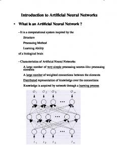
Training curve This is a very useful visual aid to gauging the progress of the learning process. It shows the variation of error E with epoch t:

A smaller value of η gives slower but smoother convergence of E; a larger training rate give a faster but more erratic (ie not reducing E at each epoch) convergence. (Though this last doesn’t -- for this model -- affect the ability of the net to find a solution if one exists, it is good practice to avoid erratic training behaviour as for other neural network models such behaviour is usually damaging.) Perceptron Architectures A variety of network topologies were used in perceptron studies in the 1950s and 1960s. Not all of these were of the simple singlelayer type -- there could be one or more preprocessing layers, usually randomly connected to the input grid, though the perceptron learning algorithm was only able to adapt the weights of the neurons in the output layer, the neurons in the added preprocessing layers having their weights as well as their connections chosen randomly. These extra layers were added because it was observed that quite frequently a single-layer net just couldn’t learn to solve a problem, even after many thousands of epochs had elapsed, but that adding a randomly connected 'hidden' layer sometimes allowed a solution to be found.

24

2-layer perceptron character classifier However it wasn’t fully appreciated that • It was the restriction to a single learning layer (it’s being impossible to use the Widrow-Hoff rule on any but output layer neurons, as it’s only for these neurons that target values are defined) that was the fundamental reason for the failures. • The trial-and-error connection of a preprocessing layer, reconnecting if learning still failed, was in effect a primitive form of training for this hidden layer (a random search in connection and weight space). Limitations of perceptrons (Minsky and Papert, 1969) As described above, there were some desired pattern classifications for which the perceptron training algorithm failed to converge to zero error, and Minsky and Papert deduced that these were when the individual neurons were being required to perform functions of a certain mathematical type, known as non-linearly separable functions.

25

This might not have mattered if the proportion of such functions was small, but unfortunately as the number of inputs to a single BDN neuron grows, the proportion of those functions which might be required to be developed by a net with a single learning layer, but are not representable by a BDN neuron, grows extremely fast (or conversely, the number which can be performed, those which are linearly separable) drops equivalently quickly: n Number of Possible functions 1 4 2 16 3 256 4 65,336 5 ~4.3x109 6 ~1.8x1019

Number of linearly separable functions 4 14 104 1,882 94,572 5,028,134

Proportion of linearly separable functions 1 0.88 0.41 0.03 ~2.2x10-5 ~2.8x10-13

It’s not surprising therefore that Rosenblatt’s group frequently encountered difficulties when using their perceptron nets for image recognition problems. However remember they were able to partly overcome these difficulties with a trial-and-error training method involving a 'preprocessing layer.' It’s the use of such an additional layer -- but with weights acquired by something more efficient than random search -- that underpins modern multilayer perceptron nets, which are not subject to the learning restrictions of Rosenblatt’s day.

MULTILAYER PERCEPTRON (MLP) The MLP, usually trained using the method of error backpropagation, was introduced independently in the mid-1980s by a number of workers (Werbos (1974); Parker (1982); Rumelhart and Hinton (1986)) and is still by far the most widely used of all neural network types for practical applications.

26

In this network the BDN’s step function output is 'softened': n

y = f(∑ w jx j )

where f : Rn → [0,1] not into {0,1}

j=0

This modified output function is the key to the MLP weight change rule, which unlike the single-layer perceptron Widrow-Hoff rule can be defined not just for output layer neurons but for all neurons of the net, including those hidden neurons in layers below the output layer, for which it isn’t possible to directly define a target value, but play a vital role in learning to represent functions of the more difficult non-linearly separable type. This output function must for mathematical reasons: • • • •

be continuous be differentiable be non-decreasing have bounded range (normally the interval [0,1])

The most commonly used such function is the sigmoid

f ( x) =

1 1+ e- x

27

The sigmoid is the 'squashing' function that is most often chosen because • its output range [0,1] can be interpreted as a neural firing probability or firing rate, should that in certain applications be required • it has an especially simple derivative

d e- x f′( x ) ≡ ( f ( x )) = = f ( x )( 1 - f(x) ) dx (1 + e - x )2 which is useful as this quantity needs to be calculated often during the error backpropagation training process.

Backpropagation training process for MLPs With a continuous and differentiable output function like the sigmoid above, it is possible to discover how small changes to the weights in the hidden layer(s) affect the behaviour of the units in the output layer, and to update the weights of all neurons so as to improve performance. The error backpropagation process is based on the concept of gradient descent of the error-weight surface. The error-weight surface can be imagined as a highly complex landscape with hills, valleys etc, but with as many dimensions as there are free parameters (weights) in the network. The height of the surface is the error at that point, for that particular set of weight values. Obviously, the objective is to move around on this surface (ie change the weights) so as to reach its overall lowest point, where the error is a minimum. This idea of moving around on the errorweight surface, according to some algorithmic procedure which moves one -- hopefully -- in the direction of lower errors, is intrinsic to the geometrical view of training a neural network.

28

Gradient descent is the process whereby each step of training is chosen so as to take the steepest downhill direction in the (mean squared) error.

Example: 2-layer MLP with 2 inputs (layer 0), 2 hidden neurons (layer 1) and 1 output neuron (layer 2):

29

The weight-change rule for multilayer networks, considering the change to the jth input weight of the ith neuron in layer l, takes the form

Δw lij = ηδli ylj-1 where

yli = output of unit i in layer l

= f (ali ) where f is the sigmoid firing function

ali = activation of unit i in layer l nl-1

= " wlij y l-1 j (calculated the same way as for BDN neurons) j=0

w lij = real-valued weight from unit j in layer (l-1) to unit i in layer l !

δli = error contributed by unit i in layer l to the overall network (root mean squared) error The above rule for multilayer nets is sometimes known as the generalised delta rule because of the formal similarity between it and the Widrow-Hoff delta rule used for the single-layer perceptron. The essential difference, however, is how the error contribution for neuron i, δli , is now calculated. It can be proved using the principle of gradient descent that the forms this takes for the output layer (layer l=L) and hidden layer (layers l