Under consideration for publication in J. Fluid Mech.
1
Edge states as mediators of bypass transition in boundary-layer flows T. K H A P K O1,2 , T. K R E I L O S3 , P. S C H L A T T E R1,2 †, Y. D U G U E T4 , B. E C K H A R D T5,6 A N D D. S. H E N N I N G S O N1,2 1
Linn´e FLOW Centre, KTH Mechanics, Royal Institute of Technology, SE-100 44 Stockholm, Sweden 2 Swedish e-Science Research Centre (SeRC), Sweden 3 ´ Emergent Complexity in Physical Systems Laboratory (ECPS), Ecole Polytechnique F´ed´erale de Lausanne, CH-1015 Lausanne, Switzerland 4 LIMSI, CNRS, Universit´e Paris-Saclay, F-91405 Orsay, France 5 Fachbereich Physik, Philipps-Universit¨ at Marburg, D-35032 Marburg, Germany 6 J.M. Burgerscentrum, Delft University of Technology, NL-2628 CD Delft, The Netherlands (Received 29 April 2016)
The concept of edge state is investigated in the asymptotic suction boundary layer in relation with the receptivity process to noisy perturbations and the nucleation of turbulent spots. Edge tracking is first performed numerically, without imposing any discrete symmetry, in a large computational domain allowing for full spatial localisation of the perturbation velocity. The edge state is a three-dimensional localised structure recurrently characterised by a single low-speed streak that experiences erratic bursts and planar shifts. This recurrent streaky structure is then compared with predecessors of individual spot nucleation events, triggered by non-localised initial noise. The present results suggest a nonlinear picture, rooted in dynamical systems theory, of the nucleation process of turbulent spots in boundary-layer flows, in which the localised edge state play the role of state-space mediator.
1. Introduction Bypass transition to turbulence in boundary-layer flows is known to proceed via the appearance of localised turbulent spots on a background of streamwise streaks (Kendall 1998; Matsubara & Alfredsson 2001; Brandt et al. 2004; Zaki & Durbin 2005). These spots expand aggressively and fill the plate with turbulent motion further downstream (Emmons 1951). Bypass transition is usually described as a two-step process (Saric et al. 2002). During the receptivity phase, ambient perturbations (e.g. free-stream turbulence or delocalised noise) enter the boundary layer and are converted into streamwise streaks, while in the second phase these streaks become unstable and break down to form turbulent spots. The receptivity phase is usually associated with linear mechanisms, while the secondary instability has traditionally been investigated by linearising around a saturated streaky base flow (Andersson et al. 2001). On a fundamental level, this picture of transition is not entirely satisfying because i) it is essentially based on disconnected linear steps, ii) streaks do not form a regular pattern and their stability must be investigated case by case, and iii) secondary stability analysis uses spatially extended modes and therefore fails at explaining the localised nature of the ensuing spots. Despite years † Email address for correspondence:
[email protected]
2
T. Khapko et al.
Wu
Ws
Figure 1. Sketch of the state space. The basin boundary coincides with the stable manifold W s of the edge state; W u is its unstable manifold and points either towards the laminar state or to the turbulent attractor. The minimal seed is the point on the edge closest to the laminar state in energy norm.
of efforts to understand the nucleation of a turbulent spot using secondary instability concepts, there has been no accepted consensus to distinguish the perturbations leading to turbulence from those experiencing viscous decay. In wall-bounded flows such as plane Couette or Poiseuille flows, turbulent structures can also emerge from localised disturbances, even when the laminar base flow is linearly stable. This has lead recently to the abstract nonlinear concept of laminar–turbulent boundary in state space. According to this picture, a manifold of co-dimension one separates initial perturbations that rapidly decay from those experiencing turbulent evolution (Itano & Toh 2001; Skufca et al. 2006; Schneider et al. 2007). This picture carries over to extended systems, in which the edge state, i.e. the relative attractor on this separating manifold, displays robust spatial localisation (Mellibovsky et al. 2009; Willis & Kerswell 2009; Duguet et al. 2009; Schneider et al. 2010; Zammert & Eckhardt 2014). The perturbation energy of such edge states is notoriously low, but not as low as the minimal seed considered in recent studies, itself also a point on the laminar–turbulent boundary (Duguet et al. 2013; Kerswell et al. 2014). Independently of its temporal dynamics (steady, periodic or even chaotic), the edge state represents a saddle in the global state space of the system (see figure 1). Trajectories initiated arbitrarily close to its stable manifold W s approach the neighbourhood of the edge state for a short time, before being flung away along its unstable manifold W u . Non-localised initial perturbations are no exception (Duguet et al. 2010b; Schneider et al. 2010). As a consequence, even initial noise with a carefully selected amplitude evolves into a localised seed that later spreads like a turbulent spot. It is noteworthy that also finite-amplitude noise (with a less constraint amplitude) dissipates and leaves a streaky background from which isolated turbulent spots emerge (see e.g. Duguet et al. (2010a) in plane Couette flow). The visual resemblance between localised edge states and incipient turbulent spots has also been noted, but never quantified. This leads to the following questions: can the spot nucleation process be described efficiently using this geometric state space picture involving the edge state? How far can this concept also be extended to realistic bypass transition in boundary layer flows? Edge states have also recently been identified in linearly stable boundary-layer flows, by considering localised initial disturbances to the laminar base flow, and varying their amplitude, until the dynamics reaches an unstable equilibrium regime, characterised by robust spatial localisation (Cherubini et al. 2011; Duguet et al. 2012). Spatially developing boundary layers, despite their ubiquitous importance in nature and industry, are
Edge states as mediators of bypass transition in boundary-layer flows
3
only poorly adapted to edge-state computations, because the slow spatial growth complicates the search for an asymptotically defined flow regime. The asymptotic boundary layer (ASBL) is another boundary-layer flow, where suction at the wall equilibrates the growth of the boundary layer. The laminar flow solution, as well as the corresponding turbulent mean profile, are hence streamwise- and time-independent. The ASBL appears better suited to long-time edge state computations, because it can be simulated using periodic boundary conditions (Kreilos et al. 2013; Khapko et al. 2013, 2014). The present investigation consists of two parts. In the first part, the edge state of ASBL is computed in a numerical domain sufficiently large to allow for three-dimensional localisation. Its chaotic dynamics is investigated and compared with former computations in more constrained geometries. In a second part, a set of numerical simulations of ASBL are analysed, initiated using different realisations of random noise. The current emphasis is on identifying the signature of the edge state during spot nucleation. In an effort to match realistic operating conditions, no special discrete symmetry has been imposed in the computations, and the amplitude of the initial noise in the second part has been chosen arbitrarily (no bisection performed). The results successfully confirm that localised edge states act as state space mediators during the process of spot nucleation.
2. Flow case and numerical methodology An asymptotic suction boundary layer forms when fluid flows above a porous flat plate subject to constant uniform suction (Griffith & Meredith 1936). Suction balances the natural spatial growth of the boundary layer, eventually leading to a streamwise-independent flow. The laminar flow solution reads u(y) = U∞ (1 − e−yVS /ν ), v = −VS , with u and v the streamwise and wall-normal velocity components, y the distance from the wall, U∞ the free-stream velocity and ν the kinematic viscosity of the fluid. It is realisable in experiments (Antonia et al. 1988; Fransson & Alfredsson 2003). The streamwise and spanwise coordinates are denoted x and z. The Reynolds number is defined classically as the ratio Re = U∞ /VS , with VS > 0 the suction velocity. Non-dimensionalisation is based on U∞ and on the displacement thickness δ ∗ = ν/VS . From this point onwards, all quantities are non-dimensional. The flow is linearly stable up to Re ≈ 54370 (Hocking 1975) but finite-amplitude perturbations can sustain turbulence for Re ≥ 270 (Khapko et al. 2016). Temporal simulations are performed using the spectral code SIMSON (Chevalier et al. 2007). The edge state is tracked iteratively using the standard bisection procedure of Skufca et al. (2006). A new bisection is started once the separation between the two last diverging trajectories of a previous bisection exceeds in norm a predefined threshold. Following Khapko et al. (2013, 2014), edge computations have been performed at Re = 500 where turbulence is an attractor. Two numerical domains D1 and D2 have been considered, respectively, for edge tracking and noise-induced transition: D1 has dimensions [Lx , Ly , Lz ] = [800, 15, 100] with spectral resolution (Nx , Ny , Nz ) = (2048, 121, 384), whereas D2 has [Lx , Ly , Lz ] = [300, 20, 150] with (Nx , Ny , Nz ) = (384, 97, 384). The large dimensions of D1 ensure full spatial localisation of the edge state while the choice for D2 results from a trade-off between capturing localisation and restricting the transition to single nucleation events. Resolution requirements for edge tracking have already been assessed in smaller numerical domains (Khapko et al. 2013). The slightly lower resolution used in D2 improves nucleation statistics without affecting the initial stages of transition.
4
T. Khapko et al.
Figure 2. Three-dimensional snapshot of the edge state (t = 2.1 × 10⁴ , see square in figure 4a). Low- (blue) and high-speed (red) streaks shown with isosurfaces of the streamwise velocity fluctuations u0 = ±0.05, and vortices with λ2 = −2 × 10⁻⁴ isosurfaces (green). Flow from left to right. The whole computational domain is shown. Supplementary movie is available in the Supplementary Material.
〈|v′|〉x(z,y=1)
10 10 10 10
−2 (b) 10
−3
−3
10
−4
−4
−5
10
−5
10
z
10
−2
〈|v′|〉 (x,y=1)
(a) 10
−6
−7
−7
10
−8
10 −50
−6
10
−8
−25
0
25
z
50
10 −400
−200
0
200
400
x
Figure 3. Wall-normal fluctuations v 0 (y = 1) averaged in the streamwise (a) or spanwise direction (b). Instantaneous (grey) vs. time-averaged (black) profiles.
3. Localised edge state Edge tracking results asymptotically in a fully localised structure. A three-dimensional snapshot of the edge state is shown in figure 2. It consists of a few low- and highspeed streaks and streamwise vortices located mostly along one main low-speed streak. The structure resembles a turbulent spot in its early development stage, except that it neither decays nor grows in size. For slightly higher initial amplitudes, the same flow structure quickly breaks down into turbulence that spreads throughout the whole domain. Importantly, this edge state is localised in the three spatial dimensions. In the wallnormal direction it is contained within the boundary layer. Full localisation in the wallparallel directions is demonstrated in figure 3 by considering the norm of the wall-normal fluctuations |v 0 | at y = 1. The averages of |v 0 | in the x or z direction, denoted with h·i, are then computed to assess the spanwise and streamwise localisation (see figure 3). The drop in magnitude in z by four decades is consistent with an exponential decay, whereas the decay by two decades in x is compatible both with exponential or power-law decay (Zammert & Eckhardt 2014). The temporal dynamics of the edge state is monitored in figure 4(a) using the cross-flow energy Z Ecf (t) = (v 02 + w02 ) dx dy dz ≡ Ev + Ew , (3.1) Ω
based on the wall-normal and spanwise velocity fluctuations. This quantity leaves aside the fluctuations associated with the streamwise streaks, characterised by weak decay
Edge states as mediators of bypass transition in boundary-layer flows
2.5
2.5
2
2
t / 104
(b) 3
t / 104
(a) 3
1.5
1.5
1
1
8
6
4
2
0
−40
−20
Ecf
0
20
5
40
z −0.2
−0.1
0
0.1
0.2
Figure 4. (a) Cross-flow energy Ecf (t). Open circles (resp. crosses) correspond to maxima (resp. minima) of Ecf . The snapshot in figure 2 is marked with a square, those from figure 5 with blue crosses. (b) Space–time (z, t) diagram of hu0 ix (y = 1). Averaging in x is performed here locally in a neighbourhood around the active core of the state.
rates. Variations of Ecf remain chaotic but display a clear alternation of calm phases with bursting phases. The spatio-temporal dynamics of the streaks is relatively simple once displayed in a space–time diagram as in figure 4(b). The quantity visualised here is the streamwise velocity fluctuation u0 (y = 1) averaged locally over 50 streamwise units. When Ecf is low, only one low-speed streak remains active, which defines the recurrent ‘active core’ of the edge state. The active low-speed streak is flanked by staggered streamwise vortices. A sinuous mode develops and ultimately breaks down the streak (see left column in figure 5), in association with a burst of Ecf in figure 4(a). In the breakdown process new vortices are created around the active region, regenerating new streaks. One of them takes the role of the active core and the cycle is closed modulo a spanwise shift. This is confirmed in figure 4(b) which shows erratic shifts in z over periods of ≈ 103 − 104 time units. The whole regeneration cycle is the localised counterpart of the dynamics described in shorter numerical domains of ASBL (Kreilos et al. 2013; Khapko et al. 2013, 2014), and bears many similarities with the self-sustaining cycle of near-wall turbulence (Hamilton et al. 1995). The fluctuations reaching higher up in the boundary layer are shed downstream from the active core, where the shear is not strong enough to sustain them. This mechanism, also reported in spatially developing boundary layers (Duguet et al. 2012), maintains the x-localisation of the edge state.
4. Nucleation process Sinuous modes growing on low-speed streaks have often been reported in experiments and computations of bypass transition (Brandt et al. 2004; Yoshioka et al. 2004). Varicose modes of instability have also been predicted and observed in boundary layer flows
6
T. Khapko et al.
Figure 5. Comparison of the edge state during calm phases (t = 12700, 15400) and pre-nucleation events in noise-induced transition. Visualisation similar to figure 2, but with different isovalues (u0 = ±0.13 and λ2 = −4 × 10⁻⁴ ). Only parts of the computational domains D1 and D2 (approximately 140 × 40) are shown. Flow from left to right.
Characteristic
edge state in calm phase pre-nucleation events
streak width [δ ∗ ]
3.46 ± 0.52
3.75 ± 0.63
streak intensity [U∞ ]
0.25 ± 0.03
−0.25 ± 0.04
33 ± 10
27.5 ± 6
instability wavelength [δ ∗ ]
Table 1. Quantitative comparison of edge state and noise-induced pre-nucleation events.
but are outweighed statistically by the sinuous ones (Schlatter et al. 2008). The visual similarities between the edge-state dynamics and pre-nucleation episodes in bypass transition suggest that the emergence of streaks may be regarded as the approach to W s , the stable manifold of the edge state. A crucial difference lies in the treatment of the sinuous modes, traditionally interpreted as a growing departure from a streaky non-sinuous base flow. The current sinuous oscillations are inherently part of the dynamics of the edge state. Constraining the dynamics to remain on W s on the one hand leads to break-up and later reformation of exactly one active streak. Unconstrained computations on the other hand do not lead to one active streak reforming after breakdown: either the streak does not reform and the flow relaminarises, or several low-speed streaks emerge which cascade into turbulent motion and finally lead to an aggressively expanding turbulent spot. Both scenarios take the flow away from the edge state, which is consistent with a state space escape along either direction of W u . In order to test this hypothesis, we consider a series of simulations of transition ASBL at Re = 500 with non-localised noise as an initial condition, and investigate whether the edge state can be, even transiently, identified in these simulations. The noise consists of a random superposition of Stokes modes spanning the whole domain with length scale on the order of 10 (Chevalier et al. 2007). The magnitude for the noise amplitude is chosen to ensure transition through nucleation and growth of turbulent spots, but it is not optimised to result in trajectories that spend a long time near the edge (as could be done using edge tracking) since we did not want to artificially force visits to the edge states. As noted in section 2, the numerical domain D2 is chosen sufficiently large for localised spots to emerge, but still small enough so that typically only one or two distinct localised spot events are observed. We begin with a qualitative comparison in figure 5 between well-chosen snapshots on
Edge states as mediators of bypass transition in boundary-layer flows (a)
7
(b) 20
2.2 2
15 w
1.6
√E
√Ew
1.8
1.4
10
1.2 5 1 0.8 0.5
1
1.5
√Ev
2
0 0
2
4
6
8
10
√Ev
√ √ Figure 6. State space projection on Ev and Ew . (a) Projection of the chaotic edge state. Circles and crosses indicate extrema of Ecf as in figure 4(a). (b) Transition from four different noise amplitudes (green, magenta, shades of grey and blue colours in the plot), with most of the trajectories corresponding to one of the noise levels (grey). Noisy initial conditions with crosses, edge state in red. Supplementary movie is available in the Supplementary Material.
the edge trajectory and local precursors of turbulent spots. Both instances involve one low-speed streak with sinuous instabilities with similar size and magnitude. More quantitative evidence that the edge state is actually embedded in the noise simulations is based on three-dimensional measurements (statistics are based on 13 instances corresponding to all local minima of Ecf ). We report in the two set-ups the spanwise width of the most intense low-speed streak, its intensity (deviation from the laminar flow) and the streamwise wavelength of the growing sinuous instability. The quantitative similarity between the statistical averages reported in table 1 is remarkable. Further quantitative evidence that noise-initiated trajectories do visit the neighbourhood of the edge state comes from energetic √ √ projections of the state space. In figure 6, the dynamics is projected on the ( Ev , Ew ) plane. In this projection, the chaotic edge state is a convoluted object residing in a small bounded region of the state space (see figure 6a). Trajectories with the lowest levels of initial noise (green line in figure 6b) continue towards the laminar state while the flow slowly laminarises, suggesting that the corresponding initial conditions are within the basin of attraction of the laminar state. For most initial conditions with higher amplitude, apparent approaches to the edge state in figure 6(b) are followed by an abrupt increase in energy: the corresponding initial conditions belong to the basin of attraction of the turbulent state. The cloud of initial conditions is hence staggered along W s . Several simultaneous nucleations result in higher energies and, thus, in a larger distance to the edge in figure 6(b). Therefore, the distance of the closest approach is smallest for the trajectories involving one single nucleation event. Once the spots appear, they grow in size, invading the domain, with the energy steadily growing in figure 6(b). In the current finite-size system the energy saturates when the entire volume has become turbulent. Since the latter is domain-dependent, we choose not to show it in figure 6(b). The geometric structure emerging from figure 6(b) is then directly comparable with figure 1. All trajectories in figure 6(b), despite starting from different parts of the state space (the variability of Ecf (t = 0) is here approximately 70%), approach the location of the edge state and leave together along a single direction. This is consistent with an approach along W s (characterised by a very large effective dimension) and an escape along the one-dimensional W u . The time it takes to nucleate a turbulent spot starting from noise is different for each individual state space trajectory. This nucleation time tn is defined as the time at which a predefined threshold in Ecf = 70 is reached. A histogram of tn for different trajectories
8
T. Khapko et al. 7
40
(a)
(b)
5 20
d
number of events
6 30
4 10 3 0
400
600
800 1000 1200 1400 1600 1800
tn
2
400
600
800 1000 1200 1400 1600 1800
tn
Figure 7. (a) Distribution of the nucleation events in time obtained for the same initial noise level. (b) Nucleation time tn vs. the distance of the closest approach to the edge d.
starting from the same noise level is shown in figure 7(a). Its exact shape depends on the statistical distribution of initial conditions and details of the dynamics. However, we infer from the data in figure 6(b) that closer approaches to the edge state lead to delayed transition. This is verified in figure 7(b) by plotting for each noise realisation the measured nucleation √ time √ versus the associated minimal distance to the calm phase on the edge in the ( Ev , Ew ) plane. The trend is clear and, despite the nonlinear context, fully consistent with the linear approach to a saddle point: the closer a trajectory comes to the edge state, the longer the time it spends in its vicinity, hence the later it reaches the turbulent attractor. This behaviour, expected in the direct (linearised) neighbourhood of a saddle point, is confirmed here at a finite distance from the saddle. Note that in an experimental set-up, a distribution of nucleation times translates into a distribution of nucleation positions because of the mean advection.
5. Discussion and conclusions Computation of the edge state in ASBL in an extended numerical domain has lead to a flow state localised in the three spatial directions. Its dynamics is chaotic in time and involves recurrent visits to an active core consisting of one low-speed streak developing sinuous instabilities. The regeneration mechanism identified is strongly reminiscent of similar computations in constrained numerical domains (Kreilos et al. 2013; Khapko et al. 2013), and appears thus generic for ASBL. Besides, localised recurrent low-speed streaks subject to sinuous instabilities have also been reported as edge states in spatially developing boundary layer (Duguet et al. 2012) with imposed spanwise symmetry, suggesting possible direct extensions to a wider class of boundary layer flows. The classical description of a nucleation event leading to a turbulent spot is based on the linear instability of some well-chosen streak state selected by the receptivity process. This can here be reformulated within a more global state space picture where the central mediator is the edge state along with his stable and unstable manifolds W s and W u . The approach along W s incorporates both the classical receptivity stage and also the emerging localisation, while the escape along W u captures all the mechanisms, formerly described by secondary instability concepts, now in a localised context. The concept of escape from the edge was used recently to model the nucleation process (Kreilos et al. 2016), without taking into account the receptivity phase encoded in the approach to W s . The present study demonstrates that this picture does not only hold for very carefully
Edge states as mediators of bypass transition in boundary-layer flows
9
selected initial conditions designed to lie on W s , but that it is robust enough for a much wider class of perturbations. Careful unbiased analysis of a set of simulations initiated by non-localised noise convincingly demonstrates that a robust coherent structure, quantitatively analogous to the recurrent streak state on the edge, is also closely visited after the initial phase where the noise dissipates. Former evidence for the presence of a well-defined finite-amplitude streaky state as precursor to spot nucleation appeared in various shear flows studies, for trajectories starting either from a minimal seed (Duguet et al. 2013) or from free-stream turbulence (Schlatter et al. 2008). A finer representation of the state space geometry with a proper metrics, taking into account the chaotic behaviour on the edge, its expanding Lyapunov directions and the translational invariance of the system, would improve our representation of the system and the measure of how close the edge state is approached. The minimal seed is another well-defined point in this geometry, also connected to the edge state, and its dynamic role in a realistic transitional flow also deserves further study. This view on the bypass-transition process appears now generic to most wall-bounded shear flows, where transition can be considered as an initial value problem in a temporal set-up. The main challenge is to reconcile such a set-up with permanent excitations fluctuating both in time and space. The extension of an abstract state-space description to spatially developing boundary layer flows still faces further open questions. While the concept of localised edge state is useful to describe the formation of one individual turbulent spot, the case of truly extended systems (i.e. larger than the typical correlation distance) demands a paradigm shift: as multiple simultaneous nucleation events occur at remote (ideally uncorrelated) locations on the plate, the description of the system in terms of a unique dynamical system reaches its limits. The price to pay is to trade the deterministic picture for a statistical description of the nucleation process involving the definition of a probabilistic nucleation rate. We acknowledge that the results of this research have been achieved using the PRACE3IP project (FP7 RI-312763) resource ARCHER based in UK at EPCC. Some additional runs were performed using the resources provided by SNIC (Swedish National Infrastructure for Computing).
REFERENCES Andersson, P., Brandt, L., Bottaro, A. & Henningson, D. S. 2001 On the breakdown of boundary layer streaks. J. Fluid Mech. 428, 29–60. Antonia, R. A., Fulachier, L., Krishnamoorthy, L. V., Benabid, T. & Anselmet, F. 1988 Influence of wall suction on the organized motion in a turbulent boundary layer. J. Fluid Mech. 190, 217–240. Brandt, L., Schlatter, P. & Henningson, D. S. 2004 Transition in boundary layers subject to free-stream turbulence. J. Fluid Mech. 517, 167–198. Cherubini, S., De Palma, P., Robinet, J. C. & Bottaro, A. 2011 Edge states in a boundary layer. Phys. Fluids 23, 051705. Chevalier, M., Schlatter, P., Lundbladh, A. & Henningson, D. S. 2007 A pseudospectral solver for incompressible boundary layer flows. Tech. Rep. TRITA-MEK 2007:07. KTH Mechanics, Stockholm, Sweden. Duguet, Y., Monokrousos, A., Brandt, L. & Henningson, D. S. 2013 Minimal transition thresholds in plane Couette flow. Phys. Fluids 25, 084103. Duguet, Y., Schlatter, P. & Henningson, D. S. 2009 Localized edge states in plane Couette flow. Phys. Fluids 21, 111701. Duguet, Y., Schlatter, P. & Henningson, D. S. 2010a Formation of turbulent patterns near the onset of transition in plane Couette flow. J. Fluid Mech. 650, 119–129.
10
T. Khapko et al.
Duguet, Y., Schlatter, P., Henningson, D. S. & Eckhardt, B. 2012 Self-sustained localized structures in a boundary-layer flow. Phys. Rev. Lett. 108, 044501. Duguet, Y., Willis, A. P. & Kerswell, R. R. 2010b Slug genesis in cylindrical pipe flow. J. Fluid Mech. 663, 180–208. Emmons, H. W. 1951 The laminar-turbulent transition in a boundary layer - Part I. J. Aero. Sci. 18 (7), 490–498. Fransson, J. H. M. & Alfredsson, P. H. 2003 On the disturbance growth in an asymptotic suction boundary layer. J. Fluid Mech. 482, 51–90. Griffith, A. A. & Meredith, F. W. 1936 The possible improvement in aircraft performance due to the use of boundary layer suction. Tech. Rep. 3501. Royal Aircraft Establishment. Hamilton, J. M., Kim, J. & Waleffe, F. 1995 Regeneration mechanisms of near-wall turbulence structures. J. Fluid Mech. 287, 317–348. Hocking, L. M. 1975 Non-linear instability of the asymptotic suction velocity profile. Q. J. Mech. Appl. Math. 28 (3), 341–353. Itano, T. & Toh, S. 2001 The dynamics of bursting process in wall turbulence. J. Phys. Soc. Jpn. 70, 703–716. Kendall, J. M. 1998 Experiments on boundary-layer receptivity to free-stream turbulence. AIAA Paper . 98-0530. Kerswell, R. R., Pringle, C. C. T. & Willis, A. P. 2014 An optimization approach for analysing nonlinear stability with transition to turbulence in fluids as an exemplar. Rep. Prog. Phys. 77, 085901. Khapko, T., Duguet, Y., Kreilos, T., Schlatter, P., Eckhardt, B. & Henningson, D. S. 2014 Complexity of localised coherent structures in a boundary-layer flow. Eur. Phys. J. E 37 (32). Khapko, T., Kreilos, T., Schlatter, P., Duguet, Y., Eckhardt, B. & Henningson, D. S. 2013 Localised edge states in the asymptotic suction boundary layer. J. Fluid Mech. 717, R6. Khapko, T., Schlatter, P., Duguet, Y. & Henningson, D. S. 2016 Turbulence collapse in a suction boundary layer. J. Fluid Mech. 795, 356–379. Kreilos, T., Khapko, T., Schlatter, P., Duguet, Y., Henningson, D. S. & Eckhardt, B. 2016 Bypass transition and spot nucleation in boundary layers. Phys. Rev. Fluids (under review). Kreilos, T., Veble, G., Schneider, T. M. & Eckhardt, B. 2013 Edge states for the turbulence transition in the asymptotic suction boundary layer. J. Fluid Mech. 726, 100–122. Matsubara, M. & Alfredsson, P. H. 2001 Disturbance growth in boundary layers subjected to free-stream turbulence. J. Fluid Mech. 430, 149–168. Mellibovsky, F., Meseguer, A., Schneider, T. M. & Eckhardt, B. 2009 Transition in localized pipe flow turbulence. Phys. Rev. Lett. 103, 054502. Saric, W. S., Reed, H. L. & Kerschen, E. J. 2002 Boundary-layer receptivity to freestream disturbances. Annu. Rev. Fluid Mech. 34, 291–319. Schlatter, P., Brandt, L., De Lange, H. C. & Henningson, D. S. 2008 On streak breakdown in bypass transition. Phys. Fluids 20, 101505. Schneider, T. M., Eckhardt, B. & Yorke, J. A. 2007 Turbulence transition and the edge of chaos in pipe flow. Phys. Rev. Lett. 99, 034502. Schneider, T. M., Marinc, D. & Eckhardt, B. 2010 Localized edge states nucleate turbulence in extended plane Couette cells. J. Fluid Mech. 646, 441–451. Skufca, J. D., Yorke, J. A. & Eckhardt, B. 2006 Edge of chaos in a parallel shear flow. Phys. Rev. Lett. 96, 174101. Willis, A. P. & Kerswell, R. R. 2009 Turbulent dynamics of pipe flow captured in a reduced model: puff relaminarization and localized ‘edge’ states. J. Fluid Mech. 619, 213–233. Yoshioka, S., Fransson, J. H. M. & Alfredsson, P. H. 2004 Free stream turbulence induced disturbances in boundary layers with wall suction. Phys. Fluids 16 (10), 3530–3539. Zaki, T. A. & Durbin, P. A. 2005 Mode interaction and the bypass route to transition. J. Fluid Mech. 531, 85–111. Zammert, S. & Eckhardt, B. 2014 Streamwise and doubly-localised periodic orbits in plane Poiseuille flow. J. Fluid Mech. 761, 348–359.