Edge Tracking of Textured Objects with a Recursive Particle Filter

Edge Tracking of Textured Objects with a Recursive Particle Filter Thomas M¨orwald∗ Vienna University of Technology

Michael Zillich† Vienna University of Technology

Abstract This paper proposes a new approach of model-based 3D object tracking in real-time. The developed algorithm uses edges as features to track, which are easy and robust to detect. It exploits the functionality of modern highly parallel graphics boards by performing hidden face removal, image processing, texturing and particle filtering. Using a standard 3D -model the tracker requires neither memory and time -consuming training nor other pre-calculations. In contrast to other approaches this tracker also works on objects where geometry edges are barely visible because of low contrast. Keywords: Object tracking, edge detection, 3D tracking, realtime, image processing, feature matching Best to read in color.

1

Introduction

Markus Vincze‡ Vienna University of Technology

[Lucie Masson and Jurie 2004] also uses edges and textures for tracking. They extract point features from the texture and use them together with the edges to calculate the pose. This turns out to perform very fast and robust against occlusion. Our approach not only uses patches but the whole texture, which usually lets the pose converge very quickly to the accurate pose. Since the algorithm runs on the GPU, it is as fast as the method in [Lucie Masson and Jurie 2004]. The work presented in [M. Vincze and Zillich 2001] uses edge features to track but does not take into account texture information. This makes it less robust against occlusion. Since the search area in that approach is very small, it is also less robust against fast movement and getting caught in local minima. The work presented in this paper is based on [Klein and Murray 2006] where they take advantage of graphics processing by projecting a wireframe model into the camera image. Then a particle filter with a Gaussian noise model is used to evaluate the confidence level with respect to the pose.

Tracking the pose of a three dimensional object from a single camera is a well known task in computer vision. What seems to be simple for humans turns out to be significantly more complicated for computers. While humans are able to perform highly parallel image processing, even modern central processing units (CPUs) have problems calculating the pose of an object with sufficient accuracy, robustness and speed. This leads to the idea of using modern graphics cards, which also work in parallel, to solve this problem. This approach exploits the parallel power of graphics processing units (GPUs) by comparing edge features of camera images and a 3D -model. Graphics boards are designed to render virtual scenes as realistically as possible. The main idea is to compare those virtual scenes with an image captured from reality. Texturing is a common method of simulating realistic surfaces. In this paper, the edges of those textures are used for comparison. Fast progress in computer science will soon allow the inclusion of more and more optical effects like shadows, reflections, shading, occlusions or even smoke, fire, water or fog.

1.1

Related work

One of the first successful approaches of tracking objects by their edges was RAPiD [Harris 1992]. It uses points on edges and searches for correspondence to its surroundings along the edge gradient. However this method lacks robustness and several improvements were applied to overcome this problem as in [Drummond and Cipolla 1999; Philipp Michel 2008; Luca Vacchetti and Fua 2004; Klein and Drummond 2003]. Another approach is to globally match model primitives with those from the camera image [Lowe 1992; Gennery 1992; D. Koller and Nagel 1993; Kosaka and Nakazawa 1995; A. Ruf and Nagel 1997]. This method has been used for robot and car tracking applications, but was later replaced by improved versions based on RAPiD. ∗ e-mail:

[email protected] [email protected] ‡ e-mail: [email protected] † e-mail:

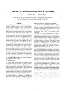
Figure 1: Edges from geometry vs. edges from texture Our approach not only uses geometry edges but also edge features from textures which extends the class of trackable models by those that have curved surfaces as illustrated on the right of Figure 1. This is because in a standard 3D -model curvature is approximated by triangles and quadrangles which would produce virtual edges which do not correspond to the actual edges as shown on the left of Figure 1. The particle filter is extended by using it in a recursive design that evaluates a single pose estimate given by the most likely particles.

1.2

Overview

The idea of this approach is to • extract the edges from the incoming camera image, • extract the edges from the textured 3D -model, • generate hundreds of slightly different views of the model relative to a pose estimate, • calculate the most likely pose of the model by matching the edges of the camera image and the 3D -model. The algorithm developed is separated into two parts. The preprocessing in Section 2, where all possible pre-calculations are made

and the recursive particle filtering in Section 3, which generates several hundred poses and for each of them evaluates the confidence level. Therefore the second part is very time -crucial. A linear Kalman filter described in Section 4 is applied for smoothing the resulting trajectory. Section 5 gives some hints on how to implement the proposed methods. The results in Section 6 and the conclusion in Section 7 summarize the advantages and strengths of the presented tracker.

2

Preprocessing

e In the preprocessing stage of the algorithm the edge image IC of the incoming camera image IC is extracted and stored for comparison later. The color surface S of the object to track is projected into the incoming image IC and the edges are calculated again. This edge image of the object ISe is then used to re-project to the geometry in world space which results in the corresponding edge map of the original surface S e .

forward projection

edge detection ISe

Forward projection

The 3D -model is projected into the camera image IC as defined by Equation (2). Using the camera image IC takes into account that edges are not visible when there are similar light and color conditions in the background. Then the edges of the image are extracted using Equation (1). The transformation of the model from world space to image space is performed by the following matrix operations: uS

=

IS (u, v)

=

Tp XvS  S(vS ) IC (u, v)

(2) if (u, v) ∈ U else

where IS is the camera image with the projected model. U defines the geometry of the object in image space with uS = [uS , vS ] ∈ U Tp denotes the projection- and X the model view or world transformation matrix which defines the pose of an object to track with a rotational and translational term R and t. » – R t X= 0 1

S,X

IS

2.2

IC

The geometry of the object in world space V is represented by its vectors vS = [xS , yS , zS ] ∈ V

edge detection

v projection

e IC

edge detection

re-projection Se

v

u

Figure 2: Flow chart of preprocessing

2.1

Edge detection

The edges I e are found by convolving the original image I with a Gaussian smoothing G and the two Sobel kernels Hs,x and Hs,y as described in [Burger and Burge 2008]. „ e « „ « Ix Hx ∗ G ∗ I Ie = (1) = e Iy Hy ∗ G ∗ I Furthermore, the result is improved by applying thinning and spreading algorithms. Note that for the gradient calculation in Section 3.2 the x and y values are stored separately. Figure 3 shows the different results of edge detection where the xand y-components of the gradient are stored in the red and green color channel. The detection tolerance can be influenced by applying spreading, which broadens the edges by a specific number of pixels according to the tolerance level. This means that instead of searching for edge pixels close to each other, the line width of the edge is raised as shown in Figure 3, which broadens the matching area.

re-projection u Figure 4: Forward projection and re-projection

2.3

Re-projection

The idea of re-projection is to replace the color surface of the 3D model with the corresponding edge map. Note that it is not possible to do the image processing on the color surface S of the object directly, as the edge features get distorted and thinned out when they are projected to image space and therefore wrongly fail the edge matching test. Comparing the edges of the model with the camera image requires the same methods applied to the same point of view and also the same scaling of the edge width. Using a particle filter requires drawing the model several hundred times at different poses Xi with i = 1...N . Replacing the surface

Figure 3: Edge detection results from left to right: original, no spreading, one time spreading, three times spreading

and running the edge detection algorithm for each particle would cause the tracker to be far away from real-time capability. For this reason, the surface of all particles is replaced by only one edge map ISe , calculated by using the prior tracking result X+ . This, in principle causes the same problems as mentioned above, but assuming that the motion of the particles Xi remains small within one tracking pass, the distortions and thinning out can be disregarded.

3

ISe particle generation

Recursive particle filtering

ISe i

The reason for this setup is to benefit from the robustness and speed of a particle filter. For higher accuracy, the standard deviation of the noise is reduced in each recursion. The linear Kalman filter is attached just for fine tuning as mentioned above.

3.1

X+ , fc , wm

For each tracking pass the recursive particle filtering executes the methods shown in Figure 5. First the particles i = [1 . . . N ], representing the pose of the object, are generated using Gaussian noise. Then the confidence level of each particle i is evaluated by matche ing it against the edge image of the camera IC . If there is still processing time tf remaining, then a further recursion step of particle generation and evaluation of the confidence levels is performed with different parameters as described in Section 3.4. Otherwise the maximum likely particle is passed to the next step. The linear Kalman filter, including a physical motion model, is attached to the outcome of the recursive particle filter to fine tune the result and remove remaining jitter. As this additional filter is not part of the recursion it is explained in Section 4.

e IC

confidence evaluation X+ if(tf < t30Hz ) X+ Kalman filter ¯+ X best match

Figure 5: Block scheme of motion with recursive particle filter and Kalman filter

Particle generation

The prior pose X− i of each particle is calculated by perturbing the posterior X+ with Gaussian noise n(σ 2 ) with a standard deviation scaled by the prior confidence level of the pose wm , a scaling factor for motion effect fm and a scaling factor fc set by each recursion step: X− i i

= =

X+ + n(σ 2 (wm , fm , fc )) [1 . . . N ]

(3)

The standard deviation is evaluated by σ = σ I fm fc .(1 − wm )

(4)

where the confidence level of the prior pose wm is multiplied to the initial standard deviation σ I so that the particle distribution narrows with higher confidence. The motion effect fm takes into account that motion in world space along the camera viewing axis causes less change in image space then the same motion orthogonally to the viewing axis. fc becomes smaller with each recursion step in the particle filter. σ I is implemented as a parameter to be set by the user, but should be evaluated automatically in the future regarding the tracking conditions.

3.2

Confidence level

Each particle is tested against the camera image and a confidence level is calculated. Therefore the correlation between the gradients of the edges gSi (u, v) and gC (u, v) is evaluated by comparing the direction of the edges at each image point (u, v). „ e « ISi ,x (u, v) gSi (u, v) = e ISi ,y (u, v) « „ e IC,x (u, v) gC (u, v) = e IC,y (u, v) The angles between those vectors are calculated, producing the edge correlation image Φi : φ

=

Φi (u, v)

=

arccos (gSi .gC ) 8 if < 1 − 2φ π if 1 − 2|φ−π| π : 0 if

φ < π/2 φ > π/2 (u, v) ∈ / vS′

(5)

Note that it is assumed that the result of the arccos() function lies within 0 and π. The image Φi now contains the degree of correlation between the pose suggested by the particle i and the camera

image. The angular deviation of the edge angles Φi is scaled to the range of 0 to 1. The confidence level wi is evaluated as follows: „ « mi 1 mi wi = + ni nmax W

(6)

with mi ni W

= = =

Z Z

∝

wm =

M 1 X wk M k=1

Experiments have shown that increasing the number of most likely particles M to consider in the mean confidence, while lowering the standard deviation in Equation (4) by fc and the edge width (see Figure 3) for each further recursion obtains good results.

Φi (u, v)dvdu

Zu Zv

3.4 |ISe i (u, v)|dvdu

u

v

N X

wi

i=1

nmax

with

max(ni )

The first term within the brackets is the percentage of matching edge pixels mi with respect to the total visible edge pixels ni . Calculating the confidence level only with this term would cause the tracker to lock when only one side of the 3D object is visible. When at this special pose the object is rotated slightely, another side of the object becomes visible. The particle matching this rotation would be equal or most often less then the prior front facing particle. The reason for this is that the number of matching pixels mi grow less than the total visible pixels ni when rotating the object out of the front side view. This effect amplifies when taking into account that edge detection for strongly tilted faces is very faulty.

Recursion

The methods described in Section 3.1 and 3.2 are performed for each of the hundreds of particles. The idea of recursion is to take advantage of the information gain when calculating. This means that the N particles are divided into subranges R1 , R2 , R3 , . . . and so forth. For every range Rk , the pose estimate X+ and confidence level wm of the previous particle filtering Rk−1 is used. The standard deviation for the particle generation is reduced by the scaling factor fc , which narrows the search area of the filter. Therefore Equation (3) becomes ` ´ X− = X+ (Rk−1 ) + n σ 2 i (Rk ) i = [1 . . . Nk ] with σ = σ I fm fc (Rk−1 ).(1 − wm (Rk−1 ))

The second term allocates more weight to the total number of matching pixels mi which is intrinsically higher for the rotated particle. nmax which are the maximum visible edge pixels in the actual area scales the pixels to the proper range. As this summation would lead to confidence levels higher than 1, it is divided by the sum of confidence levels W . This differs from the function used in [Klein and Murray 2006] « „ ` ´ di Likelihood X− ∝ exp k i vi

y

which we experienced to lock very fast at the local minima mentioned above. Here di denotes the number of matching edge pixel, vi the total edge pixels of the wireframe model, where the hidden edges are removed and k is a constant for distributing the likelihood.

real pose pose estimate x Figure 6: Recursive particle filter

3.3

Determining the pose

As explained in the sections 2.2 and 2.3 for projection and reprojection of the model, a single pose X+ has to be defined. This is where the approach suggested in this paper differs from usual, straight forward particle filters, where the whole propability density function wi i

= =

P (X− i ) [1 . . . N ]

of the previous timestep, is carried over into the next estimation step. The pose X+ is evaluated using the mean of the top most likely particles M . X− k in Equation (7) denotes the particles sorted by the confidence level wk in descending order. X+ =

1 wm

M X

k=1

X− k .wk

(7)

Figure 6 shows the principal idea of recursive particle filtering in 2D. In the lower left graph the particles are perturbed using a high standard deviation of the Gaussian noise of the particles, covering a large area around the prior pose estimate. The mean of the top most likely particles is used to evaluate the rough pose of the real object. The upper left graph shows particles with lower standard deviation, where this time the most likely particles measure the real pose much more accurately. The example in Figure 6 is drawn with 1500 particles with high and 500 with low standard deviation. This method allows the tracker to respond both quickly and accurately without increasing the tracking time, because it does not require any more particles than before.

4 Linear Kalman filtering The discrete Kalman filter implemented for this approach uses a motion model for all six degrees of freedom of the object. The

reason why the motion model is not applied in the particle filter is because this would reduce the speed and accuracy of the tracker, as modelling the velocity of the object would rise the degree of freedom from 6 to 12. This would mean that the particles have to cover 6 more dimensions. Therefore the Kalman filter is attached only to smooth the resulting trajectory and remove remaining jitter.

5 Implementation notes

Time Update - ”Predict”

The preprocessing is done once per tracking pass and is not as time critical as the recursive particle filtering in the following section. However, the overall performance of the tracker needs to be as fast as possible, so this part is also implemented using the graphics processing unit. Therefore, the image received by the camera is sent to the graphics board where it is stored as texture. The convolution with the Gaussian and Sobel kernels are applied by shaders as well as thinning and spreading. The edge image is again stored as RGB texture where the R- and G-channels are used for the x- and y-components of the image gradient.

x− k

=

Axk−1 + Buk

P− k

=

APk−1 AT + Q

Measurement Update - ”Correct”

Kk

=

xk

=

Pk

=

“ ”−1 T T P− HP− k H k H + R(wm ) ` ´ − x− k + Kk zk − Hxk

(8)

(I − Kk H) P− k

where h i xk = xk , yk , zk , αk , βk , γk , x˙ k , y˙ k , z˙k , α˙ k , β˙ k , γ˙ k denotes the state of the Kalman filter containing the pose and velocity of the six degrees of freedom. » – I diag(∆t) A= 0 I

The implementation of the algorithm requires discretization which is denoted by bold letters for images in this section.

5.1

Notes for preprocessing

As the channels only allow values between 0 and 1, the normalized gradients ranging from -1 to 1 need to be adjusted. The surface of the object to track is made up of vertices which form triangles and quadrangles, also called primitives. The projections described in Equation (2) and (9) are performed for these vertices only, because the surface points within a primitive can be determined by linear interpolation, which is optimized by the graphics adapter. Tp and X denote the projection and model view matrix, which can be queried from OpenGL. The six degrees of freedom are stored in the vector xi = [xi , yi , zi , αi , βi , γi ]

is the state matrix, B = [diag(0)] the input matrix, H = [I, diag(0)] the output matrix, Pk the estimate error covariance, Q the process noise covariance, R the measurement noise covariance, I the unity matrix and Kk the Kalman gain. Please refer to [Welch and Bishop 2004] for more details on Kalman filtering. The process covariance matrix Q defines the noise of the physical model, where no information is available. However, in contrast to R, this matrix is set to a fixed value. The measurement covariance matrix R depends on the confidence level of the pose as follows: » – diag((wt−3 )3 ) 0 R(wm ) = 0 diag((wt−3 )3 ) As shown in Equation (8), this means that R rises proportionally to the delayed confidence level of the measurement from the particle filter. Therefore, the Kalman gain drops, giving less weight to the measurement zk and more weight to the motion model, which smooths the result. This means that jitter is removed when the confidence is high, for example when the object to track does not move. On the other hand, the lag behind the real object, caused by the motion model during acceleration, is decreased when the confidence falls, which usually happens when the object to track moves fast. In this case, the Kalman gain increases the weight of the measurement, increasing the speed but also allowing jitter which is barely visible when the object is moving anyway. Experimants have shown that a cubic function yields to a smooth tracking behaviour. The delay of the confidence level wt−3 removes overshooting of the motion model when the object suddenly stops moving.

Instead of transforming the edge map ISe back to world space by solving Equation (2) with respect to S, the coordinates for the edge map in image space are evaluated. This has to be done only once, since those coordinates do not change for the other particles. u+ S ISe i (u, v)

=

T p X+ vS

=

ISe (u+ S)

(9)

The particles i are represented by the pose matrices X− i . The vectors uSi that are used to find the corresponding point in the camera e image IC are calculated with uSi e IC (u, v) i

= =

T p X− i vS e (uSi ) IC

At this point for each particle i the model ISe i and camera image e IC are ready for comparison which is described in Section 3.2. i

5.2

Notes for recursive particle filtering

The calculations described in this section are very critical with respect to optimized programming, since every single line of code is called several hundreds of times. In particular evaluating the confidence level using the NVIDIA Occlusion Query is definitely a bottle-neck in the algorithm. This OpenGL extension is responsible for counting the pixels of the whole edge map. The matching pixels mi and total edge pixels ni are evaluated by summing up the correlation image Φi and the edge map IeSi : X mi = Φi (u, v) u,v

ni

=

X u,v

IeSi (u, v)

As this extension only supports counting pixels disregarding the value, they only can be marked to be rendered or not. Therefore, the displacement image is thresholded by the angle ǫ: φ

=

Φi

=

arccos (gSi (u, v).gC (u, v))  0 if φ < ǫ 1 if φ ≥ ǫ

(10)

where ǫ denotes the angular threshold. For the match evaluation shader 0 means that the pixel is discarded when rendering and does not increase the counter, whereas 1 means the pixel is drawn and therefore increases mi . Figure 7b) shows the pixels mi successfully passing the match evaluation. 7c) are the pixels which fail the match test of Equation (10) and 7d) is the total number of pixels ni of the edge image of the object. Note the missing pixels on the very upper edge, as a result of the background having the same color (yellow) as the object. The mismatch of the edges on the front side of the box is caused by the inaccuracy of the placement of the texture on the geometry of the model which is produced manually by a 3D modeling tool.

a) Object to track with cluttered background

model shown in Figure 1 with 16 faces and a 900x400 pixel texture image, the tracker achieves 580 particles within the same time and 100 particles with the cylinder with 64 faces. Figure 8 shows some results of a video sequence. The first row demonstrates the robustness of the tracker. The whole top surface and the edges of the geometry are covered by the hand and there are reflections of the checkerboard pattern on the front face and a cluttered background, but the pose of the box still can be estimated. Of course at some degree of occlusion, the accuracy of the pose drops until it cannot be determined at all. The second row shows the fast and reliable convergence. Although the deviation of the estimated from the actual pose is very high, the tracker finds the correct alignment within a second. The third row illustrates the concept of recursive particle filtering. Especially in the second image from the left, where the speed of the moving object is high, the benefit is clearly visible (compare with Figure 6).

7 Conclusion We presented a method for fast and robust object tracking. It converges fast to the correct pose and is able to handle relative large deviations, for example when initializing. Partial occlusion, reflections, light changes, shadows and cluttered background are no problem for the tracker, as long as enough features are visible to determine the pose. Exploiting the power of a graphics processing unit with a particle filter in a recursive design allows high tracking speed with sufficient accuracy. However, there are several improvements possible. Firstly the mismatch of the 3D -model to the real object, as described in Section 5.2, can be learned and corrected with constraints that prevent the model from strong distortion. Secondly corner detection, color matching and so forth can be implemented which would most likely further improve the accuracy and robustness of the tracker.

b) Matched edges mi

c) Mismatched edges

The correlation map Φi in Equation (5) is simplified to Equation (10), because the NVIDIA Occlusion Query only counts visible pixels disregarding the information about the angular displacement stored within. A future work would be to implement precise evaluation of the confidence level as described in Equations (5) and (6). The bottle-neck, with respect to the frame time of this approach, is definitely the particle filter with its evaluation of the confidence level using the OpenGL extension. The tracking error e directly correlates with the standard deviation σ and number of particles N as follows: σ e∝ N with N ∝ t = t33ms

d) Total edges of model ni Figure 7: Edge matching

6

Results

As the tracker requires fast parallel calculations, the focus of the system is on the graphics board where it is implemented. It has been tested on an NVIDIA GeForce GTX 285 with a fill rate of 50 billion pixels per second, and an Intel Core2 Quad CPU Q6600 with 2.4 GHz. To fulfill a minimum frame rate of 30 FPS (frames per second), the time for one tracking pass is 33 ms. Within this limits it is possible to draw 1500 particles for a box (6 faces textured with a 900x730 pixel image) like in Figure 7a). With the cylinder

This means that the tracking error e can be significantly reduced by lowering the standard deviation σ for each degree of freedom independently. When for example the z position of an object to track is known, because it lies on a table the accuracy can be increased by lowering the standard deviation for this degree of freedom. There are several points of the algorithm where further investigation needs to be done, like finding the optimal boundary conditions and functions for the recursive particle filter and designing a better function for particle generation. Or more specifically, designing better functions for calculating the standard deviation of the Gaussian noise in Equation (4). A further problem that needs to be solved is, that the tracker cannot supply information if tracking fails when it locks into a local min-

Figure 8: First row: robustness against occlusion, reflections and background clutter; Second row: fast and robust convergence; Third row: particle distribution with three recursions

imum. There, the confidence evaluation returns sometimes values as high as at the correct tracking pose.

K LEIN , G., AND D RUMMOND , T. 2003. Robust visual tracking for non-instrumented augmented reality.

Acknowledgements

K LEIN , G., AND M URRAY, D. 2006. Full-3d edge tracking with a particle filter. British Machine Vision Conference Proc 17th.

The research leading to these results has received funding from the European Community’s Seventh Framework Programme [FP7/2007-2013] under grant agreement No. 215181, CogX.

K LEIN , G., AND M URRAY, D. 2007. Parallel tracking and mapping for small ar workspaces. Proc International Symposium on Mixed and Augmented Reality (ISMAR).

References

KOSAKA , A., AND NAKAZAWA , G. 1995. Vision-based motion tracking of rigid objects using prediction of uncertainties. International Conference on Robotics and Automation.

A. RUF, M. T ONKO , R. H., AND NAGEL , H.-H. 1997. Visual tracking by adaptive kinematic prediction. Proceedings of International Conference on Intelligent Robots and Systems. B URGER , W., AND B URGE , M. J. 2008. Digital Image Processing, An Algorithmic Introduction Using Java. Springer. D. KOLLER , K. D., AND NAGEL , H.-H. 1993. Model-based object tracking in monocular image sequences of road traffic scenes. International Journal of Computer Vision. D RUMMOND , T., AND C IPOLLA , R. 1999. Real-time tracking of complex structures with on-line camera calibration. 574–583.

L. VACCHETTI , V. L., AND F UA , P. 2004. Stable real-time 3d tracking using online and offline information. IEEE Transactions on Pattern Analysis and Machine Intelligence. L OWE , D. G. 1992. Robust model-based motion tracking through the integration of search and estimation. International Journal of Computer Vision. L UCA VACCHETTI , V. L., AND F UA , P. 2004. Combining edge and texture information for real-time accurate 3d camera tracking.

G ENNERY, D. 1992. Visual tracking of known three-dimensional object. International Journal of Computer Vision.

L UCIE M ASSON , M. D., tracking of 3d objects.

H ARRIS , C. 1992. Tracking with rigid objects. MIT Press.

M. V INCZE , M. AYROMLOU , W. P., AND Z ILLICH , M. 2001. Edge-projected integration of image and model cues for robust model-based object tracking. The International Journal of Robotics Research.

K ESSENICH , J. 2008. The OpenGL Shading Language, Version 1.30.

AND J URIE ,

F. 2004. Robust real time

¨ ZUYSAL , M ICHAEL C ALONDER , V. L., AND F UA , M USTAFA O P. 2009. Fast keypoint recognition using random ferns. IEEE Transactions on Pattern Analysis and Machine Intelligence. P.A. S MITH , I. R., AND DAVISON , A. 2006. Real-time monocular slam with straight lines. Proc 17th British Machine Vision Conference (sept). P HILIPP M ICHEL , J. C. E . A . 2008. Gpu-accelerated real-time 3d tracking for humanoid autonomy. R. KOCH , K. KOESER , B. S., AND E VERS -S ENNE , J.-F. 2005. Markerless image-based 3d tracking for real-time augmented reality applications. WIAMIS (april). ROST, R. J. 2006. OpenGL Shading Language, vol. Second Edition. Addison-Wesley. S EGAL , M., AND A KELEY, K. 2008. The OpenGL Graphics System: A Specification, Version 3.0. S UN -K YOO H WANG , M. B., AND K IM , W.-Y. 2008. Local discriptor by zernike moments for real-time keypoint matching. IEEE Congress on Image and Signal Processing. V INCENT L EPETIT, J ULIEN P ILET, P. F. 2004. Point matching as a classifiaction problem for fast and robutst object pose estimation. Conference on Computer Vision and Pattern Recognition (june). W ELCH , G., AND B ISHOP, G. 2004. An introduction to the kalman filter.