Effect of adjacent-channel interference in IEEE 802.11 ... - UPCommons

Effect of adjacent-channel interference in IEEE 802.11 WLANs Eduard Garcia Villegas, Elena López-Aguilera, Rafael Vidal, Josep Paradells Wireless Networks Group, Telematics Engineering Dept. Technical University of Catalonia (UPC) Barcelona {eduardg, elopez, rvidal, teljpa}@entel.upc.edu

Abstract—Frequency channels are a scarce resource in the ISM bands used by IEEE 802.11 WLANs. Current radio resource management is often limited to a small number of nonoverlapping channels, which leaves only three possible channels in the 2.4GHz band used in IEEE 802.11b/g networks. In this paper we study and quantify the effect of adjacent channel interference, which is caused by transmissions in partially overlapping channels. We propose a model that is able to determine under what circumstances the use of adjacent channels is justified. The model can also be used to assist different radio resource management mechanisms (e.g. transmitted power assignments)

I.

INTRODUCTION

The number of WLANs keeps growing without control due to the use of unlicensed ISM (Industrial, Scientific and Medical) bands. Moreover, these technologies can be achieved at low costs and interoperability is guaranteed by standardization. In densely populated areas, we can observe the coexistence of enterprise WLANs, public hot spots, wireless domestic users, etc. sharing the same frequency spectrum which is in fact a scarce resource. Described in [1] as a chaotic network, this scenario is characterized by an unplanned and unmanaged deployment. The mentioned study also states that in most cases, the density of nodes is such that administrators are not able to ensure an innocuous coexistence (many interfering sources and a limited number of non-overlapping frequency channels). It is clear that, with an increasing number of neighboring nodes, the undesired effect of interference becomes more problematic, affecting the network performance. Usually, two types of interference are distinguished: co-channel interference, which is caused by undesired transmissions carried out on the same frequency channel; and adjacent channel interference, produced by transmissions on adjacent or partially overlapped channels. The way the nodes of a WLAN share the medium is similar to an Ethernet segment. A CSMA/CA (carrier sense with collision avoidance) is used as medium access control scheme. Nodes sense the air interface before transmitting a frame, if it is busy, they will wait until it be released. This makes the study of interferences in IEEE 802.11 WLANs quite different from what is done in other radio networks due

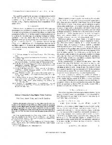
to the particular influence of interferences produced by cells using the same channel (co-channel interference): in a cell suffering only from co-channel interference, even though there is no traffic on it, the nodes may defer their transmissions if when sensing the medium, they detect other nodes using the channel from an interfering cell; these nodes are called exposed terminals The presence of adjacent channel interference reduces the effective SINR (Signal to Interference and Noise Ratio) and therefore, the number of errors in reception is increased. These effects used to be minimized with a good network design, prior to its deployment [2][3]: the best access point locations, transmitted powers and channel allocations are computed off-line in order to obtain the best performance at the same time that the sufficient capacity and a full coverage is guaranteed. IEEE 802.11 networks operate in the 5GHz (.11a) and 2.4GHz (.11b/g) unlicensed frequency bands. Communications in these bands need to implement spread spectrum techniques and limit their transmitted power in order to minimize the impact of interference with other devices. Once spread, the resulting signal occupies a bandwidth of about 20 MHz. In addition, the available channels are defined with 5MHz separation between consecutive carriers, bringing the need to use, at least, five channels of separation to guarantee that two simultaneous transmissions do not interfere with each other. Consequently, whereas there are up to 19 (12 in USA) non-overlapping channels in the 5GHz band, in the 2.4GHz band only three out of 13 (11 in USA) are nonoverlapping (traditionally, channels 1, 6 and 11) as shown in fig. 1. Bearing in mind the scenarios mentioned before, where the density of nodes can be very high, only three channels are not enough to guarantee an innocuous coexistence between different WLANs. Previous empirical studies stated that a separation of four channels can be used without reducing the performance [4], so the possibilities could be opened to channels 1, 5, 9 and 13 (where available). The idea of using all available channels appears in [5] for the first time. In this paper we present an analytical study on the effects of adjacent channel interference in IEEE 802.11abg WLANs which is supported by practical measurements and simulations. The

results provided are intended to assist different radio resource management mechanisms by providing hints on the use of partially overlapped channels, i.e. we can explain under what circumstances this practice is recommended. Similar studies focused on Direct Sequence Spread Spectrum have been previously published [6][7], but relayed on significant simplifications. The rest of the document is structured as follows: section II summarizes the operation of IEEE 802.11 MAC layer. In section III, the spectrum of IEEE 802.11 spread signals is analyzed. In section IV a model is presented that quantifies the amount of interference caused by partially overlapped channels. Section V quantifies the effect of interference on the network performance. In section VI some applicability statements are discussed, and finally, conclusions are given in VII. II.

IEEE 802.11 PROTOCOLS

The IEEE 802.11 MAC procedure [8] provides two operating modes: Distributed Coordination Function (DCF) and Point Coordination Function (PCF). The DCF uses the contention MAC algorithm CSMA/CA, whereas the PCF offers contention free access. The two modes can be used alternately in time. The DCF works as follows. Before initiating a transmission, a station senses the channel to determine whether it is idle or busy. If the medium is sensed idle during a period of time called Distributed Interframe Space (DIFS), the station is allowed to transmit. If the medium is sensed busy, the transmission is delayed until the channel is idle again. Physical and virtual carrier-sense functions are used to determine the state of the medium. Virtual carrier sense is referred to as the Network Allocation Vector (NAV). The NAV maintains a prediction of future traffic on the medium based on duration information that is announced in some frames. Basically, the physical layer provides a busy/idle medium recognition based on the detection of any energy above a given threshold Pth; physical layer can also report a busy medium upon detection of an 802.11 signal (above or below Pth). A slotted binary exponential backoff interval is uniformly chosen in [0, CW-1], where CW is the contention window. The backoff timer is decreased as long as the channel is sensed idle, stopped when a transmission is in progress, and reactivated when the channel is sensed idle again for more than DIFS. When the backoff timer expires, the station starts transmitting. After each data frame successfully received, the receiver transmits an acknowledgment frame (ACK) after a Short Interframe Space (SIFS) period. The value of CW is set

Figure 1: 2.4GHz ISM band

to its minimum value, CWmin, in the first transmission attempt, and ascends integer powers of two at each retransmission, up to a pre-determined value CWmax. The protocol described above is called basic or two-way handshaking mechanism. In addition, the specification also contains a four-way frame's exchange protocol called RTS/CTS mechanism: a station gains channel access through the contention process described previously, and sends a special frame called Request to Send (RTS), instead of the actual data frame. In response to that, the receiver sends a Clear to Send (CTS) frame after a SIFS interval. Subsequently, the requesting station is allowed to start the data frame's transmission after a SIFS period. The main objective of RTS/CTS handshake is the resolution of the hidden terminal problem. The mechanism is also employed to minimize the lost periods caused by collisions – the RTS frame is much shorter than data fames. Finally, the IEEE 802.11 DCF MAC protocol supports two kinds of Basic Service Set (BSS): the independent BSS, known as ad-hoc networks, which have no connection to wired networks, and the infrastructure BSS, which contains an AP connected to the wired network. The second kind of BSS assimilates to cellular networks with base stations. III. SPREAD SIGNALS The IEEE 802.11 defines different spreading techniques, but the devices that can be found today on the market are based on DSSS (Direct Sequence Spread Spectrum) and OFDM (Orthogonal Frequency Division Multiplexing). In DSSS, the data at the sending station is combined with a higher-rate bit sequence that spreads the user data in frequency by a factor equal to the spreading ratio. The IEEE 802.11 standards specify the use of Barker codes (1 and 2 Mbps) and the use of CCK (Complementary Code Keying in 5.5 and 11 Mbps) for the chip sequence in DSSS systems. The direct modulation effectively spreads the signal over a much wider bandwidth and its power spectrum can be described by the following equation:

 sin( 2π ·x )  2  PDSSS ( x ) =  2π ·x   1 

x≠0

(1)

x=0

where x is a function of the center frequency fc, and the bandwidth of the main lobe bm: x(fc,bm)=(f-fc)/bm. A general rule of thumb for DSSS systems is that the null to null bandwidth is 2x the chip rate. Since all DSSS modulations use a chip rate of 11 Mcps, the null to null bandwidth of the spread signal (bm) is 22MHz. In fig. 2, the spectrum defined by equation (1) is compared with Matlab simulations, consisting of a random symbol sequence that is created to represent the data to be transmitted; the data is then spread using the 11-bit Barker sequence and finally, a carrier wave is applied.

Consequently, a band-pass filter must be applied before transmitting to the medium. Moreover, a similar filter is applied in reception to isolate the desired signal from other sources. This way, the energy received from transmissions on adjacent channels is substantially reduced. In fig. 4, a Matlab simulation illustrates the effect of applying the spectrum mask by means of a 4th-order elliptic filter with 22MHz of bandwidth and a stop band 50dB down to a DSSS signal.

Figure 2: PSD of an unfiltered 802.11 DSSS signal

The IEEE 802.11a/g standards [9][10] specify an OFDM Physical Layer that splits an information signal across 52 separate sub-carriers. Four of the sub-carriers are pilot subcarriers that are used as a reference to disregard frequency or phase shifts. The remaining 48 sub-carriers provide separate wireless “pathways” for sending the information in a parallel fashion. The resulting sub-carrier frequency spacing is 0.3125 MHz (20MHz/64) and the total bandwidth is 20 MHz, but only 16.6MHz are actually occupied. According to the analysis in [11], the spectrum of the signal can be obtained summing the power spectra of all individual sub-carriers (Psk(f)). This power density is obtained directly from the Fourier transform of the time-window function defined by the standard:

W ( f ) = Ts

sin(πTs f ) cos(πTTR f ) − jπTs f · ·e πTs f 1 − 4TTR2 f 2

(2)

where Ts is the symbol duration (4μs), and TTR is the transition time, about 100 ns. The values for Ts and TTR are the same for all modulations. Then, for the kth sub-carrier Psk(f)=|W(f-0.3125k)|2/Ts; k= ±1; ±2;…; ±52/2. Note that the spectrum of any OFDM sub-carrier is only affected by the symbol shaping window and symbol rate. IV. MEASURING INTERFERENCE Logically, as the distance (in frequency) between two simultaneous transmissions increases, the effects of interference become less harmful. As explained above, in order to avoid interference, both transmissions should be separated by at least, five channels (> 22MHz). However, the IEEE 802.11 standard defines a transmit spectrum mask intended to limit the energy of the transmitted signal that invades adjacent channels: around fc, the signal is unmodified; at frequencies beyond fc±11MHz, the transmitted spectral products shall be less than –30 dBr, and 50 dBr for frequencies fc±22MHz. For OFDM, the transmitted spectrum shall have a 0 dBr bandwidth not exceeding 18 MHz, –20 dBr at 11 MHz frequency offset, –28 dBr at 20 MHz frequency offset and –40 dBr at 30 MHz frequency offset and above (see figures 3 and 4).

If we want to quantify the interference caused by transmissions in partially overlapped channels, we have to compute the PSD (Power Spectral Density) of the filtered signal. Assume a receiver tuned to fc, and a transmitter that is c channels apart. Also assume that the two devices use an identical filter for both transmission and reception; if the filter’s frequency response is represented by Ffc(f), where f is the frequency in MHz, the overlapping energy of the interfering signal is computed as: +∞

Pint = ∫ P( f )·Ffc ( f − 5c)·F fc ( f )df

(3)

−∞

P(f) = PDSSS(fc, 22) for DSSS and P(f) = ∑k Psk(f) for OFDM signals. Note that for our purposes, the integral can be done only in the region of interest, i.e. fc±22MHz. Thus, we quantify the interference caused by 802.11 transmissions, according to the attenuation of the filter for a specific channel, normalized by the amount of energy the receiver would get if tuned to that channel. In other words, if we call P0 the power that the receiver gets when both the receiver and the transmitter are on channel 1, and Pc is the new power obtained after moving the sender c channels away, the normalized loss factor is Pc / P0. In fig. 5 (and 6), Pc is the amount of energy received from channel 36 (3), and P0 the energy received from channel 34 (1). The following table contains the values in dB, obtained by means of Matlab simulations, and theoretically following equation (3) with perfect band-pass filters (bandwidth of 22MHz and a stop band 50dB down). Note that simulated values for OFDM attenuation are not included since the theoretical curves (2) were previously validated in [11]. TABLE I. ATTENUATION VALUES (IN DB) FOR ADJACENT CHANNELS c (ch. sep.) DSSS Th. DSSS Sim. OFDM Th.

0 0 0 0

1 0.28 0.37 0.55

2 2.19 1.79 2.46

3 8.24 8.03 6.60

4 25.50 23.47 34.97

5 49.87 53.21 51.87

For example, if a DSSS receiver is tuned to channel 1, it will receive all transmissions on channel 1 (c=0) without attenuation, but interfering transmissions produced in channel 4, are reduced by more than 8dB (c=3).

Figure 3: Spectral Density of 802.11 OFDM signal

Figure 5: OFDM Receiver tuned to ch. 34 filtering signals received in 34 and 36.

Figure 4: Spectral Density of 802.11 DSSS filtered signal

Figure 6: DSSS Receiver tuned to ch. 1 filtering signals received in 1 and 3.

A. Utilization The previous subsection showed how to evaluate the interference caused by transmissions in overlapping channels. Note that the spectrum densities studied correspond to activity periods, i.e. a snapshot taken when the transmitter is actually transmitting. It is therefore logical to draw the conclusion that a node that injects only a few frames per second is a source of interference that we can disregard in the presence of another node that is transmitting at the highest possible rate, even though the first station’s frames are received with much more energy than the latter’s. Therefore, the next step is to include the effect of utilization as a new parameter in order to consistently quantify interference from adjacent channels. Here, utilization is understood as the portion of time the node is actually transmitting into the air. To do so, the mean power received from a source in saturation state is taken as reference (considered utilization of 100%1). The measurement for every utilization degree is carried out with a spectrum analyzer, which covers 44MHz around the center frequency fc 10 times per second, taking samples every 100 kHz. The graph on fig. 7 shows the resulting average attenuation (normalized) equivalent to a given utilization degree. This equivalent attenuation is 1

Note that this utilization taken as reference does not actually correspond to a busy time of 100% due to backoff intervals and inter-frame spaces.

computed as the difference between the mean power received from a saturated station (no attenuation) and the mean power measured with lower utilizations. The values provided by the spectrum analyzer are directly proportional to the decay of the utilization. Thus, the attenuation in dB corresponds with the equation: 10·log10(u), where u represents the utilization (0 < u ≤ 1). That is to say, a utilization of 50% means that the source is transmitting half the time, and hence the averaged measured power is halved (i.e. the equivalent attenuation is 3 dB). We can now conclude our characterization of interference in partially overlapped channels with a complete example: if a receiver is tuned to channel 1, an interfering source continuously transmitting frames in channel 1 (c=0) will not be filtered. But if the transmitter moves to channel 4 (c=3) and reduces its utilization to 50%, we consider that the interference it produces is reduced on average by 8 (filter) + 3 (utilization) = 11 dB.

14

1,E+01

Measurements 1,E+00

10·log_10(u)

10

1,E-01

8 BER

Attennuation (dB)

12

6

1,E-02 1,E-03

4 2

1,E-04

0

1,E-05

m1

m2

m4

m5

m6

m7

m8

m3 0

20

40

60

80

100 1,E-06

Utilization (%)

0

Figure 7: Average attenuation equivalent to a given utilization obtained through experimental measurements

10

15

20

25

SINR (dB)

V. EFFECT OF NOISE AND INTERFERENCE ON PERFORMANCE

As mentioned before, a decrease in the SINR entails an increase of packet errors in reception. IEEE 802.11 standards define several sets of modulations and coding rates for the different physical layers. For example, IEEE 802.11b [12] specifies four modes: 11Mbps (8-bit CCK), 5.5Mbps (4-bit CCK), 2Mbps (DQPSK) and 1Mbps (DBPSK) to be used in the 2.4GHz frequency band. Each different scheme provides a different transmission rate, but the higher the chosen rate, the worse it performs in the presence of noise and interference; i.e. the harmful effects of interference are different for each different modulation and coding rate. The relationship SINR vs. BER (Bit Error Rate) can be derived either from empirical measurements (e.g. [13]) or using known formulas [14]. Figure 8 shows analytical curves with the bit error probability for all modulations in 802.11 OFDM under the assumption of binary convolutional coding and hard-decision Viterbi decoding with independent errors at the channel input (see details in [15]). An upper bound for the Packet Error Ratio (PER) was given in [16]:

PER = 1 − (1 − Pm ) 8l

5

(4)

where Pm is the error probability for data bits using the PHY mode m, and l is the frame length in Bytes. Once the PER is known, we can quantify the effect of interference on the saturation throughput as proposed in [17]: Chatzimisios et. al. introduced the PER into the well known Bianchi’s formulation [18]. In order to derive the effects of adjacent channel interference on the station’s performance, we can use the model described in IV with the exception of utilization. Even though the utilization model’s accuracy was validated with practical measurements with a spectrum analyzer, it is not applicable when the PER is computed from SINR values. The effects of utilization will depend not only on the activity/idle periods ratio, but also on the frame size distribution and the process describing inter-frame times in

Figure 8: Analytical BER vs. SINR curves of 802.11 OFDM transmissions in a Hard-decision Viterbi decoder for all 8 modes: 1 (6Mbps – BPSK), 2 (9Mbps BPSK), 3 (12Mbps QPSK), 4 (18Mbps QPSK), 5 (24Mbps 16-QAM), 6 (36Mbps 16-QAM), 7 (48Mbps 64-QAM) and 8 (54Mbps 64-QAM)

the interfering source. First of all, whenever the filtered signal is above Pth, the physical carrier sense mechanism will defer transmission for all interfering station’s frames, so in this case, the interference does not affect the PER and therefore there is no sense in applying the attenuation due to the utilization factor. Otherwise, the interference can be added to the SINR before deriving PER. Our estimation of PER is now: PERu = u·PER1; where PERu is the PER obtained with an adjacent interferer’s utilization of u and PER1, the PER when the interferer’s utilization is in saturation (u=1). This PER variation can be translated to an equivalent log10(1/u) increase in the SINR. These assumptions were verified by means of practical measurements and simulations. The simulated scenario consisted of two partially overlapping IEEE 802.11a cells with two stations each (tx and rx). Cell A’s rx receives 76dBm of unfiltered signal from cell B’s tx. The channel distance is 2 (ch. 34 and 36). B’s utilization is increased from 0 to 100% whereas A’s tx is always in saturation state. Simulations were made with two different modes (m=4 and m=8) in order to verify that our assumptions are independent of the modulation used. The details of the simulator’s PHY layer implementation can be found on [19]. The results are shown in fig. 9: dotted lines are obtained through analytical models with the saturation throughput computed using the formulas in [17] after deriving PER from u and SINR as explained before; solid lines are obtained from simulations. Practical measurements were made with a similar testbed but using DSSS devices with 1Mbps PHY (DBPSK); PER and SINR showed the same relationship.

35

18 Mbps Sim.

Sat. Throughput (Mbps)

30

18 Mbps Mod. 54 Mbps Sim.

25

54 Mbps Mod. 20

15

10

5

0 0

20

40

60

80

100

Utilization (%) in neighboring STA

Figure 9: Saturation throughput (Simulated vs. Analytical) in cell A when B’s transmitter changes its utilization in an adjacent channel (c=2).

To sum up, the computation of the interference used to obtain the PER differs from IV.A. In this case, recovering the complete example used to conclude section IV: if a receiver is tuned to channel 1, an interfering source continuously transmitting frames in channel 1 (c=0) will not be filtered. But if the transmitter moves to channel 4 (c=3) and reduces its utilization to 50%, we consider that the interference it produces, with regard to PER computation, is on average reduced 8 (filter) + 0.3 (utilization) = 8.3 dB. VI. APPLICABILITY Partially overlapped channels are a useful resort when the number of non-overlapping channels available is small. Thus, its applicability is mainly focused on the 2.4GHz band; recall that the number of non-overlapping channels is greater in the 5GHz band, and OFDM signals occupy a narrower effective bandwidth than DSSS. However, also note that not all the channels defined in the 5GHz band are non-overlapping.

A simple experiment can be carried out to illustrate why the use of partially overlapped channels could have a positive effect. The scenario consists of two totally overlapping WLAN cells, each composed of one 11b AP and one client station. Cell A reaches the saturation state (i.e. there is always a frame ready to be sent in the transmission buffer). Cell B’s offered throughput is increased from 0 to saturation. Figure 10 shows the carried throughput in A, measured at the application layer for different channel settings: while A remains in channel 1, B moves from 1 to 6. In figure 11, the same experiment is repeated after moving one of the cells 10m away to an adjacent room. It is clear that co-channel interference can be worse than adjacent-channel interference, depending on the cell utilization and the interfering signal level. For example, in the case that 4 or 5 channel separation is not possible due to a high density of WLANs, in the first scenario (figure 10), a network administrator would choose the same channel for both cells before setting partially overlapping channels. However, in the second scenario (figure 11) the received co-channel interference is still above Pth (-76 < Pth < -80 dBm) while a reduction of the interfering signal has led to an improved BER performance for adjacentchannel interference, to the point that a channel distance of 3 would be the best choice herein. For the same reason c=1 performs better than c=2 in the first scenario, but c=2 outperforms c=1 in the second. Thus, it is sometimes preferable to use partially overlapping channels. Knowing that the power of a signal that is received at a distance of d can be computed as Prx [dB] = G(c) + Ptx – k·10 log10(d) [20], where Ptx is the transmitted power, k a factor that depends on the environment (k=2 for open space), and G(c) a factor that captures the effect of different gain/loss elements (including tx/rx filters and antennas), isolating d:

d (c) = 10

(5)

7

A's carried throughput (Mbps)

7

A's carried throughput (Mbps)

G ( c ) + Ptx − Prx 10 k

6 5 4 3 2 1 0 0

1

2

3

4

5

6

6 5 4 3 2 1 0 0

Offered throughput in B (Mbps)

0

1

2

3

4

5

Offered throughput in B (Mbps)

1

Figure 10: Measured throughput in cell A with interference from different channels; both cells in the same room

Channel distance: 2 3

4

5

Figure 11: Measured throughput in cell A with interference from different channels; cells in adjacent rooms

6

we obtain dth when Prx=Pth, i.e. dth, which is also known as the carrier sense range, is the minimum distance between two nodes required to avoid the carrier sense mechanism to report a channel occupied when the other station is transmitting. Note that d(c) decreases with c, which means that the minimum distance required to avoid interference between two transmitters (due to CSMA/CA), is reduced by increasing the channel distance (dth(0) > dth(1) > … > dth(c)). Again we can say that it can be preferable to use partially overlapped channels before a channel that is already in use. Hence, the best channel assignment for an scenario like the one depicted in fig. 11 (with max(dxy) < dth(0)) will be that using channels 1, 5, 9 and 13. Observe that in this case, the use of partially overlapped channels avoids the exposed node problem [21].

RX2

d12 RX1

TX1

TX2

d24

d23

TX4

d14 RX4

d13 TX3

d34

RX3

Figure 12: Scenario with 4 .11b Tx/Rx pairs. All TXs are within carrier sense range of each other (dxy ) < dth(0)). RXs are only within range of their corresponding TX.

VII. CONCLUSIONS In this paper we have quantified the adjacent channel interference and its effect on the throughput performance in IEEE 802.11 WLANs using OFDM or DSSS. The methodology required to this quantification is as follows: the interfering signal is attenuated by tx/rx filters, depending on the channel distance according to Table I and this signal is further affected by 10·log10(u) dB depending on the interfering station’s utilization. On the other hand, one has to take into account that to quantify the effect on saturation throughput, the equivalent interfering filtered signal is affected by log10(u); this SINR is used to derive the PER, which in turn is used to obtain the saturation throughput. The results obtained from simulations, analytical models and practical measurements justify the use of partially overlapped channels instead of 3-coloring allocations traditionally applied to IEEE 802.11b networks. The proposed model can also be used in different radio resource management mechanisms, such as transmitted power assignments or rate adaptation strategies. ACKNOWLEDGMENT This work was supported in part by DURSI, the ERDF, the Spanish Government through project TEC2006-04504 and the i2CAT foundation. REFERENCES [1]

[2]

[3]

A. Akella, G. Judd, S. Seshan, and P. Steenkiste, “Selfmanagement in chaotic wireless deployments,” 11th international Conference on Mobile Computing and Networking, MobiCom '05, September 2005. A. Hills, “Large-Scale Wireless LAN Design,” IEEE Communications Magazine, vol. 39, num. 11, pp. 98107, November 2001. R.C. Rodrigues, G.R. Mateus, A.A.F Loureiro, “On the Design and Capacity Planning of a Wireless Local Area Network,” Network Operations and Management Symposium, NOMS, (IEEE/IFIP, ed.), pp. 335-348, April 2000.

[4]

D. Leskaroski, and W.B. Michael. Frequency Planning and Adjacent Channel Interference in a DSSS Wireless Local Area Network (WLAN). Wireless Personal Communications: Bluetooth Tutorial and Other Technologies. pp. 169-180. Kluwer Academic Publishers, 2001. [5] E. Garcia, R. Vidal and J. Paradells. New Algorithm for Distributed Frequency Assignments in IEEE 802.11 Wireless Networks. 11th European Wireless Conference, vol. 1, pp. 211-217, April 2005. [6] A. Mishra, V. Shrivastava, S. Banerjee and W. Arbaugh. Partially Overlapped Channels Not Considered Harmful. ACM SIGMETRICS Performance Evaluation Review, vol. 34, 1, pp. 63-74, June, 2006. [7] M. Burton. Channel Overlap Calculations for 802.11b Networks. White Paper, Cirond Technologies Inc, November 2002. [8] IEEE 802.11. Standard for Telecommunications and Information Exchange Between Systems—LAN/MAN Specific Requirements—Part 11: Wireless Medium Access Control (MAC) and Physical Layer (PHY) Specifications. New York: The IEEE, Inc., 1999. [9] IEEE 802.11. Supplement to Standard for Telecommunications and Information Exchange Between Systems—LAN/MAN Specific Requirements— Part 11: Wireless Medium Access Control (MAC) and Physical Layer (PHY) Specifications: High-speed Physical Layer in the 5 GHz Band, 802.11a. The IEEE, Inc., 2003. [10] IEEE 802.11. Standard for Telecommunications and Information Exchange Between Systems—LAN/MAN Specific Requirements—Part 11: Wireless Medium Access Control (MAC) and Physical Layer (PHY) Specifications: Amendment 4: Further Higher Data Rate Extension in the 2.4 GHz Band, 802.11g. The IEEE, Inc., 2003. [11] C. Liu, F. Lee, “Spectrum modelling of OFDM signals for WLAN,” Electronics Letters, vol. 40, pp. 14311432, October 2004. [12] IEEE 802.11. Supplement to Standard for Telecommunications and Information Exchange

[13]

[14] [15]

[16]

Between Systems—LAN/MAN Specific Requirements— Part 11: Wireless Medium Access Control (MAC) and Physical Layer (PHY) Specifications: Higher-Speed Physical Layer Extension in the 2.4 GHz Band, 802.11b. The IEEE, Inc., 2003. HFA3863: Direct Sequence Spread Spectrum Baseband Processor with Rake Receiver and Equalizer. Intersil Inc., December 2001. J.G. Proakis. Digital Communications. MCGraw-Hill, 4th ed. 2001. D. Qiao, S. Choi, K. G. Shin, “Goodput analysis and link adaptation for IEEE 802.11a wireless LANs”, IEEE Transactions on mobile computing, Vol.1, No. 4, pp. 278 – 292, December 2002. M. B. Pursley, D. J. Taipale, “Error probabilities for spread-spectrum packet radio with convolutional codes and Viterbi decoding”, IEEE Transactions on communications, Vol. COM-35, No. 1, pp. 1-12, January 1987.

[17] P. Chatzimisios, A. Boucouvalas and V. Vistas, “Infuence of channel BER on IEEE 802.11 DCF,” Electronics Letters, vol. 39, pp. 1687-1689, November 2003. [18] G. Bianchi, “Performance analysis of the IEEE 802.11 Distributed Coordination Function,” IEEE Journal on Selected Areas in Communications, vol. 18, pp. 535547, March 2000. [19] E. Lopez, J. Casademont, J. Cotrina, “Outdoor IEEE 802.11g Cellular Network performance”, in Proc. of IEEE Globecom04, November 2004. [20] T.S. Rappaport. Wireless Communications Principles and Practices. Prentice Hall PTR, 2nd ed., December 2001. [21] K. Heck. Wireless LAN performance in overlapping cells. IEEE 58th Vehicular Technology Conference, VTC'03-Fall, vol. 5, pp. 2895-2900, October 2003.