Applied Mathematics, 2011, 2, 271-282 doi:10.4236/am.2011.23032 Published Online March 2011 (http://www.SciRP.org/journal/am)
Effect of Point Source, Self-Reinforcement and Heterogeneity on the Propagation of Magnetoelastic Shear Wave Amares Chattopadhyay, Shishir Gupta, Abhishek K. Singh, Sanjeev A. Sahu Department of Applied Mathematics, Indian School of Mines, Dhanbad, India E-mail:
[email protected] Received October 1, 2010; revised November 1, 2010; accepted November 5, 2010
Abstract This paper investigates the propagation of horizontally polarised shear waves due to a point source in a magnetoelastic self-reinforced layer lying over a heterogeneous self-reinforced half-space. The heterogeneity is caused by consideration of quadratic variation in rigidity. The methodology employed combines an efficient derivation for Green’s functions based on algebraic transformations with the perturbation approach. Dispersion equation has been obtained in the closed form. The dispersion curves are compared for different values of magnetoelastic coupling parameters and inhomogeneity parameters. Also, the comparative study is being made through graphs to find the effect of reinforcement over the reinforced-free case on the phase velocity. It is observed that the dispersion equation is in assertion with the classical Love-type wave equation in the absence of reinforcement, magnetic field and heterogeneity. Moreover, some important peculiarities have been observed in graphs. Keywords: Shear Wave, Magnetoelastic, Self-reinforcement, Dispersion Equation, Seismic Wave
1. Introduction The study of mechanical behaviour of a self-reinforced material has great importance in Geomechanics. Many elastic fibre-reinforced composite materials are strongly anisotropic in behaviour. It is desirable to study the shear wave propagation in anisotropic media, as the propagation of elastic waves in anisotropic media is fundamentally different from their propagation in isotropic media. As the earth’s crust and mantle are not homogeneous, it is also interesting to know the propagation pattern of shear waves due to point source in heterogeneous medium. The characteristic property of a self-reinforced material is that its components act together as a single anisotropic unit as long as they remain in elastic condition (i.e. the two components are bound together so that there is no relative displacement between them). Selfreinforced materials are a family of composite materials, where the polymer fibres are reinforced by highly oriented polymer fibres, derived from the same fibre. Alumina or concrete is an example of self-reinforced material. Under certain temperature and pressure some fibre materials may also be modified to self-reinforced materials by Copyright © 2011 SciRes.
reinforcing a matrix material of the same fibre. In real life the fibres might be carbon, nylon, or conceivably metal whiskers. It has been observed that the propagation of elastic surface waves is affected by the elastic properties of the medium, through which they travel (Achenbach [1]). The Earth’s crust contains some hard and soft rocks or materials that may exhibit self-reinforcement property, and inhomogeneity is trivial characteristic of the Earth. These facts motivate us towards this study. The idea of introducing a continuous reinforcement at every point of an elastic solid was given by Belfield et al. [2]. Later Verma and Rana [3] applied this model to the rotation of tube, illustrating its utility in strengthening the lateral surface of the tube. Verma [4] also discussed the propagation of magnetoelastic shear waves in self-reinforced bodies. The problem of magnetoelastic transverse surface waves in self-reinforced elastic solids was studied by Verma et al. [5]. Chattopadhyay and Chaudhury [6] studied the propagation, reflection and transmission of magnetoelastic shear waves in a self-reinforced elastic medium. Chattopadhyay and Chaudhury [7] studied the propagation of magnetoelastic shear waves in an infinite self-reinforced plate. Chattopadhyay and Venkateswarlu AM
272
A. CHATTOPADHYAY
[8] investigated a two-dimensional problem of stress produced by a pulse of shearing force moving over the boundary of a fiber-reinforced medium. Choudhary et al. [9] studied transmission of shear waves through a selfreinforced layer between two inhomogeneous elastic half-spaces. Choudhary et al. [10] also discussed the plane SH wave response from elastic slab interposed between two different self-reinforced elastic solids. Recently, Chattopadhyay et al. [11] has shown that the propagation of Torsional waves in fibre-reinforced material is also possible. A class of interesting problem is concerned with an initially undisturbed body, which in its interior and at a specified time t = 0, is subjected to external disturbances. The external disturbances give rise to wave motions propagating away from the disturbed region. In seismology the problem of the source mechanism consists in relating observed seismic waves to the parameters that describes the source. In the Earth, neglecting the force of gravity, body forces in the equation of motion may be used to represent the processes that generate earthquakes. In general, these forces are functions of the spatial coordinates and time, may be different for each earthquake and are defined only inside a certain volume. The time dependence of these forces simplifies the solution of many problems in seismology. A type of body forces of great importance in the solution of many problems of elastodynamics is that formed by a unit impulsive force in space and time with an arbitrary direction; this point action or impulse is usually described by the Dirac delta function. Thus the solutions of equations of motion represent the elastic displacement due to a unit impulse force in space and time. For this reason, the Green’s function called the response of the medium to an impulsive excitation. The form of this function depends on the characteristics of the medium, its elastic coefficients, and its density. In a finite medium, it depends also on the shape of the volume and the boundary conditions on its surface. For each medium there is a different Green’s function that defines how this medium reacts mechanically to an impulsive excitation force and is, therefore, a proper characteristic of each medium. Green’s functions play an important role in the solution of numerous problems in the mechanics and physics of solids. Articles on application of Green’s function to seismological problems have been published in a wide range of journals attracting the attention of both researchers and practitioners with backgrounds in the mechanics of solids, applied physics, applied mathematics, mechanical engineering and material science. However, no extensive, detailed treatment of this subject has been available upto the present. The complete problem of Green’s function corresponds to an impulsive force in an arbitrary direction (Aki and Richards [12]). The propaga-
Copyright © 2011 SciRes.
ET
AL.
tion of Love type waves from a point source in either homogeneous or inhomogeneous elastic media has been considered by a number of authors. Notable are De Hoop [13], Brekhovskikh and Godin [14] Vrettos [15,16], Singh [17], Deresiewiez [18], Ewing et al. [19] etc. The propagation of Love waves due to point source in a homogeneous layer overlying a semi-homogeneous substratum has been discussed by Sezawa [20]. Sato [21] studied the propagation of SH waves in a double superficial layer over heterogeneous medium by taking variation in rigidity. Ghosh [22] studied the propagation of Love waves from the point source at the interface between an upper layer and a semi-infinite substratum; one medium is characterised by a slow linear variation in rigidity. Bhattacharya [23] described the possibility of the propagation of love type waves in an intermediate heterogeneous layer lying between two semi-infinite isotropic homogeneous elastic layers. Chattopadhyay and Kar [24] discussed the Love waves due to a point source in an isotropic elastic medium under initial stress. Covert [25] indicated a method for finding the Green’s function for composite bodies. Chattopadhyay et al. [26] studied the dispersion equation of Love waves in a porous layer. They used the Green’s function technique to obtain the dispersion equation. Watanabe and Payton [27] discussed the Green’s function for SH waves in a cylindrically monoclinic material. He derived the closed form expression for Green’s function for a few limited values of anisotropic parameters and shown the contours of the displacement amplitude for the time harmonic wave. Manolis and Bagtzoglou [28] described a numerical comparative study of wave propagation in inhomogeneous and random media. He employed the Green’s function approach for waves propagating from a point source, while techniques to account for the presence of boundaries are also discussed. Awojobi and Sobayo [29] discussed the ground vibrations due to seismic detonation of a buried source. Kausel and Park [30] used a sub-structuring technique to obtain the impulse response in the wave number-time domain for a layered half-space. Manolis and Shaw [31] developed the fundamental Green’s function for the case of scalar wave propagation in a stochastic heterogeneous medium. The present paper investigates the propagation of SH waves due to a point source in a magnetoelastic self-reinforced layer lying over a heterogeneous self-reinforced half-space. The heterogeneity is caused by consideration of quadratic variation in rigidity. The methodology employed combines an efficient derivation for Green’s functions based on algebraic transformations with the perturbation approach. Dispersion equation has been obtained in the closed form. The dispersion curves are compared for different values of magnetoelastic coupling parameters and inhomogeneity para-
AM
A. CHATTOPADHYAY
meters. Also, the comparative study is being made through graphs to find the effect of reinforcement over the reinforced-free case on the phase velocity. It is observed that the dispersion equation is in assertion with the classical Love-type wave equation in the absence of reinforcement, magnetic field and heterogeneity.
2. Formulation and Solution of the Problem We have considered a magnetoelastic self-reinforced layer of thickness H lying over a heterogeneous selfreinforced half-space. The x-axis has been taken along the propagation of waves and z-axis is positive vertically downwards as shown in Figure 1. The source of disturbance S is taken at the point of intersection of the interface of separation and z-axis. At first, we need to find the equation governing the propagation of SH wave in self reinforced magnetoelastic crustal layer. The constitutive equations used in a self-reinforced linearly elastic model are (Belfield et al. 1983)
ij ekk ij 2 T eij * ak am ekm ij ekk ai a j
2 L T ai ak ekj a j ak eki ak am ekm ai a j (1) *
i, j , k , m 1, 2,3
where ij are components of stress, eij components of infinitesimal strain, ij Kronecker delta, ai components of a , all referred to rectangular cartesian co-ordinates xi a a1 , a2 , a3 is the preferred directions of reinfor cement such that a12 a2 2 a32 1 . The vector a may be function of position. Indices take the values 1, 2, 3 and summation convention is employed. The coefficients , T , * , * and 2 L T are elastic constants with dimension of stress. T can be identified as the shear modulus in transverse shear across the preferred direction, and L as the shear modulus in longitudinal shear in the preferred direction. * and * are specific stress components to take into account different layers for concrete part of the composite material. The model considered here is of transversely isotropic material, also z=0
z=H
Figure 1. Geometry of the problem. Copyright © 2011 SciRes.
ET
AL.
273
known as materials of hexagonal symmetry. Equations governing the propagation of small elastic disturbances in a perfectly conducting self-reinforced elastic medium having electromagnetic force J B (the Lorentz force, J being the electric current density and B being the magnetic induction vector) as the only body force are 2u (2) ij , j J B 2i i t where J B is the xi -component of the force i J B and is the density of the layer. Here inte-
raction of mechanical and electromagnetic fields is considered. Let ui u1 , v1 , w1 and denoting x1 x, x2 y , x3 z then Equation (2) can be written as 11 12 13 2u J B 21 x x y z t 12 22 23 2 v J B 21 y x y z t 13 23 33 2 w J B 21 z x y z t
(3)
For SH wave propagating in the x-direction and causing displacement in the y-direction only, we shall assume that u1 w1 0, v1 v1 x, z , t and
0. y
Using Equation (4) in Equation (3), we have 12 23 2v J B 21 y x z t where
12 T
v1 v v L T a1 a1 1 a3 1 x z x
23 T
v1 v v L T a3 a1 1 a3 1 z z x
(4)
(5)
For stresses 12 and 23 , the first part indicate the shear stress due to elastic members (steel) and the second part indicates effect of comparatively non-elastic material of the composite section in the same direction. The first component would be having the term T , which can be termed as elastic coefficient and L T in the second term amounts for the effect comparatively non-elastic portion of the composite material. The well known Maxwell’s equations governing the electromagnetic field are AM
A. CHATTOPADHYAY
274
B B 0, E , H J , t (6) u i B e H and J E B . t where E is the induced electric field, J is the current density vector and magnetic field H includes both primary and induced magnetic fields. e and are the induced permeability and conduction coefficient respectively.
The linearized Maxwell’s stress tensor ij0
Mx
Let
x
y
i
z
j
j i
i
k k
and
H y t
1
2
3
i
is the
H x H z 0, t t
(13)
2 H J B e H H . 2
1
(14)
2 2 2 v1 2 v1 1 v1 1 v1 Q R , xz z 2 x 2 t 2
(15)
where
(9)
and v v Hx 1 Hz 1 t t . t x z
v1 v H 0 sin 1 . x z
H 2 Considering H H H . H and 2 the Equations (6), we get
P
(8) For perfectly conducting medium, (i.e. ), it can be seen that Equations (8) become
(10)
Assuming that primary magnetic field is uniform throughout the space. It is clear from Equation (10) that there is no perturbation in H x and H z , however from Equation (10) there may be perturbation in H y . Therefore, taking small perturbation, say b2 in H y , we have H x H 01 , H y H 02 b2 and H Z H 03 , where H , H , H are components of the initial magnetic 01 02 03 field H 0 . Copyright © 2011 SciRes.
(12)
Using the Equations (1) and (14), we obtain the equation of the motion for the magnetoelastic self-reinforced layer as
2 H x , 2 Hz , v v Hx 1 Hz 1 1 t t 2 H y . x z e
H y
v v H 0 cos 1 H 0 sin 1 b2 t t . t x z
b2 H 0 cos
In component form, Equation (7) can be written as
H z 1 t e
(11)
We shall consider initial value of b2 to be zero. Using Equation (11) in Equation (10), we get
ij
change in the magnetic field. In writing the above equations, we have neglected the displacement current. From Equation (6), we get H ui (7) 2 H e H . t t
H x 1 t e
crosses the magnetic field. Thus we have H H 0 cos , b2 , H 0 sin
Integrating with respect to t , we get
H b H b H b . H H , H , H and b b , b , b . b e
AL.
We can write H 0 H 0 cos , 0, H 0 sin , where H 0 H 0 and is the angle at which the wave
due to
the magnetic field is given by 0 Mx ij
ET
1 P T a32 L T e H 02 sin 2 , 1 Q T a12 L T e H 02 cos 2 and R 1 2a1a3 L T e H 02 sin 2 .
(16)
If 1 r , t be the force density distribution in the upper layer due to the point source, the equation of motion for SH wave propagation along x-axis becomes as 2 v1 Q 1 2 v1 R 1 2 v1 2 v1 4 1 r , t (17) 1 z 2 P 1 x 2 P 1 xz P 1 t 2 P
where r is the distance from the origin, where the force is applied to a point of coordinates and t is the time. Considering v1 x, z , t V1 x, z eit and 1 r , t 1 r eit in Equation (17), we obtain 4 1 r 2V1 Q 1 2V1 R 1 2V1 2 V1 1 z 2 P 1 x 2 P 1 xz P 1 P
(18)
where kc is the angular frequency, k the wave number and c is the phase velocity. Here the disturbances caused by the impulsive force 1 r may be represented in terms of Dirac-delta function at the source AM
A. CHATTOPADHYAY
point as 1 r x z H Therefore the equation of motion for the upper magnetoelastic self-reinforced layer with an impulsive point source is 4 x z H V1 Q V1 R V1 1 1 1 V1 2 2 1 z P x P xz P P (19) 1
2
1
2
2
ET
AL. 2
f 2 i
R0 P0
2
2
vr x, z e
P0
0
Vr , z e
i x
d
(21)
Now taking the Fourier transform of Equation (19), we obtain 2 z H d V1 dV f1 1 r12V1 4 1 z 2 1 dz dz P 2
(22)
R 1
P 1
, r12
2 P 1
2
L 2 L 0 z H 2
0
T T z H
P
and
P 1
(23)
2
where 0 is the density of the lower half-space,
(24)
, Q a and R 2a a .
P T a32 L T 2
2
2
T
2
2 1
2
1 3
2 L
2 L
2
2
T
2
T
In view of substitution v2 x, z , t V2 x, z eit and Equation (20), Equation (24) becomes 2
d V2 dV f 2 1 r22V2 4 2 z 2 dz dz
where Copyright © 2011 SciRes.
0 L
0 T
fr
z 2
in Equation (22) and
d 2V1 fz 2V1 4 1 z e 1 2 2 dz
(27)
d 2V2 f z 2V2 4 2 z e 2 2 dz 2
(28)
where
2
f12 f2 r12 , 2 2 r22 4 4
2
2 2 2 v2 v2 2 v2 2 v2 2 v2 Q R 2 z H 0 xz z z 2 x 2 t 2
2
0
T
Equation (25) for r 1, 2 respectively, we obtain
1
Now, the equation of motion for the lower heterogeneous self-reinforced elastic half-space is 2
1 3
Substituting Vr z Vr z e
Q
The heterogeneity of the lower inhomogeneous selfreinforced elastic half-space has been considered in the form
2
Now it is clear from Equation (25) that the displacement in the lower medium may be determined by assuming the lower medium to be homogeneous, isotropic having source density distribution 2 z .
where f1 i
0 L
2 1
2
Then the inverse transform can be given as
P0
Q a and R 2a a 0 T
0
1 vr x, z 2
2
P0 2 T 0 a32 L 0 T 0 ,
(20)
dx
P0
Q0
2
2 dV 2 d V2 2 2 z H 1 z H 2V2 z H 2 dz dz (26)
2
i x
2
0 2
Defining the Fourier transform Vr , z of vr x, z
, r2 2
4 2 z
2
as 1 Vr , z 2
275
(25)
The boundary conditions are f 1 dV P 1 1 V1 0, at z 0 2 dz V1 V2 , at z H
(29) (30)
f f 1 dV 2 dV P 1 1 V1 P 2 2 V2 , at z H (31) 2 2 dz dz
Thus Equations (27) and (28) together with prescribed boundary conditions (29) to (31) give the complete mathematical model for the problem. Now we apply Green’s function technique to solve it. If G1 z z0 is the Green’s function for the upper layer satisfying the condition dG1 0 at z 0 and at z H , then the equation sadz tisfied by G1 z z0 is d 2 G1 z z0 1 dz 2
2 G1 z z0 z z0
(32)
where z0 is a point in the upper medium and z is the field point. Multiplying the Equation (27) by G1 z z0 AM
A. CHATTOPADHYAY
276
and Equation (32) by V1 z , then subtracting and integrating with respect to z from z 0 to z H , we have f H dV 2 1 1 e 2 G1 H z0 V1 z0 (33) G1 H z0 1 dz z H P
Since
dG1 z z0 dz
0 at z 0 and z H . V1 z e
f 1 zH 2
dz
2
Replacing z0 by z and remembering that G1 H z G1 z H , the Equation (33) gives the value of V1 at any point z in the upper medium as V1 z
2 P
1
e
f1 H 2
dV G1 z H G1 z H 1 dz z H
2 dV1 z f1 V1 z 1 G1 z H G1 z H 2 dz z H P
2 G2 z z0 z z0
(35)
where z0 is the point in the lower medium, satisfying the condition
AL.
Therefore,
Now, let G2 z z0 be the Green’s function for the lower medium, as per previous discussion may be assumed to be homogeneous. We assume that G2 z z0 is the solution of the equation d 2 G2 z z0 1
ET
dG2 0 at z H and approaches to dz
(34)
zero as z . Multiplying Equation (28) by G2 z z0 and Equation (35) by V2 z , then subtracting and integrating with respect to z from z H to z , we have f2 z dV G2 H / z0 2 4 e 2 2 z G2 z z0 dz V2 z0 dz z H H
(36) Interchanging z by z0 in the Equation (36), the value of V2 z at any point z in the lower medium is
f 2 z0 dV V2 z G2 z H 2 4 e 2 2 z0 G2 z z0 dz0 dz z H H
Therefore, V2 z e
f z 2 2
f 2 z0 f2 H dV2 z f 2 V2 z 4 e 2 2 z0 G2 z z0 dz0 e 2 G2 z / H 2 H dz z H
(37)
With the help of boundary condition (30), we have 2 P 1
f H f 2 z0 2 dV z f1 dV z f 2 G1 H H G1 H H 1 V1 z G2 H H 2 V2 z 4 e 2 e 2 2 z0 G2 z / z0 dz 2 2 dz z H dz z H H
(38) Using boundary condition (31), Equation (38) can be written as f H f 2 z0 2 1 2 dV1 z f1 V1 z 1 G2 H H 4 e 2 e 2 2 z0 G2 H z0 dz0 2 H dz z H D1 P 0
where D1 is given in appendix I. dV z f1 Substituting the value of 1 V1 z from 2 dz z H V1 z e
f 1 zH 2
Equation (39) and 4 2 z0 from Equation (26) into Equation (34), we obtain
f H 2 2 2 G z H G H H e G1 z H 1 2 2 2 1 1 P0 G1 H H P G2 H H P0 G1 H H P G2 H H
2 dV 2 d V2 2 z0 H 2 z0 H 2 2 z0 H V2 z0 e 2 dz dz H 0 0
Copyright © 2011 SciRes.
(39)
f 2 z0 2
(40)
G2 H z0 dz0 AM
A. CHATTOPADHYAY
ET
AL.
277
In view of boundary condition (31), relation (37) gives V2 z e
f 2 zH 2
f z 2 2G1 H / H G2 z / H e 2 G2 z / H P 1 2 2 2 1 1 P0 G1 H / H P G2 H / H P0 P0 G1 H / H P G2 H / H
2 f22z0 dV2 2 d V2 2 2 2 z H z H V z G2 H / z0 dz0 z0 H 0 0 2 0 e 2 dz0 dz0 H
e
f z 2 2
2
P0
2 f22z0 dV2 2 d V2 2 2 z H 2 z H z H V z G2 z / z0 dz0 0 0 2 0 e 0 2 dz0 dz0 H
V2 z can be obtained from the relation (41) by the method of successive approximations. The value of V2 z obtained from Equation (41) when substituted in Equation (40) gives the value of V1 z . We are interested in the value of V1 z , which will give the displacement in the upper layer, and since the higher order of can be neglected; we take as the first order approximation
V1 z
(41)
2G1 z H G2 H H e 2
f 1 zH 2
1
P0 G1 H H P G2 H H
2 e
P
2
0
f 1 zH 2
V2 z
2G1 H H G2 z H e
f 2 zH 2
(42)
2
P0 G1 H H P 1 G2 H H
which gives the displacement at any point in the lower medium if it is taken as homogeneous. Putting this value of V2 z in Equation (40), we get G1 z H G1 H H
G1 H H P G2 H H 1
2
(43)
dG2 z0 H 2 2 d G2 z0 H 2 z0 H 2 z0 H 2 z0 H G2 z0 H G2 H z0 dz0 2 dz0 dz0 H
2
The solution of Equation (43) represents the elastic displacements due to a unit impulse force in space and time. Thus the Green’s function is the response of the medium to an impulsive excitation. If we know the values of G1 z H and G2 z H , then the value of V1 z can be determined from the Equation (43). We have assumed G1 z z0 as the solution of Equation (32). A solution of Equation (32) may also be obtained in the following manner. We have the equation d 2 (44) 2 0. dz 2 Two independent solutions of Equation (44), vanishing at z and z are 1 z e z and 2 z e z . Therefore the solution of the Equation (44) for an infinite medium is 1 z 2 z0 for z z ,
W
0
1 z 0 2 z W
for z z0 ,
where W 1 z 2 z 1 z 2 z 2 0.
So, the solution of Equation (32) is
e
z z0
.
2 Since G1 z z0 is to satisfy the condition dG1 0 at z 0 and z H dz
(45)
Therefore, we can assume that G1 z z0 C1e z C2 e z
e
z z0
2
.
where C1 and C2 are the arbitrary constants which can be evaluated using condition (45). We finally get
H z 0 H z H z H z z e z e 0 e 0 e 0 1 z z 0 e e G1 z z0 e 2 e H e H e H e H
.
(46)
Therefore, Copyright © 2011 SciRes.
AM
A. CHATTOPADHYAY
278
G1 z H
1 e z e z e H e H
,
ET
AL.
1 z z0 z z 2H e 0 , e 2
G2 z z0
(47)
and so
1 e H e H G1 H H H , e e H
G2 H z0
(48)
e
z0 H
(50)
G2 H H
Similarly, the value of G2 z / z0 can be written as
(49)
1
(51)
.
Substituting all these values in Equation (43), we get
V1 z
2e 2
H
P0 e
f 1 zH 2
e
H
z
e
e
z
P e 1
H
2 e H e H 1 2 1 2 H H P 1 e H e H 4 P0 e e
e H
(52)
Neglecting the higher powers of the Equation (52) may be approximated as 2e
V1 z 2
f 1 zH 2
P0 e H e H P e H e H 1
e
z
e z
2 H H e e 1 2 1 2 1 H H P e H e H 4 P0 e e
(53)
Taking the inverse Fourier transform of Equation (53), the displacement in the upper medium may be obtained as
e
V1 z 2
f 1 zH 2
2
H
P0 e
e
H
P e 1
H
e
H
e
z
e z ei x d
2 H H e e 1 2 1 2 1 H H P e H e H 4 P0 e e
(54)
The dispersion equation of SH waves will be obtained by equating to zero the denominator of the above integral, i.e.
2
P0 e H e H P e H e H 1
2 e H e H 1 2 1 2 H H P 1 e H e H 4 P0 e e
In view of the substitutions ik1 and k 2 the above Equation (55) gives the dispersion relation of
tan kH 1
P0 2 2
1
P 1
1 4k 1 2 P 2
1 1 2 2 Q0 R0 P0 2 2 P0 2
0.
(55)
shear waves in magnetoelastic self-reinforced layer lying over heterogeneous self-reinforced half-space 2
2
0 L 1 0 T
c 2 Q 2 R 2 1 a32 0 2 0 2 2P P0 0
. 2 2 2
(56)
where Copyright © 2011 SciRes.
AM
A. CHATTOPADHYAY
1 , 2 1 and 2 are given in the appendix I.
AL.
279
we take the following data 1) For Magnetoelastic Self-reinforced layer, [Markham [32]]
3. Particular Cases
L 5.66 109 N/m 2 , T 2.46 109 N/m 2 , 1 7,800 Kg/m3 .
3.1. Case I When 0 the dispersion relation (56) reduces to tan kH 1
P0 2
.
P 1 1
Moreover the following data are used (Hool and Kinne [33]; Maugin [34])
which is the dispersion equation of shear waves for the case of magnetoelastic self-reinforced layer lying over a homogeneous self-reinforced half-space due to a point source.
3.2. Case II When 0, L T 1 and L T 2 the dispersion relation (56) reduces to 0
0
1/ 2
c2 tan kH 2 1 2 3 1 H sin
1/ 2
c2 2 1 2 4
1/ 2
c2 1 1 H sin 2 1 2 3 1 H sin 2
2) For Heterogeneous Self-reinforced half space, [Chattopadhyay and Chaudhury [6]] L 0 7.07 109 N/m 2 , T 0 3.5 109 N/m 2 , 2 1, 600 Kg/m3 .
2
ET
where H , 3 and 4 are given in the appendix I. which is the dispersion equation of shear waves for the case of isotropic magnetoelastic layer lying over a homogeneous isotropic half-space due to a point source.
a1 0, 0.00316227, H 0.0, 0.05, 0.1,
The effect of reinforcement, magnetic field and heterogeneity on the propagation of plane SH waves in a magnetoelastic self-reinforced layer lying over an heterogeneous self-reinforced half spaces has been depicted by means of graphs. Figures 2 and 3 gives the variation of non-dimensional phase velocity c 1 with respect to non-dimensional wave number kH for different values of inhomogeneity and magnetoelastic coupling parameters H respectively. The small change in the non-dimensional wave number produces substantial change in non-dimensional phase velocity in both the cases. In each of these figures graphs are drawn for both in the presence and absence of reinforcement. In both the figures solid line curve 1, 2 & 3 refers to the case of reinforcement where as dotted line curves 4, 5 & 6 correspond to the reinforced free case. The comparative study of the graphs reveals that with the increase in heterogeneity and magnetoelastic coupling parameter, the phase velocity increases for both reinforced and reinforced free cases. It is important to add that the impact of reinforcement is dominant on the reinforced free case. 2.4
=0.00316227, =0.0 1:1:a1a= 1 0.00316227, = 0.0
3.3. Case III
2:2:a1a=1=0.00316227, 0.00316227, =0.25 = 0.25
2.2
When 0, H 0, L T 1 and L T 2 the dispersion relation (56) reduces to 0
=0.50 3:3:a1a=1=0.00316227, 0.00316227, = 0.50
0
4:4:a1a1==a a33=0.0, = 0.0,=0.0 = 0.0
2
a33=0.0, = 0.0,=0.25 = 0.25 5:5:a1a1==a
1
which is the classical Love wave equation.
c 1 c/ 1
1/ 2
2 c tan kH 2 1 3
1.6
For the case of a magnetoelastic self-reinforced layer lying over a non-homogeneous self-reinforced half space, Copyright © 2011 SciRes.
3
2 4 5
1.4
6
1.2
1
4. Numerical Examples
6:6:a1a1==a a33=0.0, = 0.0,=0.50 = 0.50
1.8
1/ 2
c2 2 1 2 4 1/ 2 c2 1 2 1 3
H2 0.0, 0.25, 0.5 T
0
0.5
1
1.5
2
2.5
3
kH kH
Figure 2. Dimensionless phase velocity against dimensionless wave number for ε H = 0.0 in presence and absence of reinforcement. AM
A. CHATTOPADHYAY
280 2.4
1:1:a1a= =0.00316227, 0.00316227, H ==0.0 0.0 1 H
2.4
0.00316227, HH==0.10 0.10 3:3:a1a=1=0.00316227,
2.2
2:2:a1a= =0.00316227, 0.00316227, H = 0.05 H=0.05 1
2.2
ET
4:4:a1a=1=a a33==0.0, 0.0, HH=0.0 = 0.0
2 1
=0.0, =0.0, =0.0 1: 1: a1 a=1a=a 3 = 3 0.0, = 0.0, HH = 0.0
=0.0, =0.0, =0.1 2:2: a1 a=1a=a 3 = 3 0.0, = 0.0, HH = 0.1 =a =0.0, =0.5, H=0.1= 0.1 3:3: a1 a== 1 a33 = 0.0, = 0.5, H
=0.00316227, =0.0, 4:4: a1 a=10.00316227, =0.0, HH==0.0 0.0
2
5:5:a1a=1=a a33==0.0, 0.0, HH=0.05 = 0.05
5:5: a1 a=10.00316227 , =0.0, HH==0.1 0.1 =0.00316227, =0.0,
4
a33==0.0, 0.0, HH=0.10 = 0.10 6:6:a1a=1=a
6:6: a1 a= 0.00316227 , =0.5, HH==0.1 0.1 =0.00316227, =0.5, 1
1.8
c/ 1
1.8
AL.
c 1
c/ 1
c 1
1.6
1.6 1
4 1.4 6
1
0
0.5
1
2
2
1.5
5
3 1.2
2
2.5
3
kH kH
Figure 3. Dimensionless phase velocity against dimensionless wave number for ε = 0.0 in presence and absence of reinforcement.
In Figure 4 curve 1 stands for the isotropic homogeneous layer lying over isotropic homogeneous half space, curve 2 stands for the isotropic magnetoelastic homogeneous layer lying over isotropic homogeneous half space, curve 3 stands for isotropic magnetoelastic homogeneous layer lying over isotropic heterogeneous half space, curve 4 stands for the self-reinforced homogeneous layer lying over a homogeneous self-reinforced half space, curve 5 stands for the magnetoelatic self-reinforced homogeneous layer lying over a homogeneous self-reinforced half space and curve 6 stands for the magnetoelatic self-reinforced homogeneous layer lying over a heterogeneous self-reinforced half space. The comparative study shows that as anisotropy prevails through self-reinforcement, magnetoelasticity prevails through magnetoelastic coupling parameter and heterogeneity prevails through inhomogeneity parameter in the medium, the phase velocity of the SH waves due to a point source gets supported more and more. It is also evident that the coupling parameters H and the heterogeneity both support the phase velocity but the effect of heterogeneity is prominent.
5. Conclusions Massive earth crust with built up RCC and Masonry infrastructures considerably influence the seismic waves propagation mainly due to elastic properties of the media. The present study has established that the phase velocity dispersion curve is affected by its magnetoelastic reinforced parameters and irregular boundaries. Ground shaking and earthquake loads can be visualized through this study. It is the fact that the earth crust and built up RCC and masonry structures over it will be proportionately afCopyright © 2011 SciRes.
6
1.4
5
1.2
3
1
0
0.5
1
1.5
2
2.5
3
kH kH
Figure 4. Dimensionless phase velocity against dimensionless wave number for different cases.
fected by the response of the ground motion for these wave propagation. RCC and masonry structures have dynamic properties like mass, stiffness and strength responsible for vibration parameters due to ground motion. Seismic forces are proportional to the mass of the structures and the acceleration caused by the ground movement. Frequency is the measure of how often ground motion changes direction. Amplitude is a measure of the magnitude of this motion. These parameters will be of great help for foundation design capable of translation. A well-designed and well-built RCC structure has a reliable load path that transfers these disturbing forces through the structures to the foundation where the soil can resist them. Besides earthquake, the ground motion may be due to heavy plant operation, blasting, rolling or falling of heavy masses. All these may cause harmonically forced vibration or transient vibration with impulse and arbitrary excitation to the reinforced media. For these conditions, there are well established methods to calculate principal modes of vibration and associated parameters. Wave propagation phenomenon in reinforced media is one of the most important information for the design and development of heavy civil construction projects. If the nature and sources of ground movement are predictable, then the design of RCC, masonry and steel structures for the construction of buildings, towers and bridges will be more accurate, scientific and safe. The present study has established that increase in heterogeneity and magnetoelastic coupling parameter increases the phase velocity for both reinforced and reinforced free cases. It is important to add that the impact of reinforcement is dominant on the reinforced free case. Hence the study of magnetoelastic shear wave propagation due to a point source in magnetoelastic self-reinforced layer over a heterogeneous self-reinforced half-space AM
A. CHATTOPADHYAY
provides valuable information for selection of proper structural materials for present day construction work.
6. Acknowledgements The authors convey their sincere thanks to Indian School of Mines, Dhanbad for providing JRF to Mr. Abhishek Kumar Singh and also facilitating us with its best facility. Acknowledgement is also due to DST, New Delhi for the providing financial support through Project No. SR/S4/ MS: 436/07, Project title: “Wave propagation in anisotropic media”.
ET
AL.
281
tween Two Different Self Reinforced Elastic Solids,” International Journal of Applied Mechanics and Engineering, Vol. 11, No. 4, 2006, pp. 787-801. [11] A. Chattopadhyay, S. Gupta, S. K. Samal and V. K. Sharma, “Torsional Wave in Self-Reinforced Medium,” International Journal of Geomechanics, Vol. 9, No. 1, 2009, pp. 9-13. doi:10.1061/(ASCE)1532-3641(2009)9:1(9) [12] K. Aki and P. G. Richards, “Quantitative Seismology: Theory and Methods,” W. H. Freeman & Co., New York, 1980.
7. References
[13] A. T. De Hoop, “Handbook of Radiation and Scattering of Waves: Acoustic Waves in Fluids, Elastic Waves in Solids, Electromagnetic Waves,” Academic Press, London, 1995.
[1]
J. D. Achenbach, “Wave Propagation in Elastic Solids,” North Holland Publication Company, New York, 1975.
[14] L. M. Brekhovskikh and O. A. Godin, “Acoustics of Layered Media,” Springer-Verlag, Berlin, 1992.
[2]
A. J. Belfield, T. G. Rogers and A. J. M. Spencer, “Stress in Elastic Plates Reinforced by Fibers Lying in Concentric Circles,” Journal of the Mechanics and Physics of Solids, Vol. 31, No. 1, 1983, pp. 25-54. doi:10.1016/0022-5096(83)90018-2
[3]
P. D. S. Verma and O. H. Rana, “Rotation of a Circular Cylindrical Tube Reinforced by Fibres Lying along Helices,” Mechanics of Materials, Vol. 2, No. 4, 1983, pp. 353-359. doi:10.1016/0167-6636(83)90026-1
[4]
P. D. S. Verma, “Magnetoelastic Shear Waves in SelfReinforced Bodies,” International Journal of Engineering Science, Vol. 24, No. 7, 1986, pp. 1067-1073. doi:10.1016/0020-7225(86)90002-9
[5]
P. D. S. Verma, O. H. Rana and M. Verma, “Magnetoelastic Transverse Surface Waves in Self-Reinforced Elastic Bodies,” Indian Journal of Pure and Applied Mathematics, Vol. 19, No. 7, 1988, pp. 713-716.
[6]
[7]
[8]
A. Chattopadhyay and S. Chaudhury, “Propagation, Reflection and Transmission of Magnetoelastic Shear Waves in a Self Reinforced Medium,” International Journal of Engineering Science, Vol. 28, No. 6, 1990, pp. 485-495. doi:10.1016/0020-7225(90)90051-J A. Chattopadhyay and S. Chaudhury, “Magnetoelastic Shear Waves in an Infinite Self-Reinforced Plate,” International Journal of Numerical and Analytical Methods in Geomechanics, Vol. 19, No. 4, 1995, pp. 289-304. doi:10.1002/nag.1610190405 A. Chattopadhyay and R. L. K. Venkateswarlu, “Stresses Produced in a Fibre-Reinforced Half Space Due to Moving Load,” Bulletin of Calcutta Mathematical Society, Vol. 90, 1998, pp. 337-342.
[9] S. Chaudhary, V. P. Kaushik and S. K. Tomar, “Transmission of Shear Waves through a Self-Reinforced Layer Sandwiched between Two Inhomogeneous Viscoelastic Half-Spaces,” International Journal of Mechanical Sciences, Vol. 47, No. 9, 2005, pp. 1455-1472. doi:10.1016/j.ijmecsci.2005.04.011 [10] S. Chaudhary, V. P. Kaushik and S. K. Tomar, “Plane SH-Wave Response from Elastic Slab Interposed be-
Copyright © 2011 SciRes.
[15] C. Vrettos, “Forced Anti-Plane Vibrations at the Surface of an Inhomogeneous Half-Space,” Soil Dynamics and Earthquake Engineering, Vol. 10, No. 5, 1991, pp. 230235. doi:10.1016/0267-7261(91)90016-S [16] C. Vrettos, “The Boussinesq Problem for Soil with Bound Nonhomogeneity,” International Journal of Numerical and Analytical Methods in Geomechanics, Vol. 22, No. 8, 1998, pp. 655-669. doi:10.1002/(SICI)1096-9853(199808)22:83.0.CO;2-R [17] K. Singh, “Love Waves Due to a Point Source in an Axially Symmetric Heterogeneous Layer between Two Homogeneous Half Spaces,” Pure and Applied Geophysics, Vol. 72, No. 1, 1969, pp. 35-44. doi:10.1007/BF00875690 [18] H. Deresiewich, “A Note on Love Waves in Homogeneous Crust Overlying an Inhomogeneous Substratum,” Bulletin of Seismological Society of America, Vol. 52, 1962, pp. 639-645. [19] M. Ewing, W. S. Jardetzky and F. Press, “Elastic Waves in Layered Media,” McGraw-Hill, New York, 1957. [20] K. Sezawa, “Love Waves Generated from a Source of a Certain Depth,” Bulletin of the Eathquake Research Institute, University of Tokyo, Vol. 13, 1935, pp. 1-17. [21] Y. Sato, “Love Waves Propagated upon Heterogeneous Medium,” Bulletin of the Eathquake Research Institute, University of Tokyo, Vol. 30, 1952, pp. 1-12. [22] M. L. Ghosh, “Love Wave Due to a Point Source in an Inhomogeneous Medium,” Gerlands Beitrage Zur Geophysik, Vol. 70, 1970, pp. 319-342. [23] J. Bhattacharya, “The Possibility of the Propagation of Love Type Waves in an Intermediate Heterogeneous Layer Lying between Two Semi-Infinite Isotropic Homogeneous Elastic Layers,” Pure and Applied Geophysics, Vol. 72, No. 1, 1969, pp. 61-71. doi:10.1007/BF00875693 [24] A. Chattopadhyay and B. K. Kar, “Love Wave Due to a Point Source in an Isotropic Elastic Medium under Initial Stress,” International Journal of Non-Linear Mechanics, Vo. 16, No. 3-4, 1981, pp. 247-258. AM
A. CHATTOPADHYAY
282 doi:10.1016/0020-7462(81)90038-X
ET
AL.
2, 2006, pp. 131-143. doi:10.1002/eqe.4290050203
[25] E. D. Covert, “Approximate Calculation of Green’s Function for Built-Up Bodies,” Journal of Mathematical Physics, Vol. 37, No. 1, 1958, pp. 58-65.
[30] E. Kausel and J. Park, “Impulse Response of Elastic Half-Space in the Wave Number-Time Domain,” Journal of Engineering Mechanics ASCE, Vol. 130, No. 10, 2004, pp. 1211-1222. doi:10.1061/(ASCE)0733-9399(2004)130:10(1211)
[26] A. Chattopadhyay, M. Chakraborty and V. Kaushwaha, “On the Dispersion Equation of Love Waves in a Porous Layer,” Acta Mechanica, Vol. 58, No. 3-4, 1986, pp. 125136. doi:10.1007/BF01176595
[31] G. D. Manolis and R. P. Shaw, “Wave Motions in Stochastic Heterogenous Media,” Engineering Analysis with Boundary Element, Vol. 15, No. 3, 1995, pp. 225-234. doi:10.1016/0955-7997(95)00026-K
[27] K. Watanabe and R. G. Payton, “Green’s Function for SH-Wave in Cylindrically Monoclinic Material,” Journal of Mechanics and Physics, Vol. 50, No. 11, 2002, pp. 2425-2439. doi:10.1016/S0022-5096(02)00026-1
[32] M. F. Markham, “Measurements of Elastic Constants of Fibre Composite by Ultrasonics,” Composites, Vol. 1, 1970, pp. 145-149. doi:10.1016/0010-4361(70)90477-5
[28] G. D. Manolis and A. C. Bagtzoglou, “A Numerical Comparative Study of Wave Propagation in Inhomogeneous and Random Media,” Computational Mechanics, Vol. 10, No. 6, 1992, pp. 397-413. doi:10.1007/BF00363995
[33] G. A. Hool and W. S. Kinne, “Reinforced Concrete and Masonry Structure,” McGraw-Hill, New York, 1924. [34] G. A. Maugin, “Review Article: Wave Motion in Magnetizable Deformable Solids,” International Journal of Engineering Science, Vol. 19, No. 3, 1981, pp. 321-388. doi:10.1016/0020-7225(81)90059-8
[29] A. O. Awojobi and O. A. Sobayo, “Ground Vibration Due to Seismic Detonation of a Buried Source,” Earthquake Engineering and Structural Dynamics, Vol. 5, No.
Appendix I P 1 D1 G1 H H 2 P R 1 1 1 2 P
G2 H H zH 1/ 2
2 c 2 Q 1 1 1 P P
2 2 c2 R Q , 2 0 2 20 0 2 2P P0 P0 0
2
1/ 2
T 0 H2 T 1 2 , 2 , 3 , 4 and H e 0 1 0 0 1
Copyright © 2011 SciRes.
AM