International Journal of Computer Applications (0975 â 8887). Volume 69â No.20, ... backpropagation (trainrp) is best in terms of speed and mean square error ...
International Journal of Computer Applications (0975 – 8887) Volume 69– No.20, May 2013
Effect of Training Algorithms on the Performance of ANN for Pattern Recognition of Bivariate Process Olatunde A. Adeoti
Peter A. Osanaiye
Department of Mathematics and Statistics Bowen University, Iwo Osun state, Nigeria
Department of Statistics University of Ilorin, Ilorin Kwara state, Nigeria
ABSTRACT Artificial Neural Network (ANN) which is designed to mimic the human brain have been used in the literature for identifying variable(s) that is(are) responsible for out-ofcontrol signal and the training algorithms have played a significant role in the identification of the aberrant variable(s). In this paper the effect of three algorithms in the training of ANN for pattern recognition of bivariate process is studied. Situations in which the algorithms performed satisfactorily with respect to recognition accuracy (in percentages), epochs and MSE were identified. The result of study shows that the Levenberg-Marquardt (trainlm) is the best algorithm for pattern recognition of bivariate manufacturing process in terms of recognition accuracy and the resilient backpropagation (trainrp) is best in terms of speed and mean square error performance.
Key words: Artificial neural network; training algorithms; feedforward multilayer perceptron; recognition accuracy
1. INTRODUCTION Many of the activities associated with the manufacturing process possess more than one quality variables which are usually correlated. Monitoring and controlling these quality characteristics using the traditional Shewhart univariate control charts would be ineffective for controlling the process as it ignores the correlation between the variables. To help overcome the problem, [14] first developed the multivariate control chart based on the T2 statistics for the monitoring of process with more than one quality characteristics. The Multivariate control chart developed capitalizes on the relationship that typically exists between variables which are usually correlated. Later, some other control charts to handle multivariate processes were proposed which include Hotelling’s T2 control chart [14]; MEWMA chart [16], [22] and MCUSUM charts [7], [13] and [24]. The problem with the multivariate control charts is that they always have difficulties in determining which variable or set of variables is responsible for the signal when the process is out of control. As a result different methods for the detection of the out-ofcontrol variables was developed to help identify aberrant variables; unfortunately, some of these methods still have some disadvantages in certain situations as discussed by [2], [4], [17] –[19] . Artificial Neural Network(ANN), one of the Artificial Intelligence (AI) tools in pattern recognition designed to mimic the human brain have proven to be an efficient alternative to the traditional methods of identifying aberrant variable in a multivariate process environment [6], [10], [20]. ANN consists of a set of computational units called neurons or nodes and a set of weighted, directed connections between these nodes. These variable weights connect nodes both in parallel and in sequence. The weights of the connections
determine the strength of the influence that one node has on the other nodes. The Artificial Neural Network is built with a systematic stepby-step procedure to optimize a performance criterion or to follow some implicit internal constraint, which is commonly referred to as the learning rule or process. The learning process involves updating network architecture and connection weights so that a network can efficiently perform a specific recognition task. In artificial neural networks, the designer chooses the network topology, the performance function, the learning rule and the training algorithms, and the criterion to stop the training phase, but the system automatically adjusts the parameters. Studies have shown that the most commonly used family of ANN for pattern recognition is the Feedforward Multilayer Perceptron (FFMLP) network [3], [20]. The FFMLP is an artificial neural network that performs nonlinear task and has three layers: input layer, one or more hidden layers and one output layer. The input layer nodes are unique in that their sole purpose is to distribute the input information to the next processing layer. The hidden layer nodes process all incoming signals by applying factors to them (termed weights) and the task of the output layer is to determine the patterns. Connections exist between the nodes of adjacent layers to relay the output signals from one layer to the next. Fully connected networks occur when all nodes in each layer receive connections from all nodes in each preceding layer. Information enters a network through the nodes of the input layer. Each layer also has an additional element called a bias node. Bias nodes simply output a bias signal to the nodes of the current layer All inputs to a node are weighted, combined and then processed through a transfer function that controls the strength of the signal relayed through the node’s output connections. These transfer functions set the output signal strength between -1 and +1 and also between 0 and 1 depending on the particular transfer function. The commonly used transfer functions are the hyperbolic tangent function and the sigmoid function. The functions are selectable on a layer- by-layer basis and networks can be created that incorporate multiple types. In this paper the effect of three training algorithms namely Levenberg-Marquardt, Resilient back-propagation and QuasiNewton algorithms on the performance of ANN models for pattern recognition of bivariate process is investigated and situations in which the algorithms performed satisfactorily with respect to recognition accuracy, epochs and MSE for varying number of nodes in the hidden layer chosen empirically between 10 and 20 were identified.
8
International Journal of Computer Applications (0975 – 8887) Volume 69– No.20, May 2013
2. NEURAL NETWORK TRAINING ALGORITHMS Three ANN training algorithms namely resilient backpropagation (trainrp), Quasi-Newton (trainbfg) and Levenberg-Marquardt (trainlm) are used and the output of the network is compared with a pre-specified target output in an attempt to minimize the differences between the network actual output and target output by adjusting the weights and biases. This is with a view of obtaining the best algorithm that produces ANN with high recognition accuracy, least global error, E and faster training for the pattern recognition of bivariate manufacturing process. The global error E is defined as
where
is the target output and
is the actual output
2.1 Resilient backpropagation Riedmiller [23] proposed the resilient backpropagation (trainrp) training algorithm to eliminate the effects of the magnitudes of the partial derivatives. In the trainrp, only the sign of the derivative is used to determine the direction of the weight update; the magnitude of the derivative has no effect on the weight update. The size of the weight change is determined by a separate update value. The performances however degrades as the error goal is reduced.
neural networks particularly its exact value. Therefore, the Quasi-Newton (trainbfg) which doesn’t require calculation of the Hessian matrix of second derivatives of the Newton method but consider at each iteration an approximation of the Hessian matrix specified by gradient evaluations that is suitably updated at each iteration of the algorithm was proposed by [9]. The update is computed as a function of the gradient.
2.3 Levenberg-Marquardt Algorithm The Levenberg–Marquardt (trainlm) algorithm [12] provides a numerical solution to the problem of minimizing a function (generally nonlinear) over a space of parameters of the function. It is fast and has stable convergence. The Levenberg-Marquardt algorithm blends the steepest descent method and the Gauss-Newton algorithm as it inherits the speed of the Gauss-Newton and stability of the steepest descent method. It was designed to approach second-order training speed without having to compute the Hessian matrix. [11]. When the performance function has the form of a sum of squares, the Hessian matrix, H, can be approximated as with the introduction of the Jacobian matrix and the gradient can be computed as where J is the Jacobian matrix that contains first derivatives of the network errors with respect to the weights and biases and e is a vector of network errors. When training with the LevenbergMarquardt algorithm, it uses the approximation to the Hessian matrix in the following Newton-like update:
2.2 Quasi- Newton Algorithm Dennis and Schnabel[9] proposed the Quasi-Newton (trainbfg) as improvement to the Newton’s algorithm for fast optimization as it often converges faster than conjugate gradient algorithm. The basic step function of the Newton algorithm was given as
where
is the weight update at time k+1
is the weight at current time k
is the Hessian matrix defined as
3. MATERIALS AND METHODS A. Generation of Input Dataset To perform a thorough pattern recognition study through training, validation and testing of the ANN model using the training algorithms required large multivariate correlated samples which ideally ought to be collected from real-world manufacturing process environment. Only when the ANN model is trained through suitable and appropriate dataset and algorithm can it acquire the ability to recognize the patterns of process mean vector. However, since they are not economically available simulation is an effective and useful alternative for generating dataset to identify normal/abnormal patterns in a manufacturing process environment. [1] investigated the use of different percentages of dataset allocation into training, validation and testing on the performance of ANN in pattern recognition of bivariate process and simulates the dataset from bivariate normal distribution when the variables are correlated. This approach is used in this paper. Let with mean
is gradient component defined as the first-order derivative of total error function given as
Unfortunately, it is complex and expensive to compute the Hessian matrix of the Newton’s method for feedforward
denote the bivariate normal distribution and variance-covariance matrix
where =1, for all i and = for all where is the correlation value between the two variables in each pattern. The in-control mean is assumed to be a zero vector. The variance-covariance matrix is assumed to be scaled so as to have unit variance for all components and we restrict our work to the shift in mean vector only. A small shift size is assigned to the shift magnitude. The data matrix for two process variables based on samples of 450 observations is generated for shift in the mean vector.
9
International Journal of Computer Applications (0975 – 8887) Volume 69– No.20, May 2013
B. Design of Artificial Neural Network Model The feedforward multilayer perceptron neural network (FFMLP) model which consists of one input layer, one hidden layer and one output layer was chosen as the model of interest. Figure 1 shows a FFMLP neural network model. Before this model can be put into application, it needs to be trained and tested. Supervised training approach was adopted for training the neural network. The raw data generated for each of the patterns were allocated into 80% (training), 10% (validation) and 10% (testing) and presented to the FFMLP network. The number of nodes in the input layer is the number of variables in the multivariate process i.e. p=2. Three output nodes are used in the output layer which is the number of classes. Also, the number of nodes in the hidden layer were selected empirically by varying the number of nodes between 10 and 20 for each of the training algorithm after trying various network structures since there is no reliable method for systematically determining them ([3], [5], [8]. All the network models for training have the same architecture and same dataset allocation.
4. RESULTS AND DISCUSSION After the network have been trained using the training set and appropriate weights for the difference between the target and actual output of the network model was obtained and saved. The trained neural network was used to test the performance of the network on test dataset of 45 patterns. The testing results of the networks in which the recognition accuracy, mean square error and number of iterations (epoch) for the effect of training algorithms on the performance of the ANN model are given in Tables 1, 2 and 3. The overall recognition accuracy for the three algorithms is shown in Table 4. Similarly, the number of nodes in the hidden layer that gave the lowest mean square error was determined for each network Table 1. Performance of Resilient backpropagation (Trainrp) algorithm on ANN model
NN configuration 2-10-3
Mean Square Error
Epoch
Recognition accuracy
2.28717E-8
10
80.7
2.20034E-8
18
80.4
2-12-3
1.87227E-8
14
81.3
2-13-3
1.60717E-8
9
81.3
2-14-3
8.26104E-9
14
72.2
2-15-3
1.90931E-10
9
76.7
2-16-3
4.30479E-11
19
81.6
2-17-3
8.76111E-9
13
75.8
Figure 1 A Feedforward Multilayer Perceptron (FFMLP) neural network model
2-18-3
2.95118E-7
5000
80.7
2-19-3
4.51216E-8
31
80.0
C. Neural Network Training
2-20-3
2.01198E-8
8
80.2
A set of 450 sample patterns are generated from the bivariate normal distribution and allocated into training, validation and testing dataset. The dataset are then randomized to avoid bias in the order of presentation to the ANN. During learning, a training data set (360 patterns) was used for weight updating, (45 patterns) for validating the network to avoid overfitting and (45 patterns) as test set for evaluating the generalization performance of the trained network to new data not seen before. The training of the network continues until one of the stopping criteria was satisfied: The performance error goal was achieved, that is, the mean square error gets sufficiently close to zero and/or the maximum allowable number of epochs was met.
When the resilient backpropagation was used in the training of the network, the entire model except ANN model 2-18-3 met the error goal criterion. Also, the best node in the hidden layer was found to be 16. The number of epochs when compared to other algorithms is consistently low for nodes less than 17 in the hidden layer and the speed is found to be generally the fastest.
2-11-3 Input layer ....... Hidden layer
Output layer
MATLAB M-files programming codes were written using the MATLAB Neural network toolbox software for the three selected training algorithms. The transfer functions used are the hyperbolic tangent function for the hidden nodes which transforms the layer inputs to output range from -1 to +1 and the sigmoid function for the output nodes that transforms the layer inputs to output range from 0 to 1 [8]. The maximum allowable number of epoch was 5000 and the performance error goal was set at while other parameters were kept constant when training for varying number of hidden nodes for the dataset of individual network.
Table 2. Performance of Levenberg-Marquardt (Trainlm) algorithm on ANN model
NN configuration
Mean Square Error
Epoch
Recognition accuracy
2-10-3
1.52738E-9
13
82.2
2-11-3
6.73207E-9
10
83.8
2-12-3
2.09837E-9
21
84.2
2-13-3
2.47557E-9
12
85.6
2-14-3
1.47433E-9
13
86.0
2-15-3
2.02957E-9
13
85.3
2-16-3
2.02842E-9
30
90.7
2-17-3
1.41797E-9
10
93.6
10
International Journal of Computer Applications (0975 – 8887) Volume 69– No.20, May 2013
2-18-3
1.53983E-9
15
91.8
2-19-3
1.47102E-9
16
92.2
2-20-3
3.41316E-9
7
90.2
In the case of the Levenberg-Marquardt algorithm, the entire ANN model met the error goal criterion and gives small epoch indicating that the speed seem to be faster but in comparison with the resilient backpropagation the speed of the resilient backpropagation is generally observed to be faster than the other algorithms. The best node in the hidden layer is observed to be 17. In Figure 1, it is obviously seen that Levenberg-Marquardt algorithm gives better recognition accuracy for most of the neural network model and has the highest recognition accuracy indicating that the performance of the Levenberg-Marquardt algorithm is better than resilient backpropagation and Quasi-Newton algorithm in terms of recognition accuracy. Similarly, the Levenberg-Marquardt consistently gives the least mean square error in almost all the neural network architecture trained with the three algorithms as observed in Figure 2. The speed of Quasi-Newton is found to be slower taken more than 20 epochs in training of ANN in most of the cases when compared with the other algorithms. Similarly, two of the ANN models do not meet the error goal criterion, though the recognition accuracy was observed to be good.
Comparing the three algorithms in terms of the parameters number of epochs, recognition accuracy and mean square performance, the Levenberg-Marquardt algorithm is found to be better than Quasi-Newton and resilient backpropagation algorithm in recognition accuracy while resilient backpropagation is better in speed of convergence and mean square error.
Figure 2 Mean Square Error performance comparisons of training algorithms Table 4. Mean Recognition accuracy of Training Algorithms
S/N
Training Algorithms
Recognition Accuracy
1
Trainlm
87.78182
2
Trainrp
79.17273
3
Trainbfg
81.20909
.
5. CONCLUSION Figure 1 Comparison of recognition accuracy for the effect of training algorithms
Table 3. Performance of Quasi-Newton (Trainbfg) algorithm on ANN model NN configuration
Mean Square Error
Epoch
Recognition accuracy
2-10-3
5.15137E-8
23
85.1
2-11-3
7.79319E-8
37
82.7
2-12-3
9.44257E-8
29
82.7
2-13-3
2.87801E-7
5000
83.3
2-14-3
3.60436E-8
29
87.6
2-15-3
1.45183E-7
5000
78.2
2-16-3
9.80076E-8
38
76.9
2-17-3
7.81012E-8
28
70.0
2-18-3
1.02197E-8
14
88.2
2-19-3
3.06355E-8
16
71.3
2-20-3
5.06967E-8
24
87.3
The objective of the study was to evaluate the performance of the algorithms with the best architecture for pattern recognition of bivariate process. The FFMLP network was used because it has been proven to be good for pattern recognition. Three training algorithms namely Resilient Backpropagation (trainrp), Quasi-Newton Algorithms (trainbfg) and Levenberg-Marquardt (trainlm) are studied with respect to MSE, epochs and recognition accuracy since they provide reasonable good performance and consistent results in terms of mean square error. However, the performance of trainlm is identified to be the best algorithm for pattern recognition of bivariate manufacturing process in terms of recognition accuracy and the trainrp is better in terms of speed and mean square error performance
6. REFERENCES [1] Adeoti O.A. and Osanaiye P.A. 2012. Performance Analysis of ANN on Dataset Allocations for Pattern Recognition of Bivariate Process. Mathematical Theory and Modelling, 2(10), pp 53- 63 [2] Alt F.B. 1984. Multivariate quality control. The Encyclopedia of Statistical Sciences Kotz S, Johnson NL, Read CR (eds). Wiley: New York, pp 110-122, [3] Aparisi F, Avendano G, Sanz J. 2006. Techniques to interpret T2 control chart signals. IIE Transactions 38(8), pp 647–657
11
International Journal of Computer Applications (0975 – 8887) Volume 69– No.20, May 2013 [4] Bersimis S, Psarakis S and Panaretos J. 2007. Multivariate Statistical Process Control Charts: An overview. Quality and Reliability Engineering International 23, pp 517-543 [5] Cheng C.S. 1997. A neural network approach for the analysis of control chart patterns. International Journal of Productions Research 35, pp 667-697 [6] Chen L.H and Wang T.Y. 2004. Artificial Neural Networks to classify mean shifts from multivariate X2 chart signals. Computers and Industrial Engineering 47, pp. 195-205.
[15] Jackson J. 1985. “Multivariate quality control. Communications in Statistics-Theory and Methods 14, pp 2657-2688 [16] Lowry C.A, Woodall W.H, Champ C.W and Rigdon S.E. 1992. A multivariate EWMA control chart. Technometrics 34, pp 46-53 [17] Mason, Robert L., Tracy, Nola D., and Young, John C. 1995. Decomposition of T2 for Multivariate Control Chart Interpretation. Journal of Quality Technology 27(2), pp 99-109.
[7] Crosier R.B. 1988. Multivariate generalizations of cumulative sum quality-control schemes. Technometrics 30, pp 291-303
[18] Mason R.L, Champ C.W, Tracy N.D, Wierda R.J and Young J.C. 1997. Assessment of Multivariate process control techniques. Journal of Quality Technology 29, pp 140-143
[8] Demuth H, Beale M and Hagan A. 2010. Neural Network Toolbox User’s Guide Math Works, Natick, 2010
[19] Murphy, B. J. 1987. Selecting out of control variables with the T2 multivariate quality control procedure. The Statistician 36, 1987, pp 571–583
[9] Dennis, J.E. and Schnabel R.B. 1983. Numerical Methods for Unconstrained Optimization and Nonlinear Equations. Prentice-Hall, Englewood Cliffs, NJ
[20] Niaki S.T.A, Abbasi B. 2005. Fault diagnosis in multivariate control chart using artificial neural networks. Quality Reliability Engineering International 21:825–840
[10] Guh, R.S. 2007. Online Identification and Quantification of Mean Shifts in Bivariate Process using a Neural Network-based Approach. Quality and Reliability Engineering International 23, pp 367-385. [11] Hagan A, Demuth H and Beale M. 1996. Neural Network Design. PWS Publishing [12] Hagan M.T and Menhaj M.B. 1994. Training Feeddforward Networks with the Marquardt Algorithm. IEEE Transactions on Neural Networks 5(6), pp 989-993 [13] Healy J.D. 1987. A note on multivariate CUSUM procedures. Technometrics 29, pp 409- 412 [14] Hotelling, H. 1947. Multivariate Quality ControlIllustrated by the Air Testing of Sample Bombsights. Techniques of Statistical Analysis (Eisenhart, C., Hastay, M. W., and Wallis, W. A. eds.), McGraw Hill, New York,
[21] Pignatiello J.J and Runger G.C. 1990. Comparisons of multivariate CUSUM charts. Journal of Quality Technology 22, pp 173-186 [22] Prabhu S.S and Runger G.C. 1997. Designing a multivariate EWMA control chart. Journal of Quality Technology 29, pp 8-15 [23] Riedmiller M and Braun H. 1993. A direct Adaptive Method for faster backpropagation learning: The RPROP algorithm. Proceedings of IEEE international conference on neural networks, San Francisco, CA [24] Woodall W.H and Ncube M.M. 1985. Multivariate CUSUM quality control procedures. Technometrics 27, pp 285-292
12