May 22, 2012 - Department of Mathematics and Computer Science, University of Udine, Italy ... It places on the diagonal the degrees of the graph nodes and ..... Alternative approaches are Jacobi-Davidson and Deflation Accelerated Con-.
Effective and efficient approximations of the generalized inverse of the graph Laplacian matrix with an application to current-flow betweenness centrality
arXiv:1205.4894v1 [cs.SI] 22 May 2012
Enrico Bozzo Department of Mathematics and Computer Science, University of Udine, Italy
Massimo Franceschet Department of Mathematics and Computer Science, University of Udine, Italy
Abstract We devise methods for finding approximations of the generalized inverse of the graph Laplacian matrix, which arises in many graph-theoretic applications. Finding this matrix in its entirety involves solving a matrix inversion problem, which is resource demanding in terms of consumed time and memory and hence impractical whenever the graph is relatively large. Our approximations use only few eigenpairs of the Laplacian matrix and are parametric with respect to this number, so that the user can compromise between effectiveness and efficiency of the approximated solution. We apply the devised approximations to the problem of computing current-flow betweenness centrality on a graph. However, given the generality of the Laplacian matrix, many other applications can be sought. We experimentally demonstrate that the approximations are effective already with a constant number of eigenpairs. These few eigenpairs can be stored with a linear amount of memory in the number of nodes of the graph and, in the realistic case of sparse networks, they can be efficiently computed using one of the many methods for retrieving few eigenpairs of sparse matrices that abound in the literature. Key words: Spectral Theory; Graph Laplacian; Network Science; Current flow; Betweenness Centrality
1. Introduction The graph Laplacian is an important matrix that can tell us much about graph structure. It places on the diagonal the degrees of the graph nodes and elsewhere information about the distribution of edges among nodes in the graph. The graph Laplacian matrix, as well as its Moore-Penrose generalized inverse (Ben-Israel and Greville, 2003), are useful tools in network science that turn up in many different places, including random walks on networks, resistor networks, resistance distance among nodes, node centrality measures, graph partitioning, and network connectivity (Ghosh et al., 2008; Newman, 2010). In particular, among measures of centrality of graph nodes, betweenness quantifies the extent Preprint submitted to arXiv
May 23, 2012
to which a node lies between other nodes. Nodes with high betweenness are crucial actors of the network since they control over information (or over whatever else flows on the network) passing between others. Moreover, removal from the network of these brokers might seriously disrupt communications between other vertices (Newman, 2005; Brandes and Fleischer, 2005). The computation of the generalized inverse of the Laplacian matrix is demanding in terms of consumed time and space and thus it is not feasible on relatively large networks. On the other hand, there are today large databases from which real networks can be constructed, including technological, information, social, and biological networks (Brandes and Erlebach, 2005; Newman et al., 2006; Newman, 2010). These networks are voluminous and grow in time as more data are acquired. We have, therefore, the problem of running computationally heavy algorithms over large networks. The solution investigated in the present work is the use of approximation methods: algorithms that compute a solution near to the exact one and, as a compromise, that run using much less resources than the exact algorithm. We propose a couple of approximation methods to compute the generalized inverse of the Laplacian matrix of a graph. Both methods are based on the computation of few eigenpairs (eigenvalues and the corresponding eigenvectors) of the Laplacian matrix (Golub and Meurant, 2010), where the number of computed eigenpairs is a parameter of the algorithm. The first method, called cutoff approximation, uses the computed eigenpairs in a suitable way for the approximation of the actual entries of the generalized inverse matrix. The second method, named stretch approximation, takes advantage of both the computed eigenpairs as well as of an estimation of the excluded ones. Both approximation methods can be applied to estimate current-flow betweenness centrality scores for the nodes of a graph. We experimentally show, using both random and scale-free network models, that the proposed approximation are both effective and efficient compared to the exact methods. In particular the stretch method allows to estimate, using a feasible amount of time and memory, a ranking of current-flow betweenness scores that strongly correlates with the exact ranking. The layout of the paper is as follows. Section 2 introduces the notions of Laplacian matrix and its Moore-Penrose generalized inverse and recalls some basic properties of these matrices. In Section 3 we define cutoff and stretch approximations. Moreover, we theoretically show that stretch approximation is more effective than cutoff approximation. We review the methods for inverting a matrix and for finding few eigenpairs of a matrix, which are crucial operations in our contribution, in Section 4. Current-flow betweenness centrality is illustrated in Section 5. We formulate the definition in terms of the generalized inverse of the Laplacian matrix, which allows us to use cutoff and stretch approximations to estimate betweenness scores. A broad experimental analysis is proposed in Section 6 in order to investigate effectiveness and efficiency of the devised approximation methods. Section 7 concludes the paper. 2. The graph Laplacian and its generalized inverse Let G = (V, E, w) be an undirected weighted graph with V the set of nodes, E the set of edges, and w a vector such that wi > 0 is the positive weight of edge 2
i, for i = 1, . . . , |E|. We denote by n the number of nodes and m the number of edges of the graph. The weighted Laplacian of G is the symmetric matrix G=D−A where A is the weighted adjacency matrix of the graph and D is the diagonal matrix of the generalized degrees (the sum of the weights of the incident arcs) of the nodes. In order to obtain more insight on the properties of the graph Laplacian it is useful to express the matrix in another form. Let B ∈ Rn×m be the incidence matrix of the graph such that, if edge l connects two arbitrarily ordered nodes i and j then Bi,l = 1, Bj,l = −1, while Bk,l = 0 for k 6= i, j. Given a vector v, the square diagonal matrix whose diagonal entries are the elements of v is denoted with Diag(v). It holds that G = B Diag(w)B T . Thus G besides symmetric is positive semidefinite, so that it has real and nonnegative eigenvalues that is useful to order 0 ≤ λ1 ≤ λ2 ≤ . . . ≤ λn . If e denotes a vector of ones, then De = Ae so that Ge = 0. It follows that λ1 = 0 is the smallest eigenvalue of G. We will assume throughout the paper that G is connected. In this case all other eigenvalues of G are strictly positive (Ghosh et al., 2008): 0 = λ1 < λ2 ≤ . . . ≤ λn . Since λ1 = 0, the determinant of G is null and hence G cannot be inverted. As a substitute for the inverse of G we use the Moore-Penrose generalized inverse of G, that we simply call generalized inverse of G (Ben-Israel and Greville, 2003). As customary, we denote this kind of generalized inverse with G+ . It is convenient to define G+ starting from the spectral decomposition of G. Actually, since G is symmetric it admits the spectral decomposition G = V ΛV T where Λ = Diag(0, λ2 , . . . , λn ) and the columns of V are the eigenvectors of G. Notice that V is an orthogonal matrix, that is V V T = I = V T V . By using the spectral decomposition of G, its generalized inverse can be defined as follows n
G+ = V Diag(0,
X 1 1 1 ,..., )V T = V (:, j)V (:, j)T , λ2 λn λ j j=2
(1)
where V (:, j) (respectively, V (j, :)) denotes the j-th column (respectively, row) of matrix V . Observe that G+ inherits from G the property of being symmetric and positive semidefinite. Moreover, G+ shares the same nullspace of G, as is true in general for the Moore-Penrose generalized inverse of a symmetric matrix. Thus, since Ge = 0, it turns out that G+ e = 0. By setting J = eeT , it follows that GJ = JG = G+ J = JG+ = O, where O is a matrix of all zeros. By using the eigendecompositions of G and G+ it is easy to show that (G + 1/nJ)(G+ + 1/nJ) = I. It follows that G+ = (G + eeT /n)−1 − eeT /n, 3
(2)
a formula that can be found in Ghosh et al. (2008) and is used implicitly in Brandes and Fleischer (2005). Another useful consequence of the above equalities is GG+ = G+ G = I − 1/nJ. The generalized inverse of the graph Laplacian G is useful to solve a linear system of the form Gv = b for some known vector b, which arises in many applications. The range of a matrix G is the linear space of vectors b for which the system Gv = b has a solution. Since G is symmetric its range is the space orthogonal to its nullspace. The nullspace of G is one-dimensional and spanned by the vector e with all components equal to unity. Hence, the range of G is made up by the vectors x such that eT x = 0, or, equivalently, that sum up to zero. It follow that the linear system Gv = b has solutions if b sums up to zero. By the linearity, the difference of two solution belongs to the nullspace of G, and this implies that if we are able to find an arbitrary solution v ∗ , then all the other solutions are of the form v ∗ + αe, α ∈ R. As well known, v ∗ = G+ b is the minimum Euclidean norm solution of the system Gv = b, i.e., it is the element having minimum Euclidean norm in the affine space of the solutions (Ben-Israel and Greville, 2003). For completeness, we notice that, no matter if b belongs to the range of G or not, v ∗ = G+ b is the minimum Euclidean norm solution of the problem minx kGx − bk2 . 3. Approximations of the generalized inverse In this section we propose two approximations of the the generalized inverse G+ of the graph Laplacian matrix G. For k = 2, . . . , n, we define the k-th cutoff approximation of G+ as: T (k) =
k X 1 V (:, j)V (:, j)T . λ j j=2
(3)
In all computations, we never materialize matrix T (k) , but we represent it with the k − 1 eigenpairs that define it. This representation of T (k) can be stored using O(kn) space, that is O(n) if k is constant. Moreover, computing an entry of T (k) using its eigenpair representation costs O(k), that is O(1) if k is constant. As k increases, the matrices T (k) are more and more accurate approximations of G+ . Actually G+ = T (n) and, for k < n, G+ = T (k) +
n X
j=k+1
1 V (:, j)V (:, j)T . λj
(4)
It holds that kG+ − T (k) k2 ≤ kG+ − M k2 for every M ∈ Rn×n having rank less or equal to k−1 (Golub and Van Loan, 1996). Moreover, for k = 2, . . . , n−1, the relative 2-norm error of the k-th cutoff approximation is: kG+ − T (k) k2 1/λk+1 λ2 = = . + kG k2 1/λ2 λk+1 4
The second approximation of G+ exploits the following observation. If many of the excluded eigenvalues λj , for j larger than k, are close to each other, we might approximate them with a suitable value σ. We define the k-th stretch approximation of G+ as: S (k) = T (k) +
n X 1 V (:, j)V (:, j)T . σ
(5)
j=k+1
It is worth observing that the use of S (k) does not involveP any significant additional cost with respect to the use of T (k) . Indeed, since nj=1 V (:, j)V (: , j)T = V V T = I, then
S (k)
= T (k) −
n k X X 1 1 V (:, j)V (:, j)T + V (:, j)V (:, j)T σ σ j=1 j=1 k
=
X 1 1 1 1 ( − )V (:, j)V (:, j)T . I − V (:, 1)V (:, 1)T + σ σ λ σ j j=2
Notice that the normalization of√the eigenvector of G associated with the eigenvalue λ1 = 0 yields V (:, 1) = e/ n, where e is a vector with all components equal to unity. It follows that, knowing the value σ, the k-th stretch approximation S (k) can be represented using k − 1 eigenpairs, hence the space needed to store the representation of S (k) and the time needed to compute its entries do not increase with respect to the use of T (k) . On the other hand, the use of S (k) instead of T (k) allows to improve the bound on the approximation error. Actually, since G+ − S (k) = G+ − T (k) −
n X 1 V (:, j)V (:, j)T , σ
j=k+1
from Equation 4 we obtain
kG+ − S (k) k2 = k
n X
(
j=k+1
1 1 1 1 − )V (:, j)V (:, j)T k2 = max | − |. j=k+1,...,n λj λj σ σ
Assuming, as reasonable, that λk+1 ≤ σ ≤ λn , we have that 1 1 1 1 1 1 − ≤ − ≤ − λn λj σ λj λk+1 λj and hence max
j=k+1,...,n
|
1 1 1 1 − |≤ − =γ λj σ λk+1 λn
so that λ2 kG+ − T (k) k2 kG+ − S (k) k2 ≤ λ2 γ < = . + kG k2 λk+1 kG+ k2 5
Therefore, the relative 2-norm error of the stretch approximation S (k) is strictly less than the relative 2-norm error of the cutoff approximation T (k) , as soon as we chose σ within λk+1 and λn . Moreover, the closer λk+1 and λn , the better the stretch approximation. The optimal choice for σ, that is, the value that minimizes the 2-norm relative error, is the harmonic mean of λk+1 and λn : � � 1 1 1 1 + = σ 2 λk+1 λn With this choice we reduce of one half the bound of the approximation error: max
j=k+1,...,n
|
1 1 γ − |≤ . λj σ 2
We have used this choice of σ in all our experiments. Notice that the computation of σ implies computing two additional eigenvalues, namely λk+1 and λn , but not the corresponding eigenvectors. To avoid this additional cost, we might reasonably assume that λn is big so that its reciprocal is small, and that λk+1 is close to λk , so that the optimal value of σ is approximately 2λk . 4. Methods for matrix inversion and for finding few eigenpairs Finding the generalized inverse of the graph Laplacian matrix involves solving a matrix inversion problem (Equation 2). Inverting a matrix is, however, computational demanding in terms of used time and memory. Given a matrix A, the columns of A−1 can be computed by solving the linear systems Ax = ei for i = 1, . . . , n, where ei is the vector whose i-th entry is equal to one and the other entries are equal to zero. If a direct method is used, then A is factorized and the factorization is used to solve the systems. This typically costs O(n3 ) floating point operations and O(n2 ) memory locations (the inverse of a matrix is almost invariably dense even if the input matrix is sparse) (Aho et al., 1974). In particular, the complexity of matrix product and matrix inversion are the same, and the best known lower bound for matrix product, obtained for bounded arithmetic circuits, is Ω(n2 log n) (Raz, 2003). If an iterative method is used then, in the case where A has a conditioning independent from the dimension, or a good preconditioner can be found, the number of iterations becomes independent from the dimension. Since every iteration costs O(m), then the cost is O(mn) floating point operations and O(n2 ) memory locations to store the inverse. If the matrix is sparse, the number of operations is quadratic. Otherwise the number of operations has to be multiplied by an additional factor dependent from the conditioning of A. For an introduction to iterative methods to solve linear systems and to preconditioning see Saad (2003). Instead of computing the entire generalized inverse of the Laplacian matrix, our approximation methods compute and store only few eigenpairs of the Laplacian matrix. If a matrix A is big and sparse, then the computation of few eigenpairs of A can be made by means of iterative methods whose basic building block is the product of A by a vector, which has linear complexity if A is sparse. One of the simplest among these methods is orthogonal iteration (Golub and Van Loan, 1996), a generalization of the power method. The 6
method, while simple, can be quite slow since the number of iterations depends on the distance between the sought eigenvalues of A and experimental evidence shows that the eigenvalues nearest to zero are clustered, in particular for sparse networks (Zhan et al., 2010). On the other hand, one of the most widely used algorithms is the Lanczos method with implicit restart, implemented by ARPACK (Lehoucq et al., 1998). This is the method we have used in our experiments. For the computation of few smallest eigenpairs of a matrix A the method works in the so called shift and invert mode. In other words the Lanczos method is applied to (A − σI)−1 being σ a suitable shift. To do this, the matrix A − σI is factorized before the iteration begins and the factorization is used to solve the sequence of linear systems that arises during the calculation. This accelerates the method but the factors are surely much less sparse than the matrix itself. This, combined with the clustering of the eigenvalues near zero, leads to a nonlinear scaling, which was observed also in our experiments. Alternative approaches are Jacobi-Davidson and Deflation Accelerated Conjugate Gradient (Bergamaschi and Putti, 2002), that seem to be highly competitive with the Lanczos method. In particular in the Jacobi-Davidson method it is still needed to solve inner linear systems, but the factorization is avoided and substituted by the use of preconditioned iterative Krylov spaces based methods. Deflation Accelerated Conjugate Gradient sequentially computes the eigenpairs by minimizing the Rayleigh quotient q(z) = z T Az/z T z over the subspace orthogonal to the eigenvectors previously computed. Finally, we mention the multilevel algorithm implemented in the HSL MC73 routine of the HSL mathematical software library, that however only computes the second smallest eigenpair (Hu and Scott, 2003). 5. Current-flow betweenness centrality A large volume of research on networks has been devoted to the concept of centrality (Sabidussi, 1966; Freeman, 1979; Borgatti, 2005; Newman, 2010). This research addresses the fundamental question: Which are the most important or central vertices in a network? There are four measures of centrality that are widely used in network analysis: degree centrality, eigenvector centrality, closeness, and betweenness. Here, we focus on betweenness centrality. Betweenness measures the extent to which a node lies on paths between other nodes. Nodes with high betweenness might have considerable influence within a network by virtue of their control over information (or over whatever else flows on the network) passing between others. They are also the ones whose removal from the network will most disrupt communications between other vertices because they lie on the largest number of paths between other nodes. Typically, only geodesic paths are considered in the definition, obtaining a measure that is called shortest-path betweenness. Here, we study current-flow betweenness, which includes contributions of all paths, although longer paths give a lesser contribution (Newman, 2005; Brandes and Fleischer, 2005). For a given node, current-flow betweenness measures the current flow that passes through the vertex when a unit of current is injected in a source node and 7
removed from a target node, averaged over all source-target pairs. Equivalently, it is equal to the net number of times that a random walk on the graph passes through the node on its journey, averaged over a large number of trials of the random walk. We next give the precise definition of current-flow betweenness centrality in terms of resistor networks. Consider a network in which the edges are resistors and the nodes are junctions between resistors. Each edge is assigned with a positive weight indicating the conductance of the edge. The resistance of an edge is the inverse of its conductance. Outlets are particular nodes where current enters and leaves the network. A vector u called supply defines them: a node i such that ui 6= 0 is an outlet; in particular, if ui > 0 then node i is a source and current enters the network through it, while if ui < 0 then node i is a target and current leaves the network through it. Since therePshould be as much current entering the network as leaving it, we have that i ui = 0. We consider the case where a unit of current enters the network at a single source s and leaves (s,t) (s,t) (s,t) = 0 for i 6= s, t, us = 1, and ut = −1. it at a single target t. That is, ui We are interested in how current flows through the network, for an arbitrary choice of source and target outlets. (s,t) be the potential of node i, measured relative to any convenient Let vi reference potential, for source s and target t outlets. Kirchhoff’s law of current conservation implies that the node potentials satisfy the following equation for every node i: X (s,t) (s,t) (s,t) (6) − vj ) = ui Ai,j (vi j
where A is the weighted adjacency matrix of the network. The current flow (s,t) (s,t) − vj ), that is, the difference through edge (i, j) is the quantity Ai,j (vi of potentials between the involved nodes multiplied by the conductance of the edge: a positive value indicates that the current flows in a direction (say from i to j), and negative value means that the current flows in the opposite direction. Hence, Krichhoff’s law states that the current flowing in or out of any node is zero, with the exception of the source and target nodes. In matrix form, equation 6 reads: (D − A)v (s,t) = Gv (s,t) = u(s,t)
(7)
whereP D is a diagonal matrix such that the i-th element of the diagonal is equal to j Ai,j , that is, it is the (generalized) degree of node i. Recall that G = D − A is the graph Laplacian matrix. As noticed in Section 2, if G+ is the generalized inverse of the Laplacian matrix G, then the potential vector: v (s,t) = G+ u(s,t)
(8)
This means that the potential of node i with respect to source s and target (s,t) + = G+ t outlets is given by vi i,s − Gi,t . Therefore, the generalized inverse + matrix G contains information to compute all node potentials for any pair of source-target nodes.
8
A 0.77 0.47 B 0.3 E 0.17
0.53 0.07
0.13
C 0.23
0
D 0.23
0.27 0.13 F 0.03
0.6 0.4
G −0.37 1 H −1.37
Figure 1: A resistor network with all resistances equal to unity. Each node is identified with a letter and is labelled with the value of its potential when a unit current is injected in node A and removed from node H. Each edge is labelled with the absolute current flowing on it.
An example of resistor network with node potential solution is provided in Figure 1. Notice that Kirchhoff’s law is satisfied for each node. For instance, the current entering in node B is 0.47 (from node A) which equals the current leaving node B, which is again 0.47 (0.13 to E, 0.27 to F, and 0.07 to C). Moreover, the current leaving the source node A is 1, and the current entering the target node H is also 1. Notice that there is no current on the edge from C to D, since both nodes have the same potential. Any other potential vector obtained from the given solution by adding a constant is also a solution, since the potential differences remain the same, and hence Kirchhoff’s law is satisfied. The given potential vector is, however, the solution with minimum Euclidean norm. We have now all the ingredients to define current-flow betweenness centrality. As observed above, given a source s and a target t, the absolute current flow (s,t) (s,t) − vj |. By Kirchhoff’s law the through edge (i, j) is the quantity Ai,j |vi current that enters a node is equal to the current that leaves the node. Hence, (s,t) through a node i different from the source s and a target the current flow Fi t is half of the absolute flow on the edges incident in i: (s,t)
Fi
=
1X (s,t) (s,t) − vj | Ai,j |vi 2 j (s,t)
(s,t)
(9)
Moreover, the current flows Fs and Ft through both s and t are set to 1, if end-points of a path are considered part of the path (this is our choice in the rest of this paper), or to 0 otherwise. Figure 2 gives an example. Notice 9
A 1 0.47 B 0.47 E 0.13
0.53 C 0.6
0.07
0.13
0
D 0
0.27 0.13 F 0.4
0.6 0.4
G 1 1 H 1
Figure 2: A resistor network with all resistances equal to unity (this is the same network of Figure 1). Each node is now labelled with the value of flow through it when a unit current is injected in node A and removed from node H. Each edge is labelled with the absolute current flowing on it.
that the flow from A to H through node G is 1 (all paths from A to H pass eventually through G), the flow through F is 0.4 (a proper subset of the paths from A to H go through F and these paths are generally longer than for G), and the flow through E is 0.13 (a proper subset of the paths from A to H go through E and these paths are generally longer than for F) Finally, the current-flow betweenness centrality bi of node i is the flow through i averaged over all source-target pairs (s, t): bi = (s,t)
P
(s,t)
Fi (1/2)n(n − 1) s